An Improved Two-Dimensional Simplification Calculation Method for Axial Flux Permanent Magnet Synchronous Motor

Abstract

The axial flux permanent magnet synchronous motor (APMSM) has the advantages of short axial size, high efficiency, and high power density. However, the three-dimensional magnetic circuit structure of this type of motor results in a longer calculation time, which is not conducive to rapid design and optimization. In order to quickly and accurately complete the preliminary calculation and optimization of axial flux permanent magnet synchronous motors, this paper proposes an improved equivalent calculation method for two-dimensional multi-layer linear motors. This method is based on the traditional two-dimensional multi-layer linear motor equivalent method, taking into account the complexity of geometric model establishment and simulation condition settings and applying the principle of analogy to achieve significant simplification of geometric modeling and simulation settings. The article elaborates on the correlation and differences between the proposed method and existing methods and verifies the calculation accuracy through finite element calculation. The results indicate that the improved two-dimensional multi-layer linear motor equivalent calculation method proposed in this article can significantly reduce calculation time while ensuring calculation accuracy and has good application prospects in preliminary design and parameter optimization processes.

1. Introduction

Permanent magnet motors can mainly be divided into radial motors and axial motors according to the magnetic circuit direction. In recent years, with the improvement of rare earth permanent magnet material performance and industrial manufacturing level, axial flux permanent magnet motors (APMSM) have once again received widespread attention and attention in fields such as wind power generation, electric vehicles, aerospace, industrial robots, and flywheel energy storage due to their advantages of short axial size, high efficiency, and power density [1,2,3,4,5,6,7,8].

Axial permanent magnet motors are mostly flat disks with a three-dimensional distribution of the air gap magnetic field. The topology of the stator and rotor of this type of motor is relatively rich, which provides greater space for motor design. According to its topological structure [6], it can be divided into single stator single rotor, double rotor intermediate stator, double stator intermediate rotor, and multi-stator multi-rotor structures. At the same time, according to the different magnetic circuit structures, they can also be divided into iron core structures and non-iron core structures. In disc motors, due to their circular ring structure and the space limitation between the inner diameter of the ring and the rotor shaft, distributed winding heat dissipation and processing will face challenges. Therefore, fractional slot concentrated winding is widely used in disc motors [9].

The calculation of electromagnetic fields inside a motor is the foundation of motor design, and its importance is self-evident. Since the establishment of Maxwell’s equations in 1865, after nearly a century of development, electromagnetic field calculation technology has rapidly developed and can now be roughly divided into two categories: numerical simulation and analytical calculation:

(1) The finite element method is the most accurate method for calculating the electromagnetic field inside a motor. In recent years, commercial finite element software has developed rapidly, and the calculation speed has been greatly improved. However, due to the unique magnetic circuit structure of the disc-type permanent magnet motor, it has significant three-dimensional characteristics, and using three-dimensional finite element calculation would be time-consuming. Therefore, although the finite element method is a good calculation and verification tool for disc permanent magnet motors, it is not an initial fast design method suitable for disc motors [10].

(2) Analytical calculation methods include the magnetic network method and two-dimensional analytical calculation method. The lumped parameter magnetic network method based on the traditional magnetic circuit method is widely adopted by design workers [11]. The magnetic network method can effectively consider the end leakage and saturation effects, but its calculation accuracy is closely related to the number of nodes, and it is also difficult to partition the air gap reluctance in the dynamic magnetic field model. The theoretical basis of the motor electromagnetic analysis is Fourier series expansion, so it is also known as the Fourier series method. For example, the conformal transformation method and the Schwarzschild transform use complex magnetic permeability equations [12,13] to calculate the tangential magnetic density distribution of the air gap. These magnetic field analysis methods first calculate the air gap magnetic field without slots and then use the air gap relative permeability equation to consider the slot effect, so there is a certain error in calculating the slot torque. Subdomain analysis technology is a development based on the Fourier series method, and its main idea is to divide the two-dimensional plane of the motor or electromagnetic device into finite subregions and combine relevant magnetic field boundary conditions in each subregion. By solving partial differential equations, an analytical solution of vector magnetic potential in Fourier series form is obtained. Then, based on the continuous magnetic field relationship between different subdomains, the harmonic coefficients of each order for the general solution of each subdomain are obtained [14]. This method has high computational accuracy and fast speed but can only solve two-dimensional magnetic field planes with regular shapes. In addition, conventional subdomain methods cannot consider the saturation of iron core materials [15,16]. Finally, using analytical models for calculations, in addition to the same layered equivalence approach, also imposes strict requirements on the designer’s knowledge reserve and academic background. If one cannot deeply grasp electromagnetic field theory, mathematical calculation methods, and computer programming techniques, analytical methods cannot be used to solve initial engineering problems.

In the above methods, in addition to the direct calculation method of three-dimensional finite element, reasonable two-dimensional simplification is required according to the characteristics of axial flux permanent magnet synchronous motors, that is, the equivalent method of two-dimensional multi-layer linear motors. Then, two-dimensional finite element calculation or analytical calculation is performed on the equivalent linear permanent magnet synchronous motors of each layer. However, in the process of implementing the existing equivalent methods based on the two-dimensional linear motors, there is still repetitive work in geometric modeling and calculation condition setting. This article focuses on improving the existing two-dimensional multi-layer equivalent linear motor method, aiming to form a new equivalent method that is simpler and faster in modeling and condition setting. The principle of this method is simple and easy to understand, and it is more suitable for entry-level designers with weak foundations. It can effectively and quickly advance the preliminary estimation and parameter optimization of axial flux permanent magnet synchronous motors in new scenarios.

2. Existing Equivalent Methods for APMSM

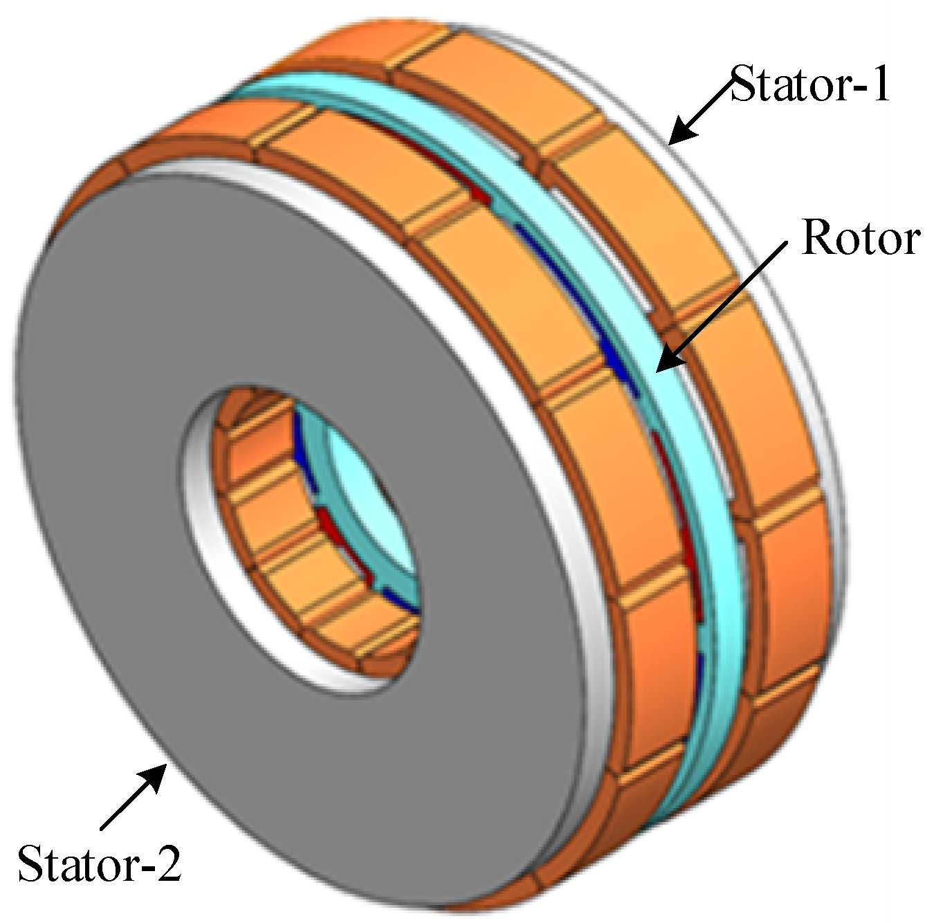
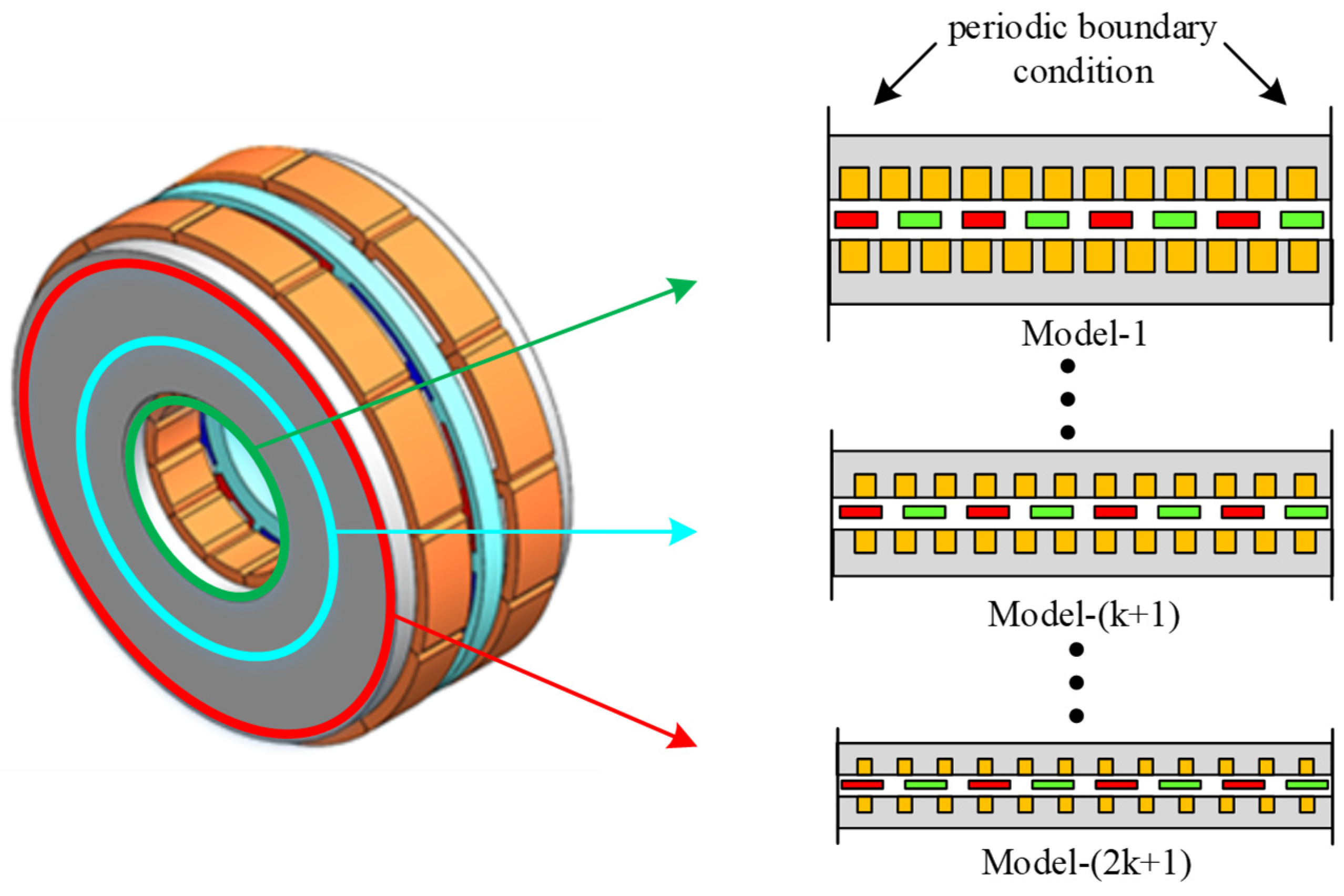
2.1. Three-Dimensional Structure of Axial Flux Permanent Magnet Synchronous Motors

The basic electromagnetic structure of a common axial flux permanent magnet motor is shown in Figure 1 (this article takes a double stator single rotor 12-slot, 10-pole motor as an example), which includes the stator core, winding, rotor permanent magnet, and air gap. The air gap between the stator core and the rotor permanent magnet is the motor’s air gap. As the main magnetic flux of an axial flux motor passes through the motor’s air gap along the axis direction of the motor, it is necessary to use a three-dimensional finite element model to calculate the electromagnetic performance of this type of motor. However, for designers, three-dimensional finite element calculation has extremely strict requirements for computers, requiring the use of high main frequency and large memory scientific research service station computers to achieve calculation. Low-configuration conventional computers usually cannot run calculation programs. To solve this problem, scholars have adopted an equivalent simplified approach to process the axial magnetic flux single machine, reducing its dimensionality from a three-dimensional model to a two-dimensional model, thereby reducing equipment requirements and improving computational efficiency.

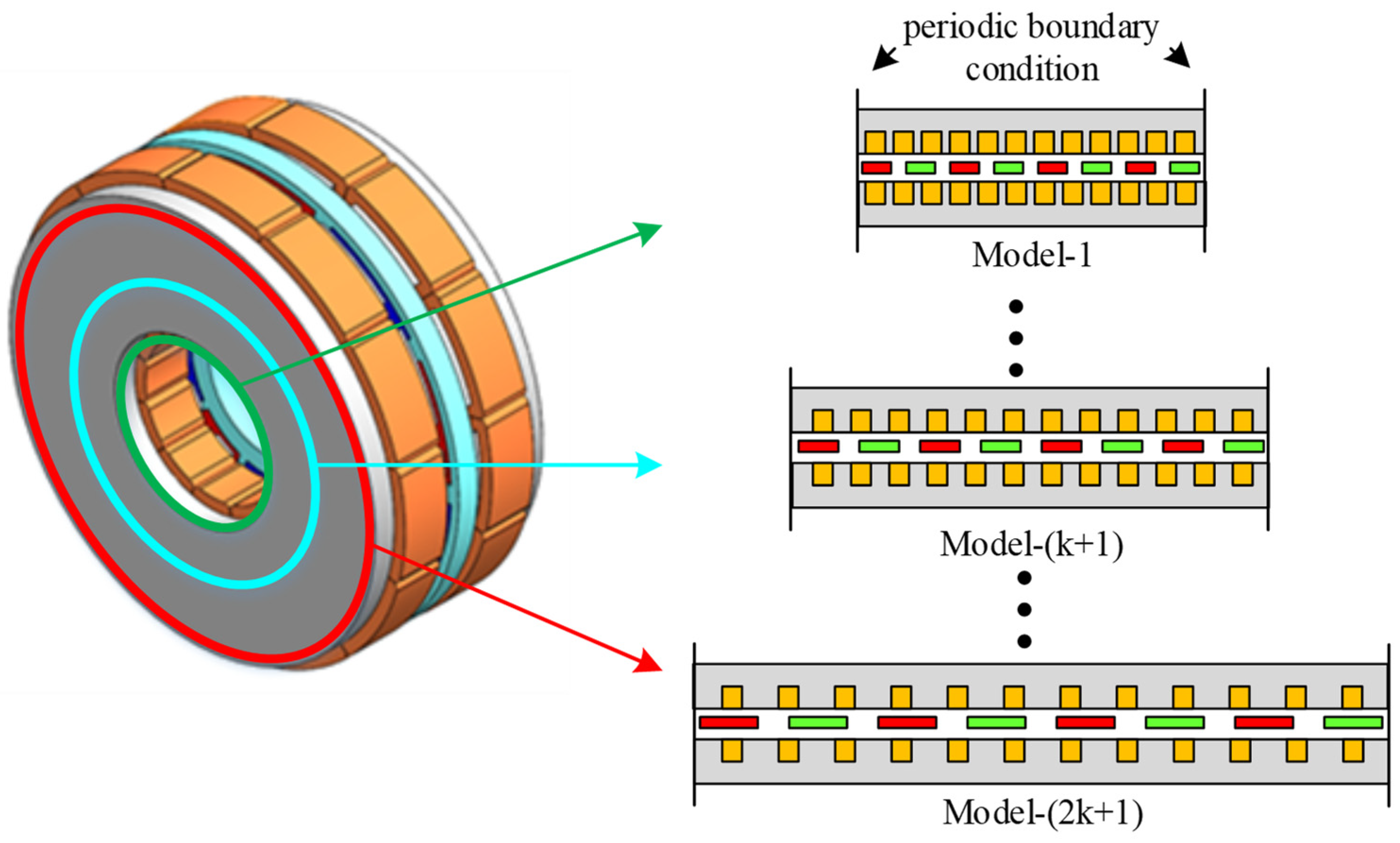
2.2. Existing Equivalent Methods Based on 2D Multi-Layer Linear Permanent Magnet Synchronous Motors

Both the finite element method and analytical method require approximating the three-dimensional axial flux motor model as a two-dimensional motor model. The most common traditional conversion method is to use the linear motor equivalent method to estimate the basic electromagnetic performance of axial flux motors, and the specific process is shown in Figure 2:

• First, divide the expected number of layers, and then calculate the average radius length and thickness of each layer of a thin circular ring;
• Then, calculate the specific parameters of the polar arc coefficient, slot width, tooth width, and slot height of the layer corresponding to its average radius;
• Afterward, an equivalent linear motor model of each layer of a thin circular ring is established in sequence, where the length of the linear motor model is consistent with the average radius circumference, and the tooth slot size of the linear motor is consistent with the previous calculation result;
• Then, for each single-layer model, the materials and boundary conditions need to be set. It should be understood that due to the end magnetic field distortion caused by directly using an equivalent linear motor, calculation errors can be avoided. To avoid this effect, periodic boundary conditions are usually used to set the front and rear end contours of the linear motor. At this time, the linear motor is equivalent to the wireless length, which means there is no end effect;
• Next, calculate the two-dimensional electromagnetic field of the equivalent linear motor in each layer and obtain the force, magnetic linkage, back electromotive force, loss, and other data under no-load and load conditions;
• Finally, perform superposition processing to obtain the final electromagnetic calculation results of the axial flux motor.

The main dimensions of the three-dimensional model of a given axial flux motor are shown in Figure 3:

h_a-3D is the axial height of the stator core on one side, R_i is the inner radius of the axial flux permanent magnet motor, R_o is the outer radius, h_m-3D is the thickness of the permanent magnet, δ is the air gap length, a_p is the pole arc coefficient, h_st-3D is the slot height, w_st-3D is the slot width, N is the number of turns of the concentrated winding, b is the number of teeth of the motor, p is the number of pole pairs of the motor, and Ω is the speed of the motor.

According to the equivalent calculation method shown in Figure 4, the model size conversion relationship between the axial flux motor and the linear motor involved is:

The length of the motion direction of the cth-layer equivalent linear motor is:

$$L_c=2\pi R_{av}^c$$

(1)

$$R_{av}^c=R_i+\frac{R_o-R_i}{n_s}\left(c-\frac{1}{2}\right),c=1,2,\dots k-1,k,k+1,\dots ,n_s$$

where n_s = 2k + 1 is the number of layers.

The stacking thickness of all equivalent linear motors is:

$$l_{linear}=\frac{R_o-R_i}{n_s}$$

(2)

The total height of the iron core of all equivalent linear motors is:

$$h_{linear}=h_{a-3D}$$

(3)

The slot width of all equivalent linear motors is:

$$w_s=w_{st-3D}$$

(4)

The slot height of all equivalent linear motors is:

$$h_s=h_{st-3D}$$

(5)

The winding turns of all equivalent linear motors are:

n = N

(6)

The pole distance of the equivalent linear motor in the cth-layer is:

$${\tau }_c=\frac{L_c}{2p}$$

(7)

The tooth width of the equivalent linear motor in the-layer is:

$$w_t^c=\frac{L_c}{b}-w_s$$

(8)

The distance from the first slot of the cth-layer equivalent linear motor to the boundary is:

$$l_s=\frac{w_t^c}{2}$$

(9)

The thickness of the permanent magnet of the equivalent linear motor in the cth-layer is

$$h_{pm}=h_{m-3D}$$

(10)

The permanent magnet width of the equivalent linear motor in the cth-layer is:

$$l_{pm}={\alpha }_p{\tau }_c$$

(11)

The distance from the first permanent magnet of the cth-layer equivalent linear motor to the boundary is:

$$l_{\mathrm{r}}=\frac{1-{\alpha }_p}{2}{\tau }_c$$

(12)

Based on the model size of the layered equivalent linear synchronous motor mentioned above, after calculating the results, the electromagnetic calculation results of each linear motor can be obtained, while the axial flux motor can be estimated by the following:

The permanent magnet flux linkage of an axial flux motor is:

$${\psi }_{total}={\displaystyle \sum _{c=1}^{n_s}{\psi }_c}={\displaystyle \sum _{c=1}^{n_s}{\displaystyle {\int }_s{B}_{c}ds}}$$

(13)

The no-load back electromotive force of an axial flux motor is:

$$E_{total}=-\frac{\mathrm{d}{\psi }_{total}}{dt}={\displaystyle \sum _{c=1}^{n_s}{E}_c}$$

(14)

The electromagnetic torque of an axial flux motor is:

$$T_{total}={\displaystyle \sum _{c=1}^{n_s}{T}_c}={\displaystyle \sum _{c=1}^{n_s}{F}_c{R}_{av}^c}$$

(15)

The core loss of an axial flux motor is approximately:

$$P_{ironloss}={\displaystyle \sum _{c=1}^{n_s}{P}_{ironloss}^c}$$

(16)

Compared to directly using a three-dimensional finite element model for calculation, the above equivalent method is very fast and has high calculation accuracy. In the author’s opinion, there is still room for further optimization, such as in steps 1–3. It should be understood that due to the frequent use of fractional slot concentrated windings in axial flux motors, the slot space is rectangular in design, meaning that the size of the slot remains unchanged at different radii. This results in a gradual increase in the width of the iron core teeth from the inner radius to the outer radius of the motor. On the other hand, for the convenience of installation and manufacturing, the rotor of axial flux motors is usually designed as a regular sector, meaning that the pole arc coefficient of the motor remains constant at different radii. The structural characteristics of the axial flux motor mentioned above enable a series of linear motor models developed from thin circular rings at different radii to have consistent slot sizes and pole arc coefficients but different total lengths and tooth sizes. In step 3, periodic boundary conditions need to be set separately for each model, which undoubtedly increases the complexity of modeling. To solve the time consumption problem caused by repeated and separate modeling, parameterized models can be used, but boundary conditions beyond the physical size of the model still need to be set separately, and there are also many geometric variables to be parameterized. Therefore, the calculation time of the equivalent model can still be simplified, which is the main work of this article.

3. Improved Equivalent Methods Based on 2D Multi-Layer Linear Permanent Magnet Synchronous Motors

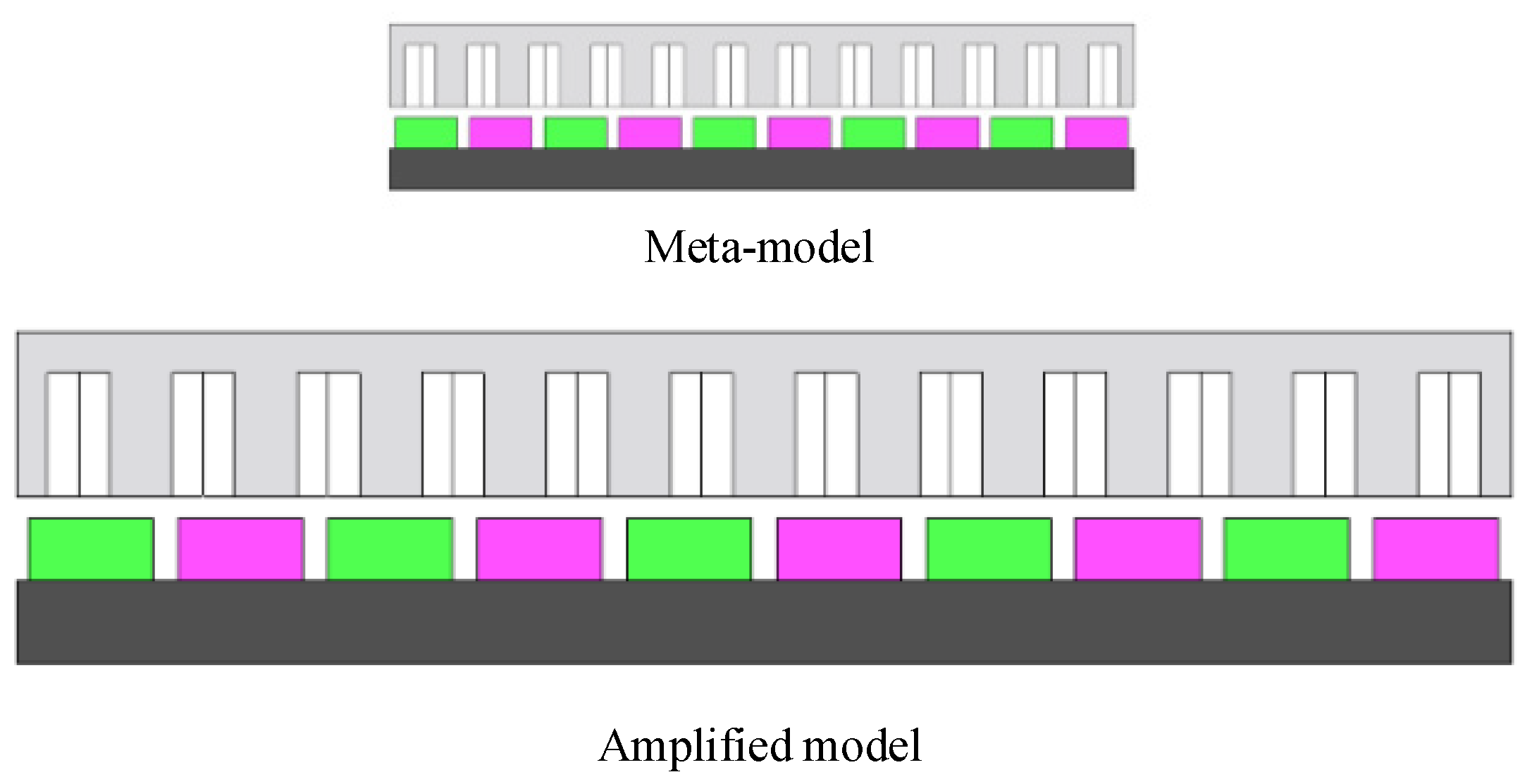
3.1. Analogy Principle of Linear Permanent Magnet Synchronous Motor Model

Before proposing the calculation method in this article, it is necessary to first clarify the corresponding conversion relationship between a series of similar linear motors, that is, how to achieve mutual conversion between the calculation results of two linear motors with different lengths, different tooth widths, the same slot width, different pole distances, and the same pole arc coefficient.

From the knowledge of classical electrical engineering, it can be seen that most of the calculation of electromagnetic performance in a motor is directly related to magnetic density. For example, when calculating force/torque using the Maxwell tension tensor method, it is necessary to know the normal and tangential components of the air gap magnetic flux density:

$$F_t=\frac{L_i}{{\mu }_0}{\displaystyle \int B_n{B}_{t}dl}$$

(17)

When calculating the core loss using the improved Bertotti separation iron loss model, it is necessary to know the magnetic flux density of each part of the core:

$$P_{iron}=G{\displaystyle \sum \left(k_h{B}_m^{\alpha }f+k_c{B}_m^2{f}^2+k_e{B}_m^{1.5}{f}^{1.5}\right)}$$

(18)

Therefore, when applying the analogy effect, attention should be paid to keeping the magnetic flux density of each part in the two models before and after the analogy unchanged. To achieve this goal, taking the 2D linear motor model in Figure 5 as an example, the corresponding relationship between the analog models is as follows:

Their dimensions satisfy the following relationship:

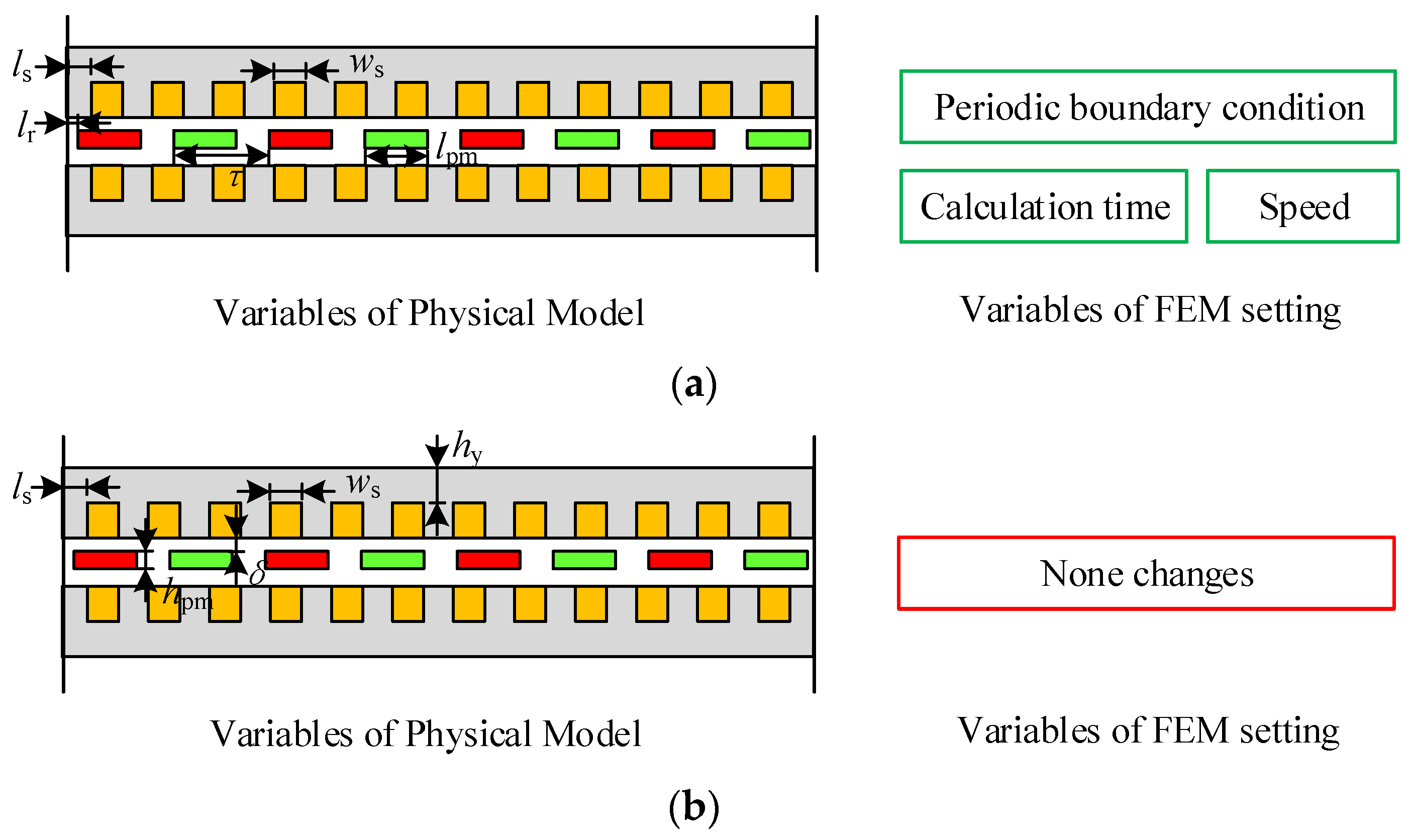
• The values of most major dimensions in the motor are proportionally amplified, including air gap length, permanent magnet thickness, permanent magnet width, pole spacing, tooth width, slot width, yoke height, and current. A small number of dimensional parameters remain unchanged, including material, pole number, slot number, and slot height.
• Set partial current, speed, and other proportional amplification while maintaining consistency in turns, frequency, and calculation steps.

In the above setting mode, calculate the two linear permanent magnet synchronous motor models with dimensions that differ by two times, as shown in Figure 6, and obtain the following calculation results:

It can be seen that under the conditions of maintaining the above dimensions and setting parameters, the distribution characteristics of magnetic density in each part have little difference and are basically consistent.

The relationship between calculation results is shown in Figure 7:

Due to the constant number of turns, the distribution of air gap magnetic density is the same, but the integral area is twice. Therefore, after analogy, the permanent magnet flux is twice as large.

The distribution of air gap density is the same, with an integral area of 2 times, and the values of tangential force are all 2 times the original values.

Due to maintaining frequency consistency, the magnetic flux amplitude is 2 times, the alternating frequency with position changes is 0.5, and the velocity is 2 times, so the back electromotive force frequency remains unchanged, with an amplitude of 2 times.

Due to the consistent pattern of magnetic density changes and the same frequency, but with an increase in volume and weight of square times, after analogy, the iron loss is square times the original value.

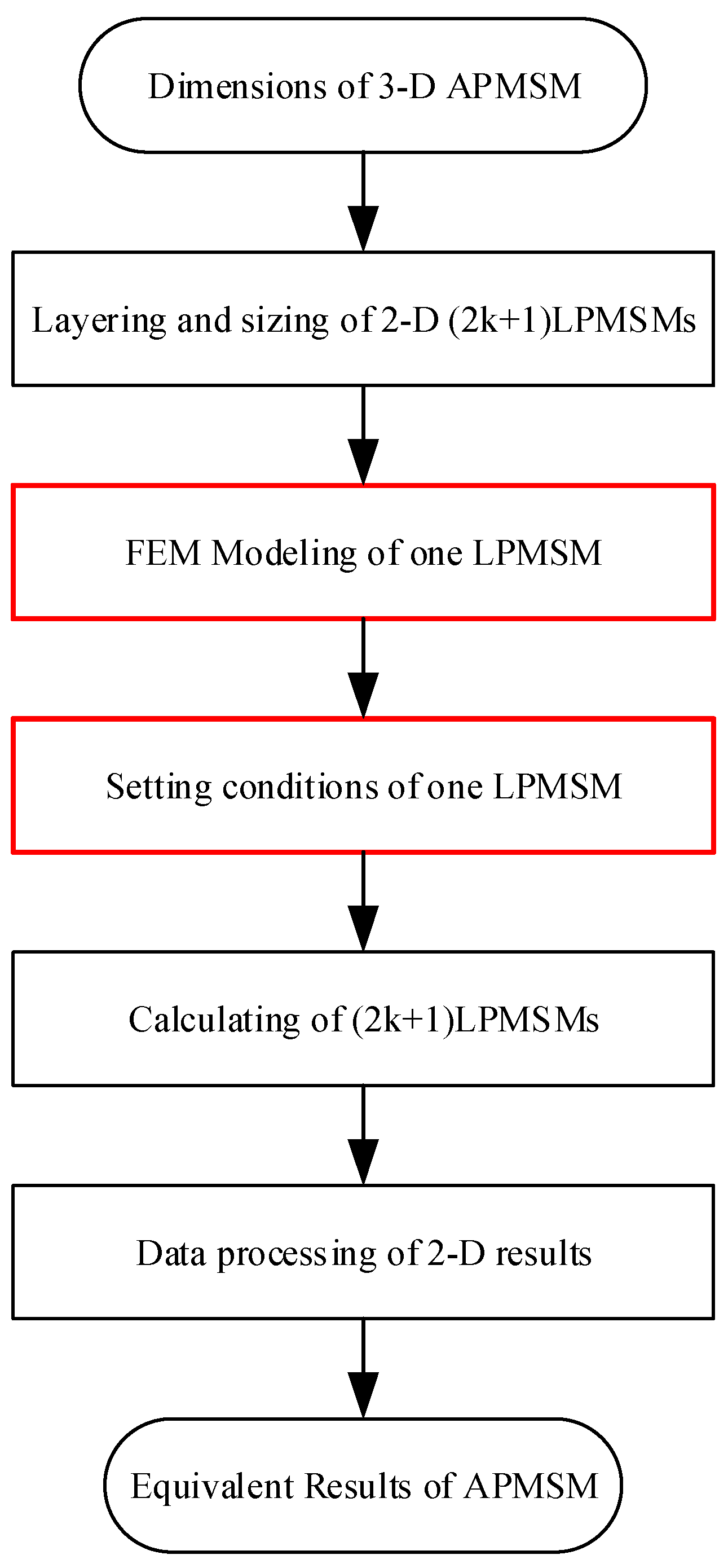
3.2. Improved Equivalent Methods

The equivalent calculation method proposed in this article takes into account the analogy effect between models based on the equivalent method mentioned in the previous section. Thus, by amplifying or reducing in the same proportion, a series of linear motors with different lengths, different tooth widths, the same slot width, the same air gap length, different pole distances, the same permanent magnet thickness, and the same pole arc coefficient are converted into a series of linear motors with the same length, different tooth widths, different slot widths, and the same pole distance. A series of linear motors with different permanent magnet thicknesses, different air gap lengths, and the same pole arc coefficient ensures that the permanent magnet width, motion speed, length of periodic boundary conditions, step size, and calculation time of the equivalent linear motor under different radii are all consistent, eliminating the waste of time on repeatedly setting simulation conditions. The electromagnetic performance of axial flux motors is calculated through only a parameterized linear motor model and data post-processing, further shortening the initial design speed of axial flux motors and improving the speed of subsequent parameter optimization for this type of motor.

As shown in Figure 8, the basic process of proposing an equivalent calculation method in this article is as follows:

Compared with the existing methods in Figure 2, it can be seen from Figure 8 that this article intends to achieve the equivalent calculation of axial flux motor thin ring under different radii by parameterizing a two-dimensional linear motor model through further equivalence at the model level. This can significantly reduce the time spent on two-dimensional motor modeling and further improve the initial calculation speed of the axial flux motor.

The expected calculation process is as follows:

• First, the expected number of layers is divided, and then the average radius length and thickness of each layer of a thin circular ring are calculated;
• Afterward, the specific parameters of the polar arc coefficient, slot width, tooth width, and slot height corresponding to the average radius of the layer are calculated and listed in the parameter table;
• Then, a two-dimensional linear motor model is established based on the parameters of the thin-layer ring in the middle of the motor, which is the overall average radius, and its materials and boundary conditions are set;
• Afterward, five parameters, namely tooth width, slot height, yoke height, permanent magnet thickness, and air gap length, are selected as variables. According to formula 11, the equivalent slot height, tooth width, air gap, and magnetic steel thickness at different radii are calculated sequentially, and they are set in the linear motor model in the previous step;
• Next, the two-dimensional electromagnetic field is calculated under different parameter conditions, and the force, magnetic linkage, back electromotive force, loss, and other data under no-load and load conditions are obtained;
• Finally, the electromagnetic calculation results of the axial flux motor are obtained by superposition processing.

Based on the above ideas, the new model conversion calculation formula should be introduced clearly. Compared with the original method, the size conversion formula has changed, and a scaling factor is introduced on the basis of the formula:

$$K_{ratio}^c=\frac{L_c}{\pi \left(R_i+R_o\right)}=\frac{2R_{av}^c}{R_i+R_o}$$

(19)

Correspondingly, each size changes separately.

The motion direction and length of all equivalent linear motors are equal, all of which are:

$$L_c=\pi \left(R_i+R_o\right)$$

(20)

The stacking thickness of all equivalent linear motors is:

$$l_{linear}=\frac{R_o-R_i}{n_s}$$

(21)

The total height of the iron core of the cth-layer equivalent linear motor is:

$$h_{linear}^c=h_{a-3D}/K_{ratio}^c$$

(22)

The slot width of the cth-layer equivalent linear motor is:

$$w_s^c=w_{st-3D}/K_{ratio}^c$$

(23)

The slot height of the equivalent linear motor in the cth-layer is:

$$h_s^c=h_{st-3D}/K_{ratio}^c$$

(24)

The winding turns of all equivalent linear motors are:

n = N

(25)

The pole distance of all equivalent linear motors is:

$${\tau }_c=\frac{\pi \left(R_i+R_o\right)}{2p}$$

(26)

The tooth width of the equivalent linear motor in cth-layer is:

$$w_t^c=\frac{L_c}{b}-w_s^c$$

(27)

The distance from the first slot of the cth-layer equivalent linear motor to the boundary is:

$$l_s=\frac{w_t^c}{2}$$

(28)

The thickness of the permanent magnet of the equivalent linear motor in cth-layer is:

$$h_{pm}^c=h_{m-3D}/K_{ratio}^c$$

(29)

The air gap length of the cth-layer equivalent linear motor is:

$${\delta }_c={\delta }_{3D}/K_{ratio}^c$$

(30)

The permanent magnet width of all equivalent linear motors is:

$$l_{pm}={\alpha }_p{\tau }_c=\frac{{\alpha }_p\pi \left(R_i+R_o\right)}{2p}$$

(31)

The distance from the first permanent magnet of all equivalent linear motors to the boundary is:

$$l_{\mathrm{r}}=\frac{1-{\alpha }_p}{2}{\tau }_c=\frac{\pi \left(R_i+R_o\right)\left(1-{\alpha }_p\right)}{4p}$$

(32)

After the above transformation, the three-dimensional axial flux motor is transformed into a series of two-dimensional linear motors, as shown in Figure 9. The permanent magnet width, motion speed, length of periodic boundary conditions, step size, and calculation time of all linear motors are consistent. After calculating the results, the electromagnetic calculation results of each linear motor can be obtained. By combining the principle of analogy, the axial flux motor can be estimated through the following post-processing steps.

The permanent magnet flux linkage of an axial flux motor is:

$${\psi }_{total}={\displaystyle \sum _{c=1}^{n_s}{\psi }_c{K}_{ratio}^c}={\displaystyle \sum _{c=1}^{n_s}{K}_{ratio}^c{\displaystyle {\int }_s{B}_{c}ds}}$$

(33)

The no-load back electromotive force of an axial flux motor is:

$$E_{total}=-\frac{\mathrm{d}{\psi }_{total}}{dt}={\displaystyle \sum _{c=1}^{n_s}{K}_{ratio}^c{E}_c}$$

(34)

The electromagnetic torque of an axial flux motor is:

$$T_{total}={\displaystyle \sum _{c=1}^{n_s}{K}_{ratio}^c{T}_c}={\displaystyle \sum _{c=1}^{n_s}{K}_{ratio}^c{F}_c{R}_{av}^c}$$

(35)

The core loss of an axial flux motor is approximately:

$$P_{ironloss}={\displaystyle \sum _{c=1}^{n_s}{\left(K_{ratio}^c\right)}^2{P}_{ironloss}^c}$$

(36)

The comparison between the model size variables and model setting variables included in the equivalence of the two methods is shown in Figure 10. For traditional equivalent methods, although the electrical angular velocity and frequency of each equivalent linear motor are consistent, the motion of the equivalent linear motor model at different radii is different, and the simulation conditions that need to be set in the corresponding solution are different, such as the setting of speed and periodic boundary conditions, the step size of the solver, and the calculated steps/total calculation time. Therefore, the original method requires N independent linear permanent magnet synchronous motor models or establishing a linear motor model with five parameterized variables and setting independent conditions with three variables for each motor model. By comparison, it can be seen that the equivalent method proposed in this article only requires the establishment of one linear permanent magnet synchronous motor model with five parameterized variables. The settings and solving conditions of all Ns models are completely consistent, and there is no need for independent modification. It can be seen that the calculation method proposed in this article can achieve a fast estimation of axial flux motors with fewer computational resources.

4. Validation of Proposed Method

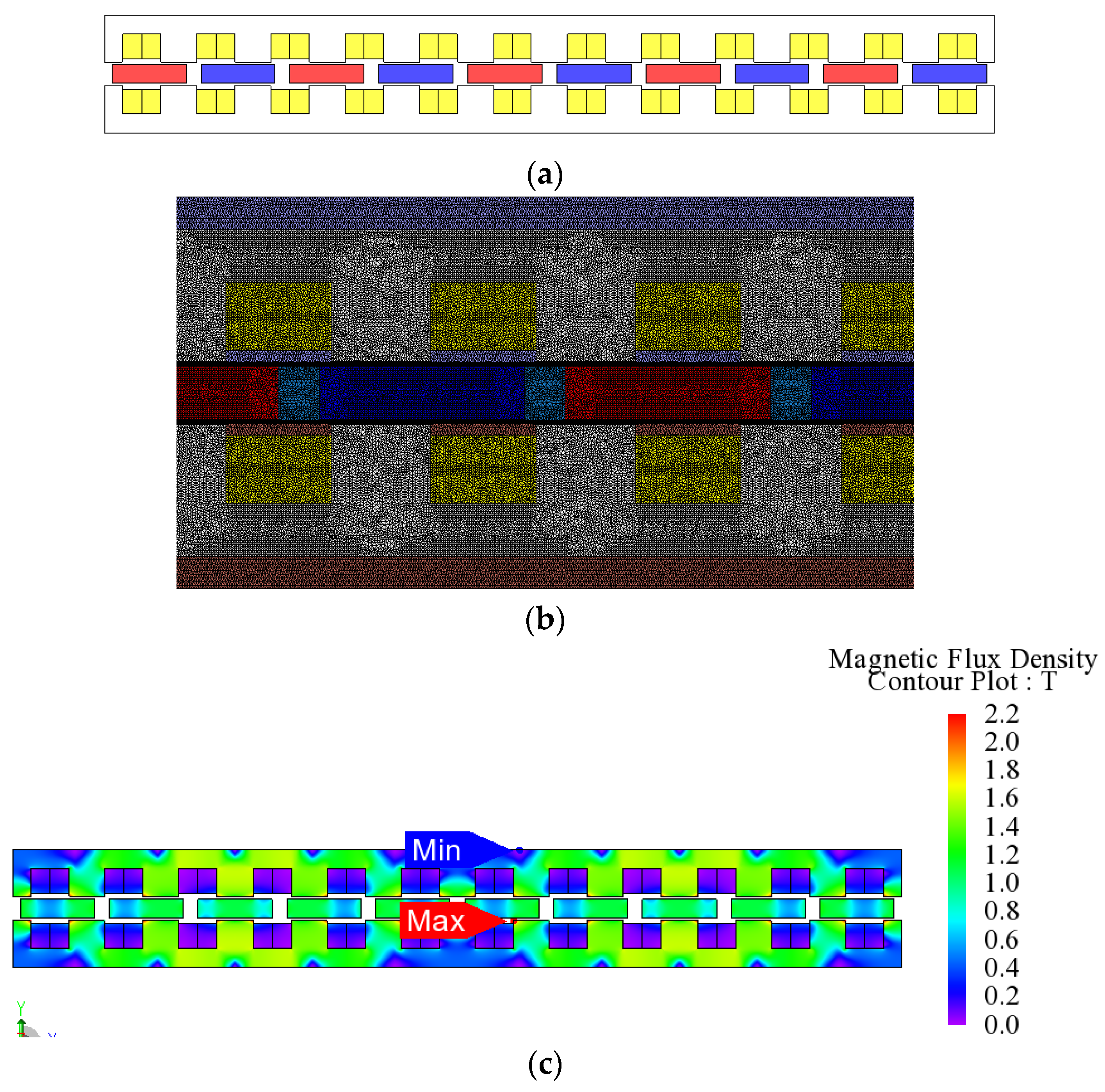
4.1. Three-Dimensional Model and Proposed Two-Dimensional Model

To verify the effectiveness of the aforementioned methods, the electromagnetic performance of an axial flux permanent magnet synchronous motor with a 10-pole, 12-slot double-sided stator and a single rotor in series magnetic circuit form is calculated using the three-dimensional finite element method and the two-dimensional equivalent finite element method proposed in this paper. The size parameters of the corresponding model are shown in

Table 1. Size parameters of axial flux permanent magnet synchronous motor.

Size Parameter	Parameter Value
Inner radius of stator core (mm)	50
Outer radius of stator core (mm)	100
Permanent magnet thickness (mm)	10
Air gap length (mm)	1
Width of stator slot (mm)	20
Stator slot depth (mm)	15
Single stator axial length (mm)	25
Permanent magnet material	NdFeB42
Number of turns (turns)	76
Rated speed (r/min)	600
Polar arc coefficient	0.83
Number of poles	10
Number of slots	12
Inner radius of permanent magnet (mm)	50

.

Here, taking the nine-segment division method as an example, a two-dimensional equivalent linear motor model of the motor is established, where the average radius and scaling coefficient corresponding to each layer are shown in

Table 2. Average radius and scaling coefficient.

Layered Serial Number	Average Radius	Scaling Coefficient
1st	52.77778	0.7037
2nd	58.33333	0.77778
3rd	63.88889	0.85185
4th	69.44444	0.92593
5th	75	1
6th	80.55556	1.07407
7th	86.11111	1.14815
8th	91.66667	1.22222
9th	97.22222	1.2963

.

According to the above dimensions and materials, the three-dimensional model and two-dimensional model of the axial flux permanent magnet synchronous motor are, respectively, established. Because the motor has symmetry, in order to reduce the time of three-dimensional calculation, the complete motor model is simplified into a quarter model according to the symmetry relationship and is halved along the axial direction and tangential direction of the motor. The simplified 3D motor model and meshing situation are shown in Figure 11, with a mesh element number of 1,366,668 and a node number of 307,790, respectively. According to the two-dimensional equivalent method described in the previous chapter, a two-dimensional linear motor equivalent model of the motor is established, as shown in Figure 12. Due to the fast calculation speed of two-dimensional, in order to simplify it symmetrically, if it is necessary to further improve the calculation speed, the model can be treated similarly with reference to three-dimensional symmetry. The mesh element number and node number of the linear motor model in the middle layer shown in Figure 12 are 282,786 and 149,043, respectively. Here, the maximum edge length for both 3D and 2D sections is maintained to be 0.5 mm.

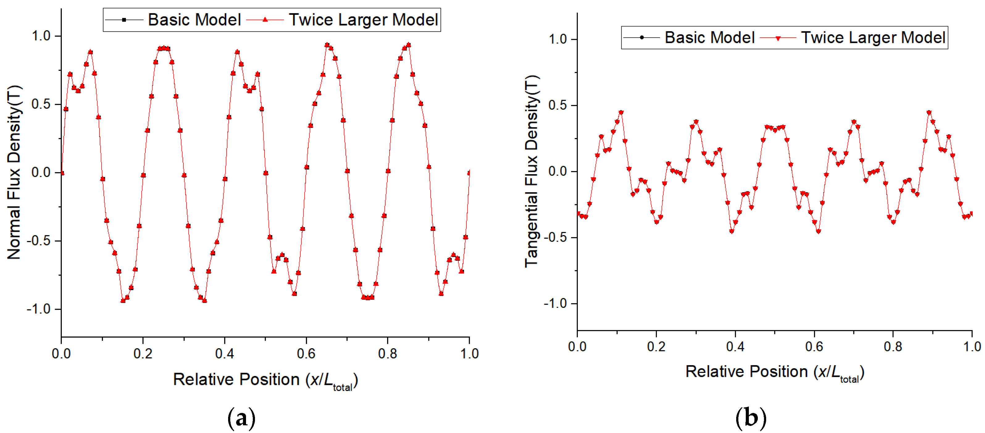
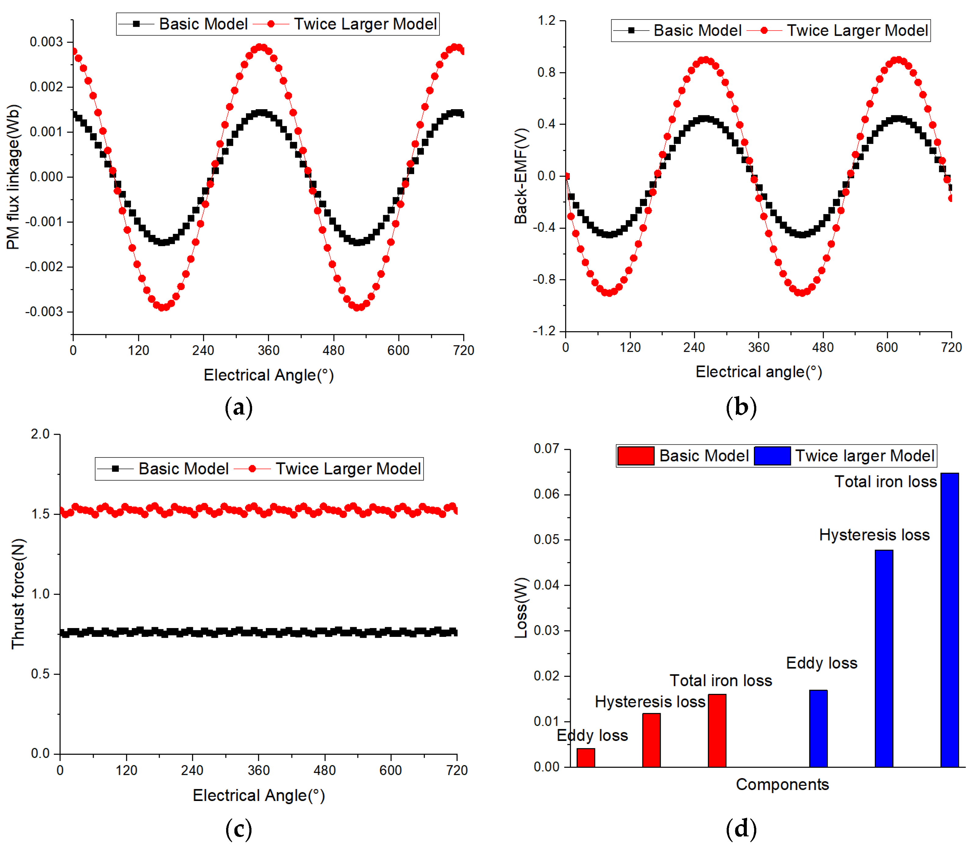
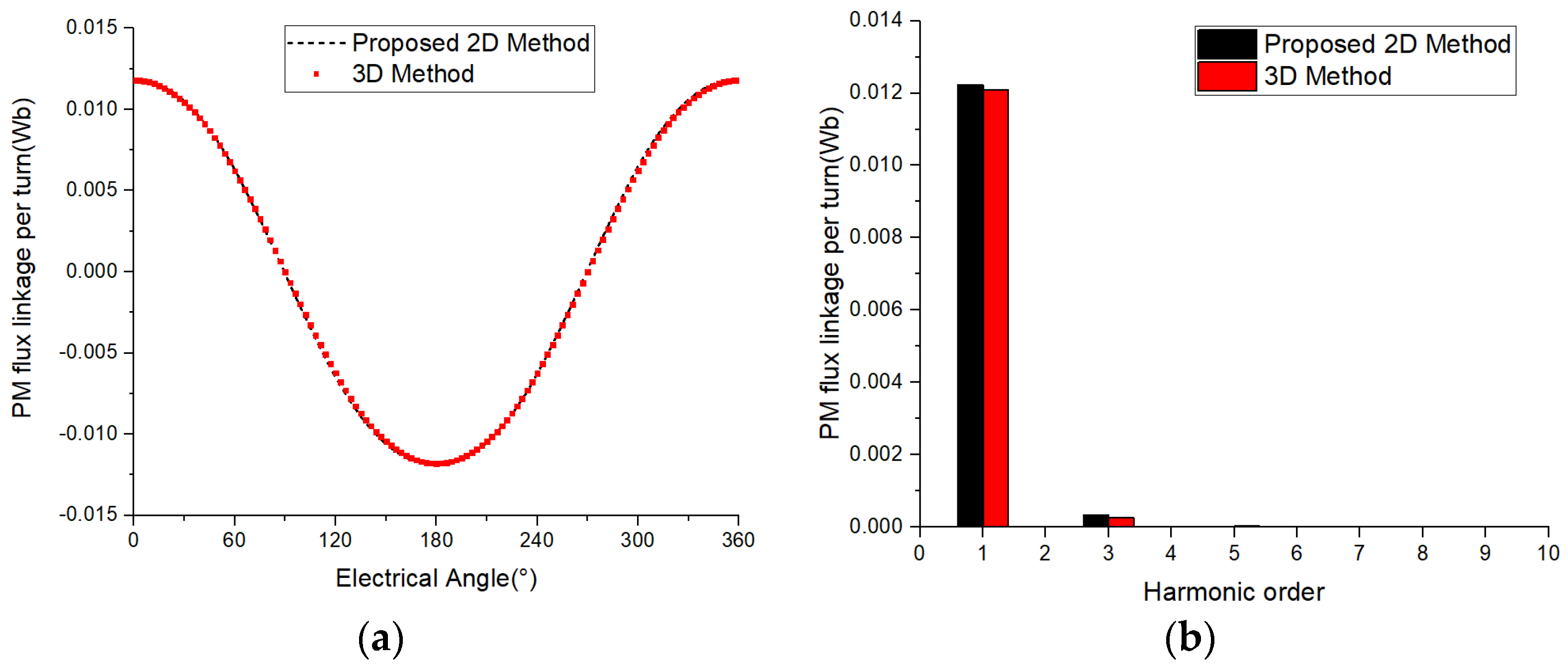
4.2. Comparison of Permanent Magnetic Flux Linkage

When no current is applied to the winding, the magnetic flux of the cross-linked winding is generated by permanent magnet excitation. For the design and control of permanent magnet synchronous motors, the value of the permanent magnet magnetic flux is very important. The waveform of the permanent magnet flux calculated by the 2D and 3D methods is shown in Figure 13a, which roughly appears to be almost identical. Further Fourier decomposition was performed to obtain the harmonic distribution of the two methods, as shown in Figure 13b. From the results, it can be seen that the fundamental amplitude of the permanent magnet flux is 0.01223 Wb and 0.01208 Wb, respectively, with a numerical error of only 1.23% between the two. The maximum harmonic component of the permanent magnet flux in both methods is the third harmonic, with amplitudes of 3.29801 × 10⁻⁴ and 2.54954 × 10⁻⁴ Wb, respectively. It can be seen that the third harmonic component obtained by the 2D equivalent method is relatively large, but it is still very small for the fundamental amplitude.

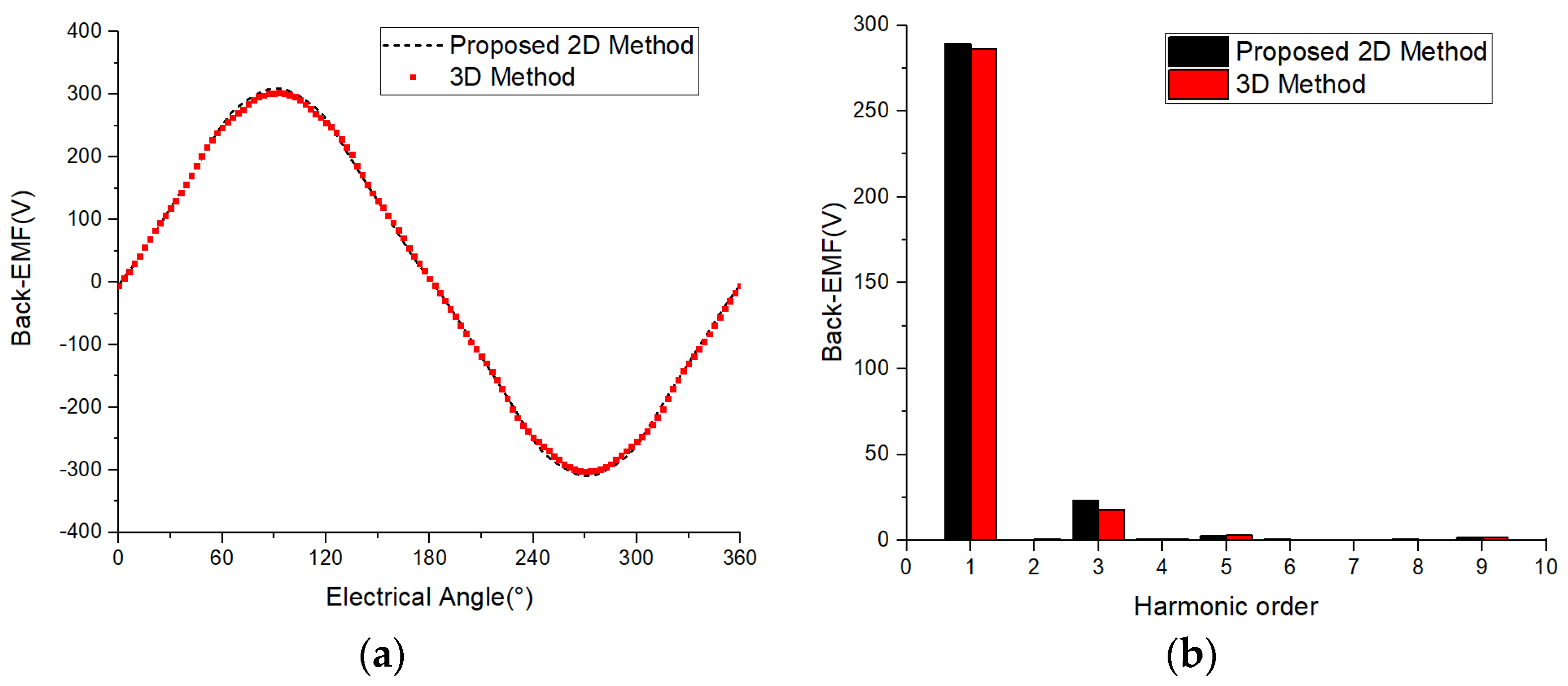
4.3. Comparison of No-Load Back Electromotive Force

The no-load back electromotive force is the differential of the permanent magnet flux with respect to time. The waveform of the permanent magnet flux calculated by 2D and 3D methods is shown in Figure 14a, which roughly appears to be almost completely coincident, and the shape of the sine is relatively high, with only slight deviations at the peak and valley values. Further Fourier decomposition was performed to obtain the harmonic distribution of the two methods, as shown in Figure 14b. From the results, it can be seen that the fundamental amplitudes of the no-load back electromotive force are 289.07568 V and 286.13794 V, respectively, with a numerical error of only 1.01% between the two. The maximum harmonic component of the no-load back EMF in both methods is the third harmonic, with amplitudes of 23.35874 V and 17.99104 V, respectively. It can be seen that the third harmonic component obtained by the 2D equivalent method is relatively large, but it is still very small for the fundamental amplitude. The THD values of the two are 8.15% and 7.05%, respectively, indicating a small difference in the sine degree of the motor’s back electromotive force.

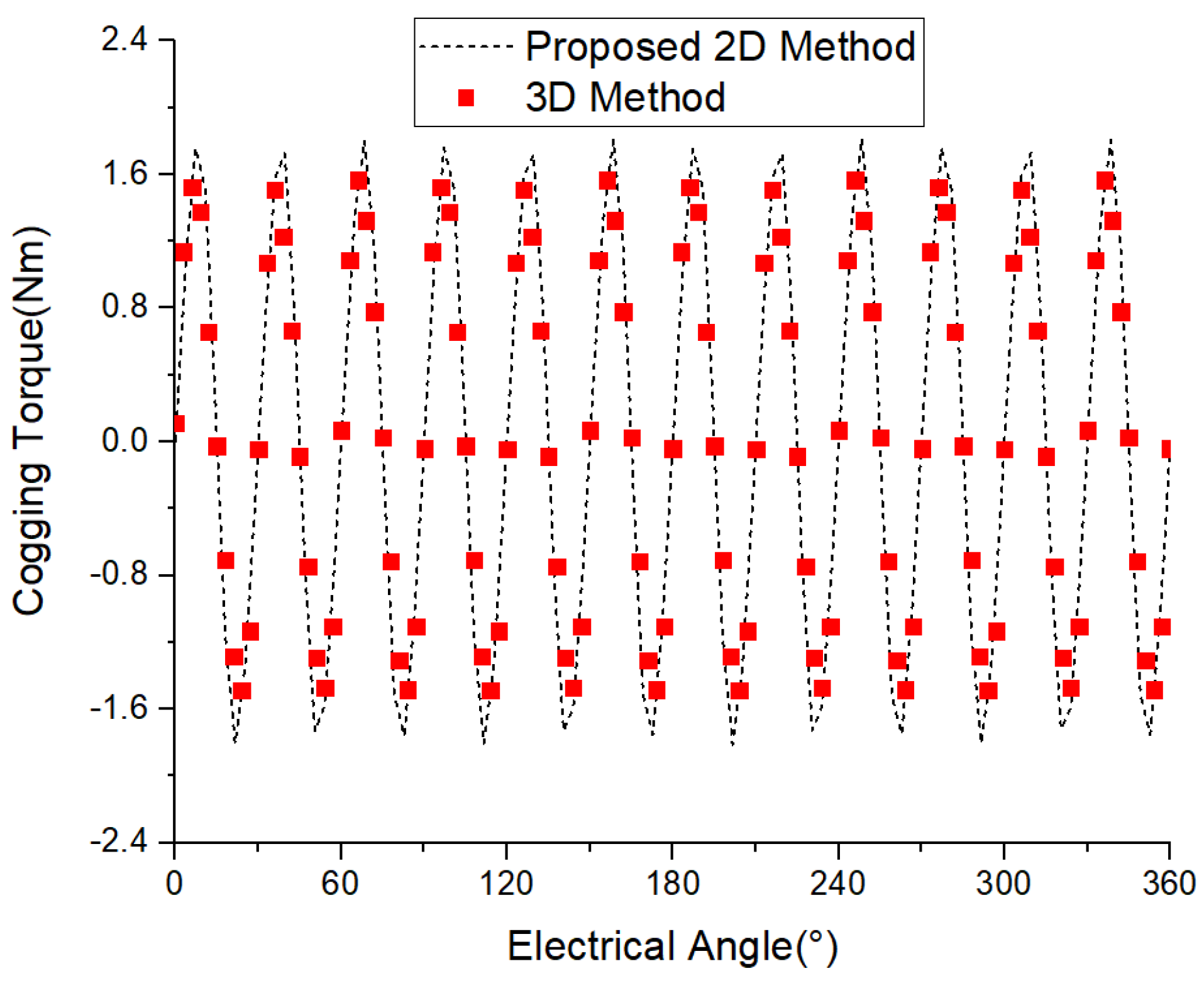
4.4. Comparison of Cogging Torque

The positioning torque is generated by the interaction between the permanent magnet magnetomotive force and the changes in air gap permeability caused by slotting and is also one of the sources of torque pulsation and noise in the practical application of electric motors. The waveform of the permanent magnet flux chain calculated by the 2D and 3D methods is shown in Figure 15, which roughly appears to be almost completely coincident with each other, presenting a form of 12th harmonic within an electrical cycle. The positioning torque amplitudes obtained by the two methods are 1.71 Nm and 1.59 Nm, respectively, with a numerical error of only 7.01% between the two. It can be seen that the value of the positioning torque obtained by the 2D equivalent method is relatively large, but the error meets the engineering requirements in the preliminary design and optimization.

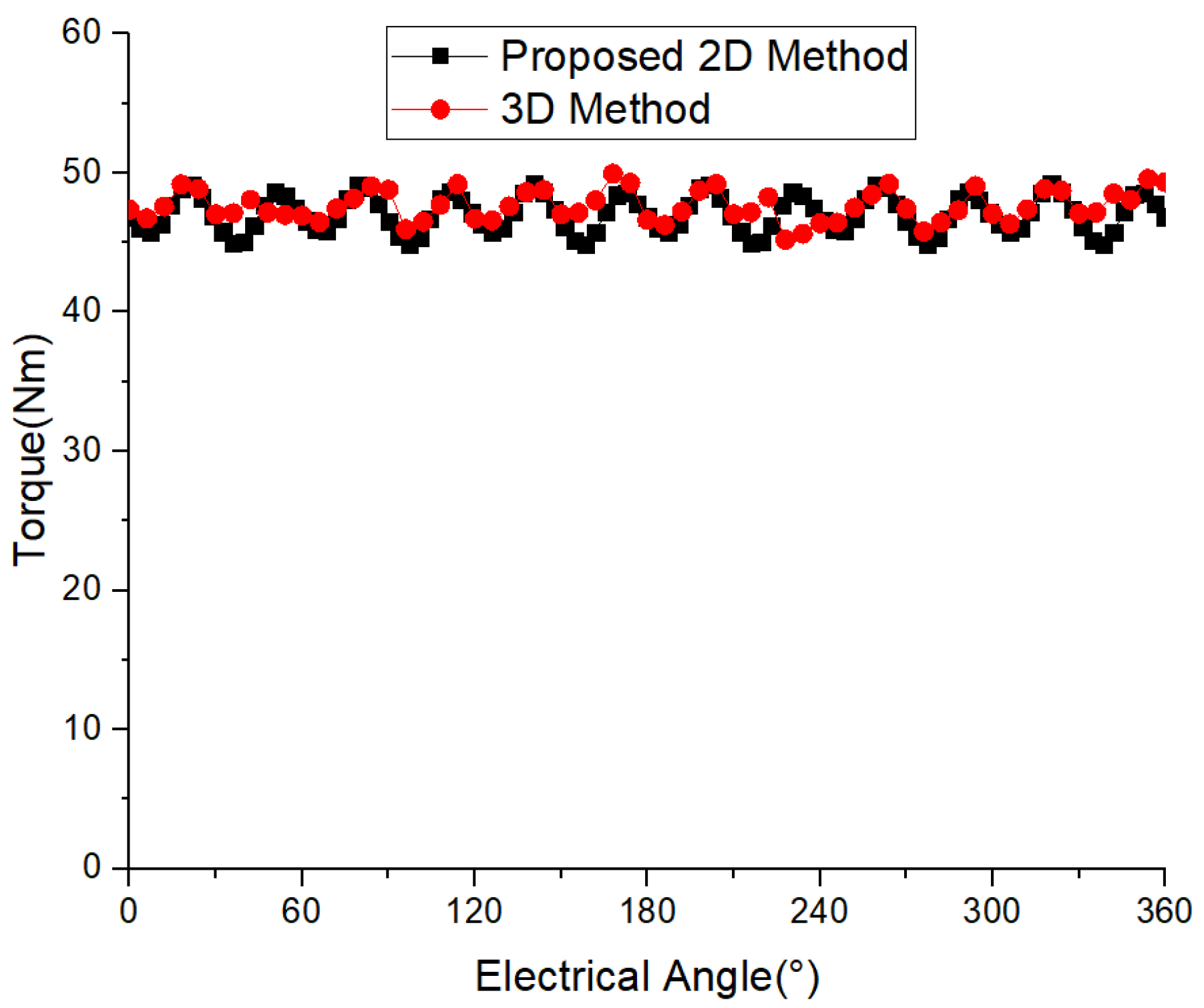
4.5. Comparison of Electromagnetic Torque

Axial flux motors are used to drive loads for various rotational movements, so electromagnetic torque must be calculated in engineering design. The waveform of the electromagnetic torque calculated by the 2D and 3D methods is shown in Figure 16, which roughly appears to be almost completely coincident, exhibiting a 12th harmonic within an electrical cycle. The electromagnetic torque amplitudes obtained by the two methods are 47.85 Nm and 47.63 Nm, respectively, with a numerical error of only 1.2% between the two. For torque fluctuation, the fluctuation value calculated by 2D is 4.85 Nm, with a fluctuation ratio of 9.24%, and the fluctuation value calculated by 3D is 4.72 Nm, with a fluctuation ratio of 9.90%. The calculation results of the two methods are very close, and the error meets the engineering requirements in preliminary design and optimization.

4.6. Comparison of Iron Loss

The copper loss of the winding during the preliminary design process can be directly obtained by multiplying the square of the current by the resistance. For both the 2D and 3D methods, the copper loss of the motor is a theoretical estimate and is completely equal. Therefore, the core loss on the stator side is the main comparison object for verifying the feasibility of the model. The iron core loss is an essential component in the loss evaluation of axial flux permanent magnet synchronous motors. The values of iron core loss calculated by 2D and 3D methods are 31.18793 W and 31.69523 W, respectively, with a deviation of only 1.60% between the two methods. The calculation results of the two methods are very close.

Unfortunately, based on the calculation principle of the eddy current losses in the permanent magnet, it is currently not suitable to simulate and calculate eddy current losses in permanent magnets with fan-shaped shapes using a two-dimensional linear motor equivalent model, which is one of our future research goals.

4.7. Calculation Time

In the analysis of no load and load mentioned above, the simulation steps for one electrical cycle are set to 101 steps, and the same hardware of the computer is used. The calculation time for a single 3D model under one operating condition is about 100 h. Under the same conditions, the calculation time for a single 2D model under one working condition is about 20 min. The results are calculated sequentially at each layer and processed. The overall time consumption for one single working condition using the proposed two-dimensional multi-layer linear permanent magnet synchronous motor is about 20 × 9 min = 3 h. That is, under the premise that the calculation results are very close and the error meets the engineering requirements in the preliminary design and optimization, the time consumption of the method proposed in this article is only 3% of the 3D method. It should be noted that the 3D model is a quarter model, and the 2D model has not been simplified. If the same half model or quarter model is used, its calculation speed will be further improved.

In addition, to demonstrate the comparison between the proposed method in this article and the traditional two-dimensional method mentioned in Section 2.2, detailed calculation time data are listed in

Table 3. Comparison of calculation times for three methods.

Time-Consuming	Unit	3D FEM	Existed 2D FEM	Proposed 2D FEM
Geometric modeling	min	15	5 × 9 = 45	5
Simulation settings	min	3	3 × 9 = 45	3
Solution time	min	6000	20 × 9 = 180	20 × 9 = 180
Result processing time	min	3	10	10
Total time	min	6021	280	198

. To demonstrate differences, there are some subjective variables in the comparison time (such as the time when the model was established and the time when the parameters were set). Among them, the modeling of the 3D model is relatively complex, taking 15 min, but only needs to be modeled once, and for fixed motor sizes and parameters, there is no need to select a parameterized model. The simulation setup process of the 3D model also only needs to be executed once, and all are objective calculation times.

For the traditional method shown in Figure 2, although establishing a single model only takes 5 min, modeling a 2D model requires nine times longer. In addition, due to the different simulation conditions in each new 2D model with changed parameters, it is necessary to set the simulation conditions once, including the simulation step size, speed, and position of periodic boundary conditions. This process needs to be repeated nine times, taking 45 min. In addition, the solution time is about 180 min, and the result processing time is about 10 min, totaling 280 min.

For the improved method proposed in this article, although there is no essential difference in solving time compared to traditional methods, the 2D model of this method only needs to be modeled once. By selecting five geometric parameters to achieve each layered overlay model, the simulation conditions of all models are consistent. Therefore, the positions of rotational speed, step size, and periodic boundary conditions only need to be set once, and the total time required for the result processing process is only 188 min. Based on the necessary objective calculation time, it can be seen that the timeliness and convenience of the proposed method in this article are obvious.

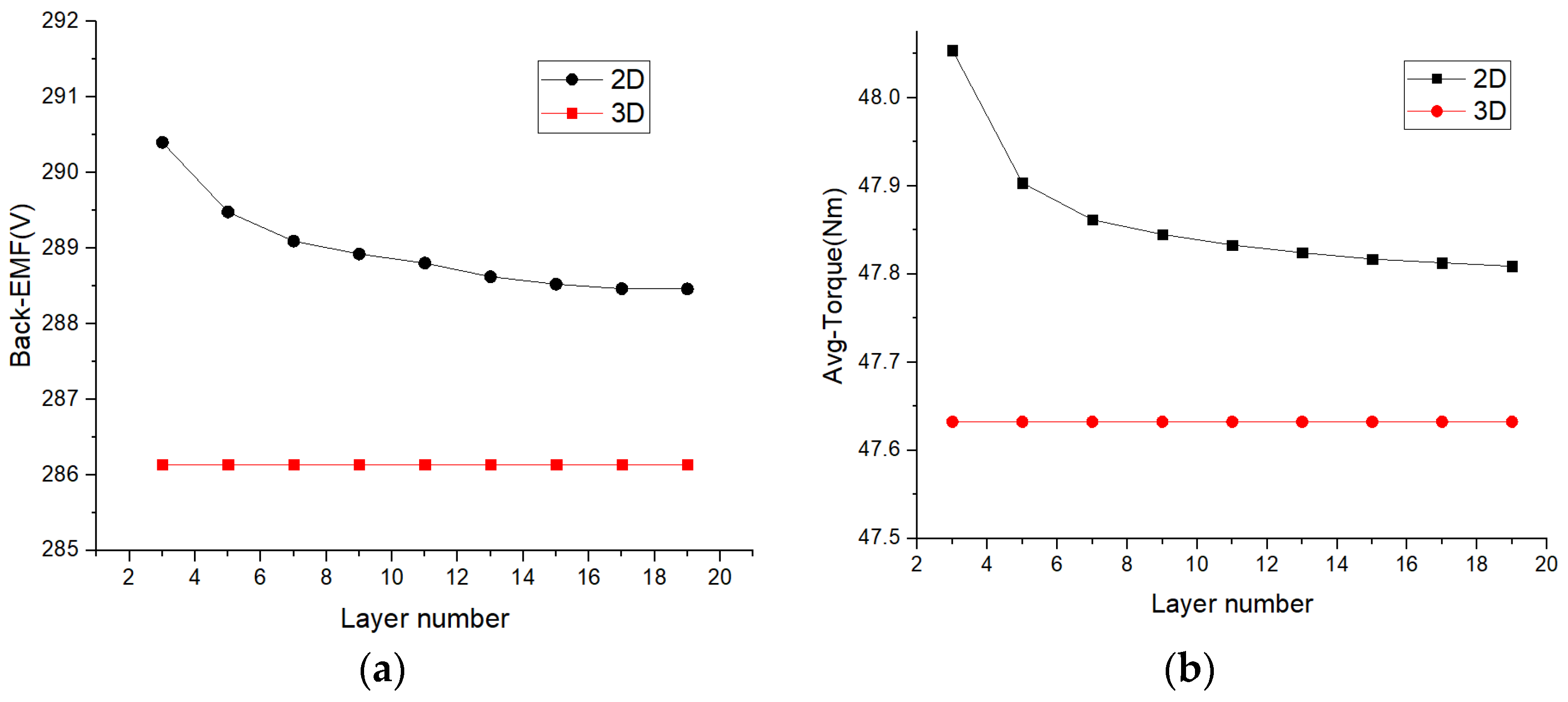
4.8. Impact of the Number of Layers on the Results

In order to supplement the analysis of the impact of the number of layers on the proposed method, a calculation model for dividing the method from 3 layers to 19 layers is established. The average radius under different dividing methods is shown in

Table 4. Number of layers and corresponding equivalent radii of each layer.

	3-Layer	5-Layer	7-Layer	9-Layer	11-Layer	13-Layer	15-Layer	17-Layer	19-Layer
1st	58.33333	55	53.57143	52.77778	52.27273	51.92308	51.66667	51.47059	51.31579
2nd	75	65	60.71429	58.33333	56.81818	55.76923	55	54.41176	53.94737
3rd	91.66667	75	67.85714	63.88889	61.36364	59.61538	58.33333	57.35294	56.57895
4th		85	75	69.44444	65.90909	63.46154	61.66667	60.29412	59.21053
5th		95	82.14286	75	70.45455	67.30769	65	63.23529	61.84211
6th			89.28571	80.55556	75	71.15385	68.33333	66.17647	64.47368
7th			96.42857	86.11111	79.54545	75	71.66667	69.11765	67.10526
8th				91.66667	84.09091	78.84615	75	72.05882	69.73684
9th				97.22222	88.63636	82.69231	78.33333	75	72.36842
10th					93.18182	86.53846	81.66667	77.94118	75
11th					97.72727	90.38462	85	80.88235	77.63158
12th						94.23077	88.33333	83.82353	80.26316
13th						98.07692	91.66667	86.76471	82.89474
14th							95	89.70588	85.52632
15th							98.33333	92.64706	88.15789
16th								95.58824	90.78947
17th								98.52941	93.42105
18th									96.05263
19th									98.68421

, and the results are organized and analyzed using the aforementioned method. Taking the amplitude of the fundamental wave of the back electromotive force and the average electromagnetic torque as examples, the results are shown in Figure 17. It can be seen that as the number of layers increases, the calculation results of the 2D method are closer to those of the 3D method; that is, the more layers there are, the more accurate the calculation results are. In the current example size, when the number of layers exceeds nine, the impact of the number of layers is not significant. Therefore, in the subsequent practical application process, it is necessary to select the appropriate number of layers based on the actual size and accuracy requirements of the calculation model. It should be noted that due to the inability of the 2D method to consider the impact of end leakage flux on axial flux permanent magnet synchronous motors, the calculation errors caused by these factors cannot be solved by increasing the number of layers. One of our future key tasks is to quickly and accurately consider the impact of magnetic flux leakage at the end of this three-dimensional model.

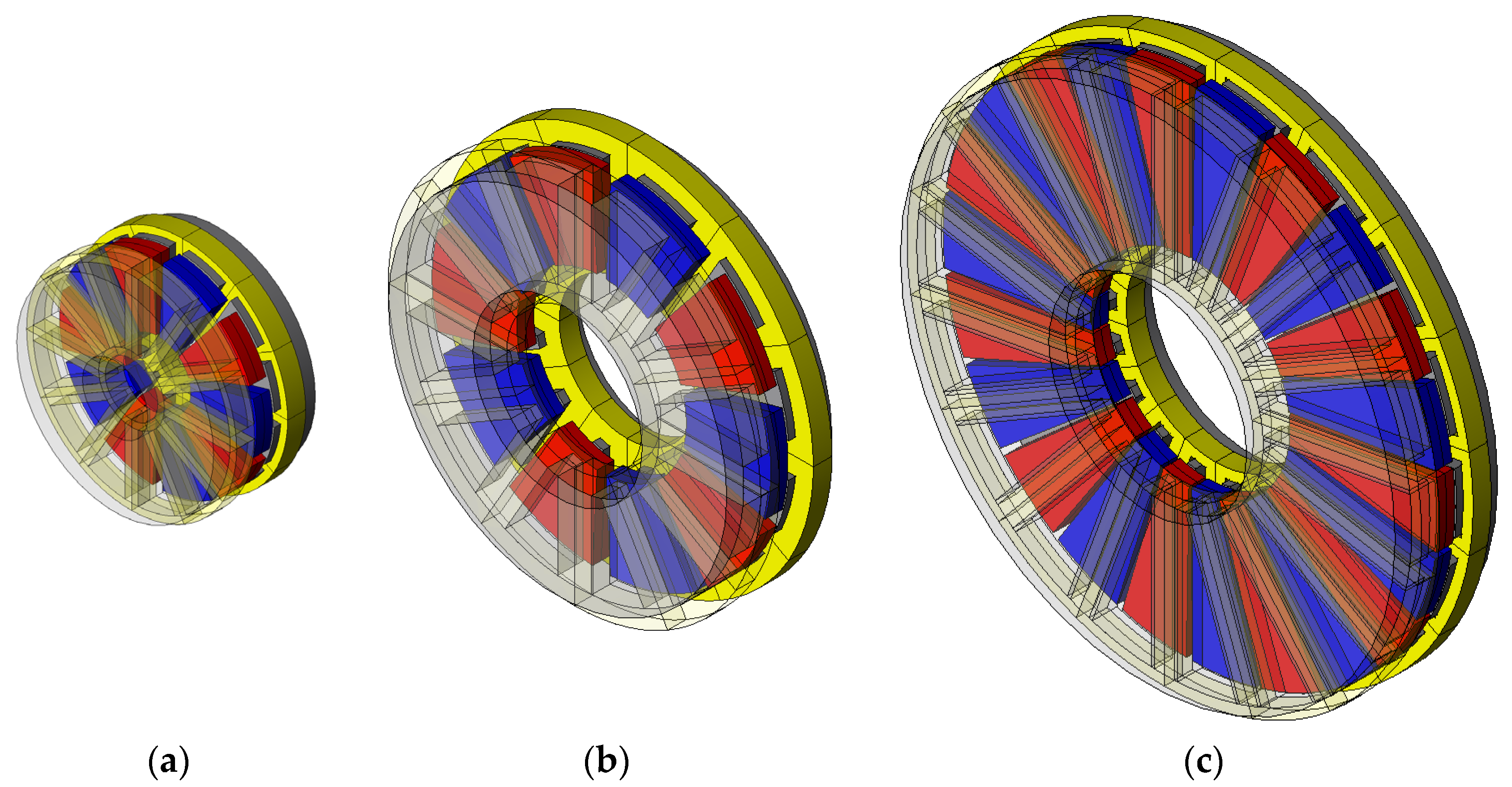
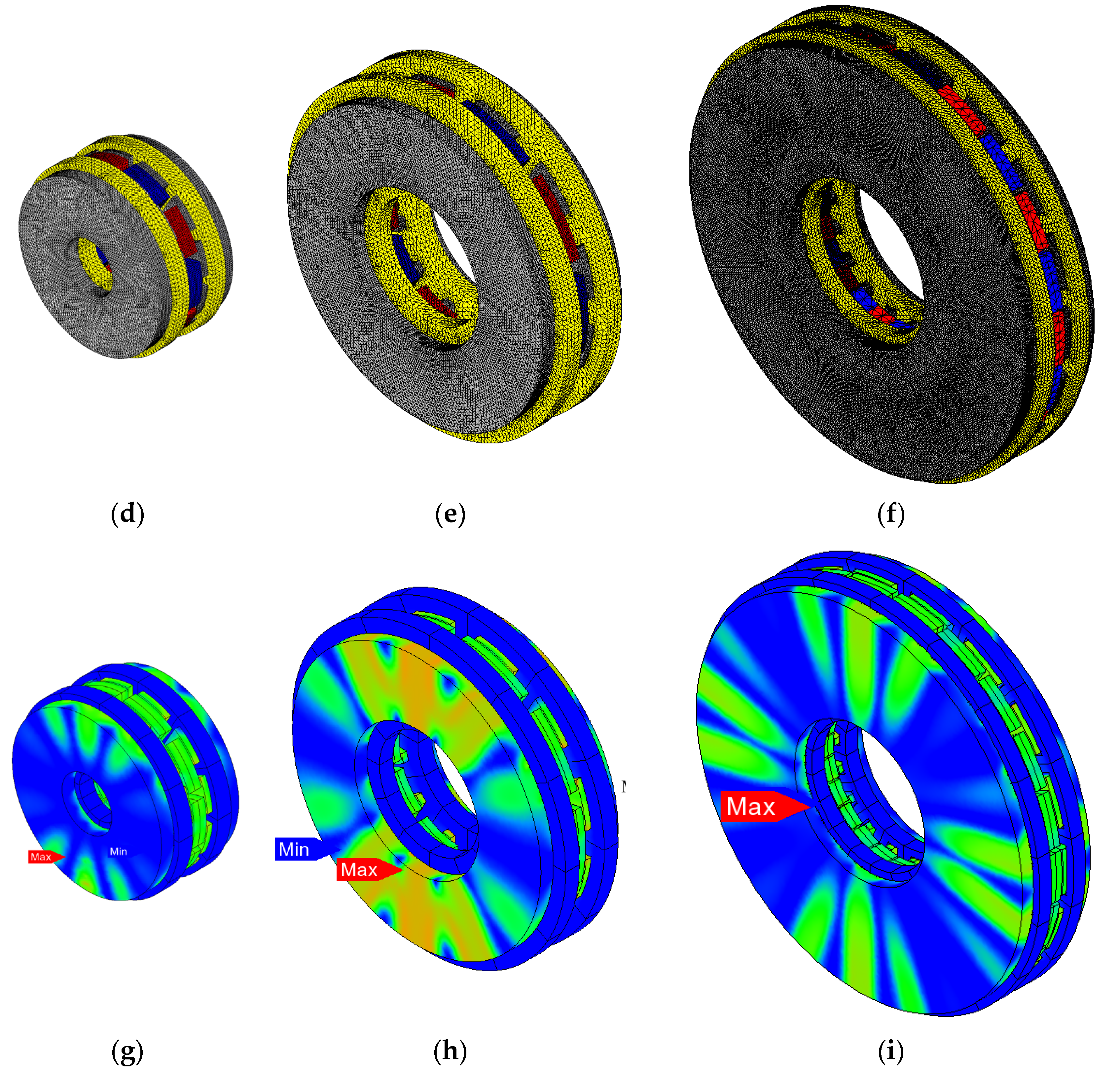
4.9. Validation of Other Random Models

To further validate the effectiveness of the equivalent calculation method proposed in this article, two models of axial flux permanent magnet synchronous motors were randomly added, as shown in Figure 18, and their electromagnetic performance was sequentially calculated using the layered equivalent calculation method. Among them, Motor 1 has a smaller size in the radius direction, a smaller pole arc coefficient, and a higher speed. Motor 2 is the model used for the detailed analysis mentioned earlier, while Motor 3 has a larger radius, a larger pole arc coefficient, and a higher speed. The specific model dimensions and calculation results are shown in

Table 5. Sizes and partial calculation results of three random motor models.

Parameter	Unit	Model-1	Model-2 (Foregoing Analyzed One)	Model-3
Inner radius	mm	20	50	60
Outer radius	mm	60	100	150
Single Stator axial length	mm	27	25	20
Rated speed	r/min	2400	600	1500
Polar arc coefficient	--	0.80	0.83	0.92
Number of poles	--	10	10	22
Number of slots	--	12	12	18
Width of stator slot	mm	8	20	16
Stator slot depth	mm	17	15	12
Fundamental amplitudes of Back-EMF 3D	V	113.52	286.14	285.32
Fundamental amplitudes of Back-EMF 2D	V	114.17	289.08	289.77
error	%	0.57	1.01	1.53
Average torque 3D	N.m	10.76	47.63	105.71
Average torque 2D	N.m	10.85	47.85	107.41
error	%	0.83	1.21	1.58
Core loss 3D	W	83.57	31.69	705.74
Core loss 2D	W	82.34	31.19	696.48
error	%	1.47	1.57	1.33

* All adopt a 9-layer segmented approach.

.

Through the comparison of calculation results, it can be seen that the proposed method has good calculation performance in any size random model. The main electromagnetic performance of the motor, such as no-load back electromotive force, average electromagnetic torque, and stator core loss, are all within 2% of the error, which proves the universality of the calculation method proposed in this paper.

5. Conclusions

To further accelerate the preliminary design and optimization speed of axial flux motors and reduce the computational difficulties, long consumption time, and slow optimization speed caused by three-dimensional finite element simulation, this paper proposes an improved two-dimensional equivalent calculation method. This method has the advantages of fewer variables to be parameterized and simpler simulation settings compared to existing two-dimensional linear motor equivalent methods. The article provides a detailed introduction to the equivalent calculation principle of the proposed method and verifies its feasibility through finite element simulation. The simulation results show that the permanent magnet flux, back electromotive force, electromagnetic torque, and core loss calculated by the proposed method are very close to the 3D finite element simulation results, with low errors within 2%. Although the cogging torque result owns a 7.01% difference, the value is still very close. Moreover, under the same step size and the total number of steps, the calculation time of the proposed method in this paper is minutes, which is only 3% of the 3D finite element simulation. This indicates that the method ensures calculation accuracy while significantly improving the computational efficiency and hardware requirements of axial flux permanent magnet synchronous motors. Although it is not possible to consider the effect of end leakage magnetic flux at the inner and outer radius of the motor, it can already meet the requirements for the initial design of axial flux permanent magnet synchronous motors. It is very suitable for preliminary calculation and rapid optimization of this type of motor and has very good engineering application prospects.

References

1. Tiegna, H.; Bellara, A.; Amara, Y.; Barakat, G. Analytical Modeling of the Open-Circuit Magnetic Field in Axial Flux Permanent-Magnet Machines with Semi-Closed Slots. IEEE Trans. Magn. 2012, 48, 1212–1226. [Google Scholar] [CrossRef]
2. Azzouzi, J.; Barakat, G.; Dakyo, B. Quasi-3-D analytical modeling of the magnetic field of an axial flux permanent-magnet synchronous machine. IEEE Trans. Energy Convers. 2005, 20, 746–752. [Google Scholar] [CrossRef]
3. Gieras, J.F.; Wang, R.J.; Kamper, M.J. Axial Flux Permanent Magnet Brushless Machines; Springer: Dordrecht, The Netherlands, 2004. [Google Scholar]
4. Parviainen, A. Design of Axial-Flux Permanent-Magnet Low-Speed Machines and Performance Comparison between Radial-Flux and Axial-Flux Machines. Ph.D. Thesis, University of Technology, Lappeenranta, Finland, 2005. [Google Scholar]
5. Nguyen, T.D.; Tseng, K.J.; Zhang, S.; Nguyen, H.T. A Novel Axial Flux Permanent-Magnet Machine for Flywheel Energy Storage System: Design and Analysis. IEEE Trans. Ind. Electron. 2011, 58, 3784–3794. [Google Scholar] [CrossRef]
6. Liew, G.S.; Soong, W.L.; Ertugrul, N.; Gayler, J. Analysis and performance investigation of an axial-field PM motor utilising cut amorphous magnetic material. In Proceedings of the 2010 20th Australasian Universities Power Engineering Conference, Christchurch, New Zealand, 5–8 December 2010. [Google Scholar]
7. Kumar, S.; Lipo, T.A.; Kwon, B.I. A 32 000 r/min Axial Flux Permanent Magnet Machine for Energy Storage with Mechanical Stress Analysis. IEEE Trans. Magn. 2016, 52, 1–4. [Google Scholar] [CrossRef]
8. Andriollo, M.; Graziottin, F.; Tortella, A. Design of an Axial-Type Magnetic Gear for the Contact-Less Recharging of a Heavy-Duty Bus Flywheel Storage System. IEEE Trans. Ind. Appl. 2017, 53, 3476–3484. [Google Scholar] [CrossRef]
9. Chen, Q.; Liang, D.; Jia, S.; Ze, Q.; Liu, Y. Analysis of Winding MMF and Loss for Axial Flux PMSM with FSCW Layout and YASA Topology. IEEE Trans. Ind. Appl. 2020, 56, 2622–2635. [Google Scholar] [CrossRef]
10. Liu, Y.; Zhang, Z.; Wang, C.; Geng, W.; Yang, T. Design and analysis of oil-immersed cooling stator with nonoverlapping concentrated winding for high-power ironless stator axial-flux permanent magnet machines. IEEE Trans. Ind. Electron. 2021, 68, 2876–2886. [Google Scholar] [CrossRef]
11. Huang, Y.; Zhou, T.; Dong, J.; Lin, H. Magnetic Equivalent Circuit Modeling of Yokeless Axial Flux Permanent Magnet Machine with Segmented Armature. IEEE Trans. Magn. 2014, 50, 1–4. [Google Scholar] [CrossRef]
12. Zarko, D.; Ban, D.; Lipo, T.A. Analytical Solution for Cogging Torque in Surface Permanent-Magnet Motors Using Conformal Mapping. IEEE Trans. Magn. 2007, 44, 52–65. [Google Scholar] [CrossRef]
13. Driscoll, T.A.; Trefethen, L.N. Schwarz-Christoffel Mapping; Cambridge University Press: Cambridge, UK, 2002. [Google Scholar]
14. Zhu, Z.Q.; Wu, L.J.; Xia, Z.P. An Accurate Subdomain Model for Magnetic Field Computation in Slotted Surface-Mounted Permanent-Magnet Machines. IEEE Trans. Magn. 2010, 46, 1100–1115. [Google Scholar] [CrossRef]
15. Yan, B.; Li, X.; Wang, X.; Yang, Y.; Chen, D. Magnetic Field Prediction for Line-Start Permanent Magnet Synchronous Motor via Incorporating Geometry Approximation and Finite Difference Method into Subdomain Model. IEEE Trans. Ind. Electron. 2023, 70, 2843–2854. [Google Scholar] [CrossRef]
16. Ni, Y.; Jiang, X.; Xiao, B.; Wang, Q. Analytical modeling and optimization of dual-layer segmented Halbach permanent-magnet machines. IEEE Trans. Magn. 2020, 56, 8100811. [Google Scholar] [CrossRef]
Figure 1. A three-dimensional model of an axial flux motor (taking a double stator single rotor motor as an example).
Applsci 13 11748 g001
Figure 2. Flow chart of equivalent method for two-dimensional multi-layer linear permanent magnet synchronous motor.
Applsci 13 11748 g002
Figure 3. Main dimensions of axial flux permanent magnet synchronous motors: (a) axial view; (b) side view.
Applsci 13 11748 g003
Figure 4. Schematic diagram of equivalent method for two-dimensional multi-layer linear permanent magnet synchronous motor.
Applsci 13 11748 g004
Figure 5. Two proportional linear permanent magnet synchronous motor models.
Applsci 13 11748 g005
Figure 6. Comparison of magnetic density distribution between two motor models under the principle of analogy: (a) no-load air gap magnetic flux density in the normal direction; (b) no-load air gap magnetic flux density in the tangential direction; (c) armature reaction air gap magnetic density in the normal direction; (d) armature reaction air gap magnetic density in the tangential direction; (e) magnetic density of iron core teeth; (f) magnetic density of iron core yoke.
Applsci 13 11748 g006aApplsci 13 11748 g006b
Figure 7. Comparison of electromagnetic parameter calculation results between two motor models under the principle of analogy: (a) permanent magnet flux linkage; (b) back electromotive force; (c) thrust force; (d) iron core loss.
Applsci 13 11748 g007
Figure 8. Flow chart of the proposed equivalent method for two-dimensional multi-layer linear permanent magnet synchronous motor.
Applsci 13 11748 g008
Figure 9. Schematic diagram of proposed equivalent method for two-dimensional multi-layer linear permanent magnet synchronous motor.
Applsci 13 11748 g009
Figure 10. Differences between two simplified equivalent methods for axial flux permanent magnet synchronous motors: (a) original method; (b) proposed method.
Applsci 13 11748 g010
Figure 11. A three-dimensional model of a quarter axial flux permanent magnet synchronous motor: (a) grid partitioning result; (b) magnetic density cloud map.
Applsci 13 11748 g011
Figure 12. Equivalent 2D linear permanent magnet synchronous motor model: (a) 2D model, (b) grid partitioning result, (c) magnetic density cloud map.
Applsci 13 11748 g012
Figure 13. Comparison results of permanent magnet flux linkage: (a) waveform; (b) harmonic distribution.
Applsci 13 11748 g013
Figure 14. Comparison results of back electromotive force: (a) waveform; (b) harmonic distribution.
Applsci 13 11748 g014
Figure 15. Comparison results of cogging torque.
Applsci 13 11748 g015
Figure 16. Comparison results of electromagnetic torque.
Applsci 13 11748 g016
Figure 17. The influence of layered numbers on calculation results: (a) fundamental amplitudes of Back-EMF; (b) average torque.
Applsci 13 11748 g017
Figure 18. Three random motor models: On the left is motor 1, in the middle is motor 2, and on the right is motor 3; (ac) schematic diagram of the basic structure; (df) mesh generation result; (gi) results of magnetic density distribution.
Applsci 13 11748 g018aApplsci 13 11748 g018b