Unveiling the Strain Rate Sensitivity of G18NiCrMo3-6 CAST Steel in Tension/Compression Asymmetry

Abstract

This research was devoted to unveiling the strain rate sensitivity (SRS) of G18NiCrMo3-6 cast steel in tension/compression asymmetry. For that purpose, detailed mechanical characterization tests were conducted providing a process window covering quasi-static and medium strain rate regimes (0.001, 0.1, 10 [s⁻¹]) in tension and compression states. Through this experimental effort, the SRS of the material could be extracted by a function of strain and the strain rate which enabled us to create a mathematical expression to easily be implemented as a state variable for constitutive material modeling. Finally, a pressure- and rate-dependent constitutive material model on the basis of the Cocks’89 yield locus definition was created using a subroutine (UMAT) file and the material parameters were verified with respect to the experimental data. The UMAT file also takes into account the tension/compression asymmetry in yielding to handle the effect of the porous media plasticity concept. The predictions of the proposed material model are in line with the experimental outputs.

1. Introduction

The casting process—even though it is probably the most ancient manufacturing process—is still needed and/or provides a powerful alternative in the production of parts which have complex geometries, especially with large dimensions. With proper precautions, large dimensional variations in the cross-sections or large internal cavities do not lead to compelling challenges as in the case of other alternative manufacturing processes. In this regard, cast steel materials are mostly good candidates for the under-body system components of combat vehicles such as suspension arms, steering knuckles, etc., which often have large dimensions and complex geometries. When the demanding design requirements of the defense industry are taken into account, those aforementioned components should also have significant mechanical properties and durability. Therefore, high-strength structural steel castings could find a reasonable area of application in combat vehicle designs. In that sense, the G18NiCrMo3-6 material (conforming to EN 10340:2007) with an ultimate tensile strength (UTS) of nearly 1.0 GPa comes into view for certain engineering designs of under-body systems. While having superior mechanical properties, this material has some drawbacks at the same time. A priori, G18NiCrMo3-6 is a cast steel; thus, it should be treated with a cast iron plasticity approach since it absolutely has a certain amount of porosity. This fact, in turn, eliminates the possibility of modelling this material with the J₂ plasticity theory where the hydrostatic stress does not contribute to yielding and hence there is not any volume change in the plastic range (i.e., the strain tensor is deviatoric by definition). In other words, the hydrostatic stress-dependent yield locus should be constructed with a proper flow rule to model the material behavior of G18NiCrMo3-6. Secondly, this type of cast steel may possess tension/compression asymmetry, i.e., the yield stress and strain hardening behavior differs with respect to tension/compression stress states. This point clearly has to be considered by keeping in mind the fact that some under-body components encounter moment loads in several directions which means that for a specific spatial material point both tensile and compressive stress states may occur interchangeably. In addition, owing to the harsh service-life conditions, under-body components may experience road loads with a wide strain rate spectrum mostly caused by off-road scenarios. (The experimental data, derived from extensive durability tests, indicate a prevalent strain rate regime of 0.001 to 10 (s⁻¹). This finding has shaped the design of our characterization tests.) As in the case of strain hardening, strain rate dependency could also have an asymmetric character which dictates the creation of hydrostatic stress- and rate-dependent constitutive material models that also account for tension/compression asymmetry when aiming to predict the real-life mechanical response of the designed components with high precision. Those aforementioned technical challenges have been extensively investigated by numerous researchers. Perhaps the first attempt to construct a hydrostatic stress-dependent yield function was performed by Drucker and Prager [1]. The Drucker–Prager model is still being used at present; however, it predicts a zero resistance in tension since it was proposed for soil mechanics. Then, Gurson in his pioneering work proposed a hydrostatic stress-dependent yield locus definition which has still been working as a solid basis [2]. Apart from being hydrostatically stress-dependent, the Gurson model was also created in a damage-coupled manner which means that the damage parameter also contributes to the plastic potential which makes it quite appropriate for porous materials [3]. In the specific subfield of cast iron plasticity, tension/compression asymmetric material modeling was also investigated to an intense extent. The most common and appropriate way to handle this asymmetry is to use multiple yield surface definitions [4,5,6,7,8]. The similar and relatively straight-forward application of this kind of modeling strategy is also used by the commercial finite-element software, ABAQUS/Standard. It uses a J₂ plasticity formulation in compression modes; whereas, in tensile stress states, a Rankine-cube-like yield function is defined [9]. In this regard, the studies of Josefson and Hjelm [10] and Metzger et al. [11] have a distinguishing characteristic, which is that they performed a benchmark analysis among existing possible multi-surface yield surface definitions. In particular, there also studies which were devoted to micro-mechanically motivated material models; either they were embedded with unit cells and homogenization or microstructural interactions that were coupled with macro-mechanics [12]. Some of them clearly included detailed microstructural analysis and quantitative metallography as in the studies of Pina et al. [13], Fernandino et al. [14], and Brauer et al. [15]. From this perspective, Cocks has also proposed new hydrostatic yield locus definitions [16] which have certain advantages, especially for industrial applications. The main advantage is that the yield locus definition does not depend on the hardening of the matrix (defect-free portion of the material); thus, the yield definition contains two specific void volume functions which act on macro effective and (von Mises) hydrostatic stress separately. This type of yield expression provides significant ease in mathematical manipulations and especially in partial differentials. Indeed, the need for material parameter extraction is also limited. In industry-driven research, a constitutive model that reduces the need for extensive experimental effort in material parameter extraction and simplifies the time integration scheme—without compromising the complexity of the physical problem—is invaluable. This is particularly important in FEA analyses where computational efficiency is crucial. Therefore, this model (Cocks’89) and some of its derivations are studied in some of the following research [17,18]. Recently, the Cocks’89 model was implemented to assess the mechanical performance of cast aluminum samples by our research group [19]. Moreover, determination of SRS was also performed for various types of materials. However, the SRS-related research generally focused on parameter extraction through experimental methods [20,21,22,23] or theoretical formulations [24,25]. The current contribution differs from those researches in such a way that SRS was experimentally obtained as a function of strain and strain rate and this parameter was buried into the constitutive material model (UMAT file) as a state variable. For that purpose, uni-axial tension and compression tests were conducted for 0.001, 0.1, and 10 (s⁻¹) strain rates using a Gleeble thermo-psychical simulator machine. The necessary data processing procedures were performed aiming to detect the SRS parameter in an asymmetric and rate-dependent fashion. And lastly, these valuable data were coupled with a modified Cocks’89-based formalism to account for rate dependency and tension/compression asymmetry. Although G18NiCrMo3-6 is widely used in engineering designs especially for structural purposes, there is very limited information in the literature, in particular regarding its material parameters. The existing literature data on G18NiCrMo3-6 are mostly related to the empirical and/or theoretical relationship between the process parameters and final mechanical properties [26,27]. This study intends to fill this technical gap which would probably assist any further constitutive modeling efforts henceforth regarding the G18NiCrMo3-6 material. The SRS parameter in tension/compression states is quantified, and an advanced visco-elasto-plastic material model, along with its parameters, is provided for the studied material. To the best of authors’ knowledge, their contribution is unique, offering a validated plasticity model for G18NiCrMo3-6 material that accounts for both asymmetry and rate dependency.

2. Materials and Methods

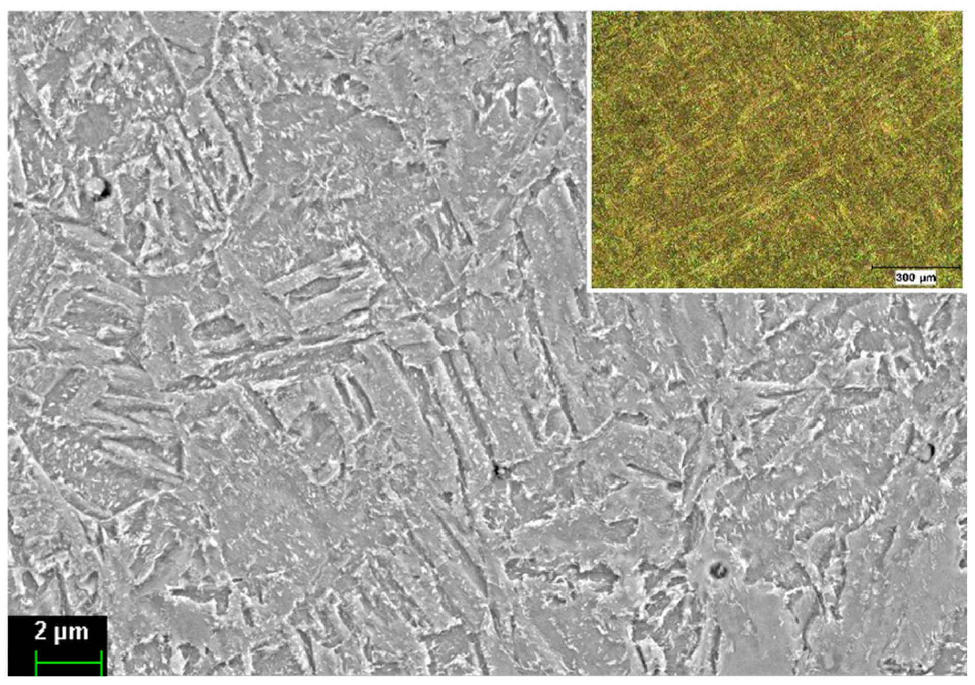
2.1. Studied Material

As indicated in the previous section, the studied cast steel grade is G18NiCrMo3-6. In particular, the material was in QT-1 condition which means that it experienced a conventional quench and tempering QT-1 operation. (QT-1 condition corresponds to a 25 Joule of impact energy requirement in Charpy test at −20 °C in EN 10340 standard) The casting samples had a process route of austenization at 920 °C which was followed with an oil quenching operation. And, as a last step, a tempering process was carried out at 500 °C The chemical composition of the casting samples is also displayed in

Table 1. Chemical composition of G18NiCrMo3-6 (%wt).

C	Si	Mn	Ni	Cr	Mo	Cu	Fe
0.20	0.50	0.90	0.80	0.50	0.45	0.15	Balance

.

Two micrographs of the casted samples can be found in Figure 1, where the tempered martensite-dominant micro-structure could easily be observed at 5000× and 50× magnification. For metallographic inspections, a related sample preparations procedure was applied which consists of several grinding and polishing operations followed by etching with 5% nital solution.

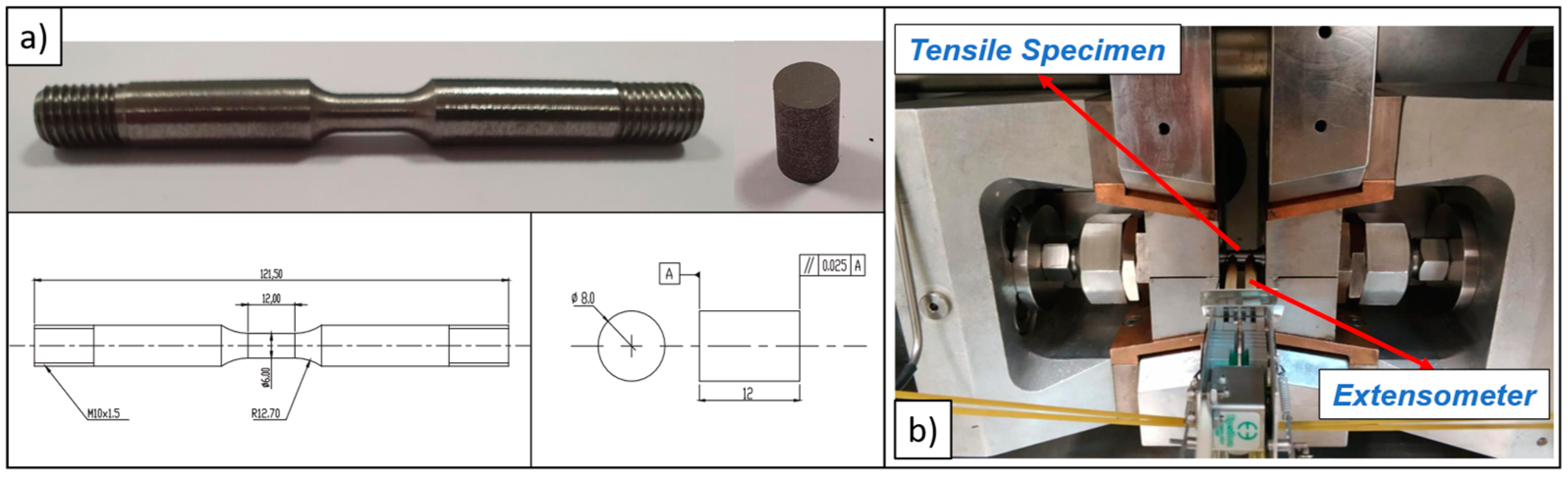
2.2. Mechanical Testing

Mechanical tests were conducted in uni-axial tension and compression conditions at 0.001, 0.1, 10 (s⁻¹) strain rates through a Gleeble-3500 thermo-mechanical simulator machine. For that purpose, cylindrical specimens (ϕ8*12 mm) were manufactured for the compression tests; meanwhile, dog-bone cylindrical specimens having an initial gauge length of 12 mm were used in tensile testing. The specimens were manufactured while having a good surface finish quality, especially the compression test specimens processed through grinding operations to assure the necessary parallelism between the frontal faces. The technical drawings and real pictures of the specimens are shown in Figure 2. Furthermore, aiming to increase the precision in the strain measurement, a tactile extensometer was implemented for tensile tests at 0.001 and 0.1 (s⁻¹) strain rates. Apart from those tests, the strain values were computed on the basis of conventional cross-head displacement data. A test set-up image with the extensometer installation is shown in Figure 2. All mechanical tests were performed 3 times to ensure the consistency of results. The whole data of mechanical tests were submitted at Section 4.1.

Thanks to the fully integrated digital closed-loop control system of the Gleeble-3500, the strain rate during the whole deformation process could be monitored and controlled with high precision. The true stress vs. true strain data were able to be created by the test machine. As can be seen in Figure 3, the results are assessed as satisfactory.

Afterwards, a specific code was created in the MATLAB^® environment to compute the yield stresses for the whole tests. To achieve this, the conventional offset stress ($R_{p0.2}$) method was used. Sample data regarding this computation method were illustrated, and the computed yield stress value is provided in Figure 4.

2.3. Determination of SRS

After obtaining the strain–stress response at specific strain rates, these data were processed properly to obtain the SRS parameter (as a general convention of theory of plasticity, SRS parameter is often denoted as m parameter). When a power-law-based strain rate effect (Equation (1)) is used [28], then parameter m can be automatically obtained via processing of two plastic responses at distinct strain rates. (Readers should give attention to the fact that the first component of Equation (1) is the rate-independent hardening functions, and the second term contributes to the rate sensitivity effect). In other words, when two flow curves are present (in general, one of them is the reference train rate data), it is possible to determine m with the help of Equation (2) [23,29]:

$$\sigma =\gamma \left({\epsilon }_p\right)\times {\left(\frac{\dot{{\epsilon }_p}}{\dot{{\epsilon }_0}}\right)}^m$$

(1)

$${\left.m\right|}_{({\epsilon }_0, \dot{{\epsilon }_p})}=\frac{\partial \mathit{ln}\left(\frac{{\sigma }_1}{{\sigma }_0}\right)}{\partial \mathit{ln}\left(\frac{\dot{{\epsilon }_1}}{\dot{{\epsilon }_0}}\right)}$$

(2)

In Equation (1), $\dot{{\epsilon }_p }$ is the strain rate which is apart from the reference strain rate $\dot{{\epsilon }_0}$. Within the scope of this contribution, $\dot{{\epsilon }_0}$ was taken as 0.001 (s⁻¹), in the same way as the general rule-of-thumb of plasticity, which is based on the fact that beyond this limit materials do mostly not possess any rate dependency. Furthermore, in Equation (2), ${\sigma }_{0 }$ and ${\sigma }_1$ are experimentally obtained true stress values which correspond to the same strain value at the strain rates of $\dot{{\epsilon }_0}$ and $\dot{{\epsilon }_1}$, respectively.

As can be observed in Equation (2), m is not constant, and it is generally a function of the plastic strain and strain rate. However, it is still possible to obtain it with proper data processing operations. This task is also fulfilled by a specific MatLab^® code. Since the experimental data were obtained with high frequency (may reach up to 10⁵ Hz), a linear interpolation approach was accepted as a proper solution. While using the above-mentioned formulation and the procedure, m was determined regarding tension and compression asymmetry, as in Figure 5. The built-in function interp1 of MatLab^® and the above-mentioned formulation were used, for that purpose (in order to capture the asymmetry of SRS in tension and compression zones, m was computed separately for the designated stress states specifically). The obtained m parameter data were depicted as an advanced version (surface data) at Section 4 since they create a 3D surface through having two independent variables).

3. Results

3.1. Basic Formulation

The yield locus was defined in the Cocks’89 material model as in Equation (3):

$$\varphi =\underset{\stackrel{-}{\sigma }}{\underbrace{\sqrt{\frac{{\sigma }_{eq}^2}{{\mathrm{g}}_1\left(f\right)}+\frac{{\sigma }_m^2}{{\mathrm{g}}_2\left(f\right)}}}}-{\sigma }_y=0$$

(3)

In Equation (3), ${\sigma }_{eq}$ is the equivalent von Mises stress and ${\sigma }_m$ is the mean stress which were explicitly given in Equation (4); moreover, ${\mathrm{g}}_1$ and ${\mathrm{g}}_2$ are functions of f which is nothing but the void volume fraction; and finally $\varphi$ is the yield potential. In particular, $\stackrel{-}{\sigma }$ is the equivalent stress definition of the Cocks’89 plasticity model:

$${\sigma }_{eq}=\sqrt{\frac{3}{2}{\mathit{S}}_{\mathit{i}\mathit{j}}{\mathit{S}}_{\mathit{i}\mathit{j}}} , {\sigma }_m=\frac{{\sigma }_{kk}}{3}$$

(4)

In Equation (4) σ is the (Cauchy) stress tensor and $S_{ij}$ is the deviatoric part of it (please note that Einstein’s summation convention is in place for the formulation). Therefore, ${\sigma }_{kk}$ is actually a scalar value and equals to $I_1$ which is the first invariant of the stress tensor (aiming to eliminate any possible confusions, the tensorial expressions were designated by bold character to be easily distinguished from scalar quantities). To clarify the yield locus definition in Cocks’89, the two separate functions of f were also provided in Equation (5). As expected, when $f\to 0,$ i.e., void volume fraction is zero (conventional metal plasticity approach), the yield locus definition turns out to the von Mises yield criteria $\left[\sqrt{3J_2}-{\sigma }_y=0\right]$:

$${\mathrm{g}}_1=\frac{{\left(1-f\right)}^2}{1+\frac{2}{3}f}, {\mathrm{g}}_2=\frac{2}{9}\frac{\left(1+f\right){\left(1-f\right)}^2}{f}$$

(5)

By assuming the associative flow rule, the plastic strain rate equation can be written as Equation (6). (Similar to the conventional computational plasticity approach, Equation (6) was constructed as a time rate of change form since the analyses are conducted via a time integration scheme).

$$\dot{{\epsilon }_p}=\dot{\lambda } \underset{{\mathit{N}}_p}{\underbrace{\frac{\partial \varphi }{\partial \sigma }}}$$

(6)

In Equation (6), ${\epsilon }_p$ is the plastic strain tensor, $\lambda$ is the plastic multiplier and ${\mathit{N}}_p$ is the unit normal vector of the plastic flow, while the dot operator denotes the time derivative of the tensors (unit normal vector was shown via a capital letter to eliminate the confusion with n and n + 1 subscripts of time integration). By taking the partial derivative of Equation (4), reads as (Equation (7)):

$${\mathit{N}}^p=\left(\frac{3}{2}\frac{{\mathit{S}}_{\mathit{i}\mathit{j}}}{{(\mathrm{g}}_1\stackrel{-}{ \sigma })}+\frac{1}{9}\frac{{\sigma }_{kk}}{{(\mathrm{g}}_2 \stackrel{-}{\sigma })}\mathbf{I}\right)$$

(7)

In this study, a Euler backward time integration scheme was used, then N^p calculation (Equation (8)) dictates under Equation (7), where $\mathbf{I}$ is the second order identity tensor:

$${\mathit{N}}_{n+1}^p=\left(\frac{3}{2 }\frac{ {\left({\mathit{S}}_{\mathit{i}\mathit{j}}\right)}_{n+1}}{{(\mathrm{g}}_1 {\stackrel{-}{\sigma }}_{n+1})}+\frac{1}{9}\frac{{ \left({\sigma }_{kk}\right)}_{n+1}}{ {(\mathrm{g}}_2 {\stackrel{-}{\sigma }}_{n+1})}\mathbf{I}\right)$$

(8)

By combining Equations (6) and (8), one can obtain the plastic strain tensor at the end of time increment as (Equation (9)):

$${\epsilon }_{n+1}^p=\underset{\dot{\lambda }dt}{\underbrace{\mathsf{\Delta }\lambda }}{\mathit{N}}_{n+1}^p$$

(9)

Equation (9) can also be written in a scalar form as Equation (10), where ${\stackrel{-}{\epsilon } }^p$ denotes equivalent plastic strain:

$${\stackrel{-}{\epsilon } }_{n+1}^p=\mathsf{\Delta }\lambda {\mathit{N}}_{n+1}^p+{\stackrel{-}{\epsilon } }_n^p$$

(10)

On the other hand, with the assumption of incompressible plastic flow of the defect-free matrix material (without any porosity), the only contribution to volume change is the change in porosity level. Then, the accumulation of porosity level can directly be linked to the non-isochoric portion of strain tensor, as indicated in Equation (11) (this assumption omits the contribution of elastic strains to volume change, but it is still a proper strategy since elastic strains are extremely small compared to plastic counterparts, especially in moderate strain regime).

$$\dot{f}=\left(1-f\right)\times {\dot{\epsilon }}_{kk}$$

(11)

Again, the similar convention of Equation (9), f was defined at the end of the time increment as Equation (12):

$$f_{n+1}=f_n+\left[(1-f_{n+1})\left({{\dot{\epsilon }}_{kk}}_{n+1}\right)\right]\mathsf{\Delta }t=f_n+(1-f_{n+1}){\left({\mathsf{\Delta }\mathsf{\epsilon }}_{kk}\right)}_{n+1}$$

(12)

By necessary mathematical manipulations, finally Equation (12) converts to Equation (13):

$$f_{n+1}=\frac{f_n+{\left({\mathsf{\Delta }\mathsf{\epsilon }}_{kk}\right)}_{n+1}}{1+{\left({\mathsf{\Delta }\mathsf{\epsilon }}_{kk}\right)}_{n+1}}$$

(13)

Combining Equation (12), Equations (8) and (13) finally yields Equation (14) for $f_{n+1}$:

$$f_{n+1}=\frac{f_n+\mathsf{\Delta }\lambda \left[\frac{1}{3}\frac{{\left({\sigma }_{kk}\right)}_{n+1}}{{ \left({\mathrm{g}}_2\right)}_n {\stackrel{-}{\sigma }}_{n+1}}\right]}{1+\mathsf{\Delta }\lambda \left[\frac{1}{3}\frac{{\left({\sigma }_{kk}\right)}_{n+1}}{{ \left({\mathrm{g}}_2\right)}_n{\stackrel{-}{ \sigma }}_{n+1}}\right]}$$

(14)

Equation (14) also means that at the end of time increment, when the stress and strain update is conducted, f can also be determined. Thus, the f parameter was processed like a state variable. Sticking to elastic predictor–plastic update methodology of computational plasticity, ${\stackrel{-}{\sigma }}_{n+1}$ can be written in an open form as (Equation (15)):

$${\sigma }_{n+1}=2G\left[ dev\left({\epsilon }_{n+1}\right)-dev\left({\epsilon }_{n+1}^p\right) \right]+\kappa \left[ tr\left({\epsilon }_{n+1}\right)-tr\left({\epsilon }_{n+1}^p\right) \right] \mathbf{I}$$

(15)

In Equation (15), G is the shear and $\kappa$ is the bulk modulus; in addition, dev and tr represent the deviatoric part and trace of the tensors, respectively. Combining Equations (8), (9) and (15) yields (Equation (16)) for ${\sigma }_{n+1}$:

$$\begin{gathered} {\sigma }_{n+1}=2G\left[ dev\left({\epsilon }_{n+1}\right)-dev\left({\epsilon }_n^p\right)-\mathsf{\Delta }\lambda \frac{ 3}{ 2} \frac{dev\left({\sigma }_{n+1}\right)}{{ \left({\mathrm{g}}_1\right)}_n{\stackrel{-}{ \sigma }}_{n+1}} \right]+\kappa [ tr\left({\epsilon }_{n+1}\right)-\dots \\ \dots tr\left({\epsilon }_n^p\right)-\frac{1}{3} \frac{tr\left({\sigma }_{n+1}) \mathsf{\Delta }\lambda \right)}{{ \left({\mathrm{g}}_2\right)}_n{\stackrel{-}{ \sigma }}_{n+1}}] \mathbf{I} \end{gathered}$$

(16)

By rearranging and conducting necessary mathematical manipulations, Equation (16), ${\sigma }_{n+1}$ can be decomposed as Equations (17) and (18):

$$dev({\sigma }_{n+1})=\frac{2G [ dev\left({\epsilon }_{n+1}\right)-dev\left({\epsilon }_n^p\right)]}{1+\frac{3G\mathsf{\Delta }\lambda }{{ \left({\mathrm{g}}_1\right)}_n{\stackrel{-}{ \sigma }}_{n+1}}}$$

(17)

$$tr({\sigma }_{n+1})=\frac{3\kappa [ tr\left({\epsilon }_{n+1}\right)-tr\left({\epsilon }_n^p\right)]}{1+\frac{\kappa \mathsf{\Delta }\lambda }{{ \left({\mathrm{g}}_2\right)}_n{\stackrel{-}{ \sigma }}_{n+1}}}$$

(18)

With the help of Equations (3) and (18), the yield locus definition for the plastic increment can be formulated as Equation (19). For the simplicity of formulation, the nominators of Equations (17) and (18) (expressions in blue color) were termed as P and Q, respectively.

$${\varphi }_{n+1}=\sqrt{\frac{3 }{2 }\frac{\left[{dev(\sigma }_{n+1}\right) : {dev(\sigma }_{n+1}\left)\right]}{{ \left({\mathrm{g}}_1\right)}_n}+\frac{1 }{9 }\frac{\left[{{tr}^2(\sigma }_{n+1}\right)]}{{ \left({\mathrm{g}}_2\right)}_n}}$$

(19)

The basic motivation behind Equation (19) is to formulate the yield locus as a function of incremental plastic multiplier ($\mathsf{\Delta }\lambda$). One can easily observe that in Equation (19) the first term was composed of all known quantities. In other words, the only unknown in Equation (19) is the incremental plastic multiplier (please note that ${\stackrel{-}{\sigma }}_{n+1}=f\left(\mathsf{\Delta }\lambda \right)$). By means of the equilibrium condition (${\varphi }_{n+1}=0$) and the trial stress (elastic predictor) formulation (Equation (21)), Equation (19) can be reconstructed as Equation (20) via leaning to co-axiality principle (Equation (22)), meaning that trial and Cauchy stress tensors have the same unit outward normal direction:

$${\varphi }_{n+1}=\sqrt{\frac{{\mathit{S}}_{n+1}^{trial} : {\mathit{S}}_{n+1}^{trial}}{{ \left({\mathrm{g}}_1\right)}_n{ P}^2}+\frac{1 }{9 }\frac{{\left[{\sigma }_{n+1}^{trial}\right]}^2}{{ \left({\mathrm{g}}_2\right)}_n Q^2}}-{\left({\sigma }_y\right)}_{n+1}=0$$

(20)

$${\sigma }_{n+1}^{trial}=2G \left[ dev\left({\epsilon }_{n+1}\right)-dev\left({\epsilon }_n^p\right) \right]+\kappa \left[ tr\left({\epsilon }_{n+1}\right)-tr\left({\epsilon }_n^p\right)\right] \mathbf{I}$$

(21)

$${\mathit{N}}_{n+1}^p={\mathit{N}}_{trial}^p$$

(22)

The fact that Equation (20) is a non-linear equation of one unknown, it could be solved by means of numerical methods. In this contribution, the Newton–Raphson method was engaged to solve Equation (20) with a convergence criteria of 10⁻⁶.

The details of the time integration scheme in UMAT subroutine are given in the following section.

3.2. Time Integration Procedure

The UMAT subroutine runs as follows:

• Initialization: Uptake the material parameters, state variables, and the deformation gradient (F) at beginning of the time increment.
• Computation of strain tensor: Compute the Hencky strain tensor through the use of F (our code was constructed as finite-strain basis in such a way that free body translations were eliminated by means of Hencky strain measure [30], however Kroner decomposition [31] was discarded for the present study). Hencky strain measure is one of the most appropriate ways to deal with moderate deformations [32].
• Check the plasticity criterion: Compute the trial stress (Equation (21)) and check for the yield locus definition (Equation (23)):

  $${\varphi }_{trial}=\sqrt{\frac{{\mathit{S}}_{n+1}^{trial} : {\mathit{S}}_{n+1}^{trial}}{{ \left({\mathrm{g}}_1\right)}_n}+\frac{1 }{9 }\frac{{\left[{\sigma }_{kk}^{trial}\right]}^2}{{ \left({\mathrm{g}}_2\right)}_n }}-{\left({\sigma }_y\right)}_n\le 0$$

  (23)
• Update state variables:
  If ${\phi }_{trial}$ ≤ 0 → step is elastic (∆λ = 0) thus, conserve the state variables.
  If ${\phi }_{trial}$ > 0 → step is plastic, solve for ∆λ (Equation (20)). Update ${\sigma }_{n+1}$, ${\epsilon }_{n+1}^p$, $f_n$, $m_n$.
• Finalization: Deliver the state variables and tangent modulus to Abaqus solver for the convergence check. For the present study, perturbation-based numerical tangent matrix formulation is used. (Equation (24)):

  $$C_{ij,n+1}=\frac{{∆\sigma }_{i,n+1}}{{∆\epsilon }_{j, n+1}}$$

  (24)

3.3. Imposing the Asymmetry and Rate Dependence

The tension/compression asymmetry and rate dependence contribute to the computation of flow through incremental plastic multiplier as Equation (20). In particular, the experimentally obtained material parameters differ where the state of stress behaves as a switching parameter. This fact is explained through the mathematical expressions below Equation (24):

$${\sigma }_y=\left[{\sigma }_0+B {\left({\stackrel{-}{\epsilon }}^p\right)}^{r^{*}}\right] {\left(\frac{\dot{{\epsilon }_p}}{\dot{{\epsilon }_0}}\right)}^{m^{*}}$$

(25)

where $r^{*}$ is defined as in Equation (25). Likewise, ${\sigma }_0$ and $m^{*}$ were determined separately regarding tension and compression conditions:

$$r^{*}=\left\{\begin{array}{c}{r}_{t } for tension r_{t }\in N\\ r_c for compression r_{c }\in N\end{array}\right.$$

(26)

Then, Equation (24) could be rewritten as Equation (26) (please note that $∆t$ is a known scalar quantity which is delivered via the Abaqus solver).

$${\sigma }_y=\left[{\sigma }_0+B {\left({{\stackrel{-}{\epsilon }}^p}_n+\mathsf{\Delta }\lambda \right)}^{r^{*}}\right] {\left(\frac{\mathsf{\Delta }\lambda }{∆t \dot{{\epsilon }_0}}\right)}^{m^{*}}$$

(27)

4. Results and Discussion

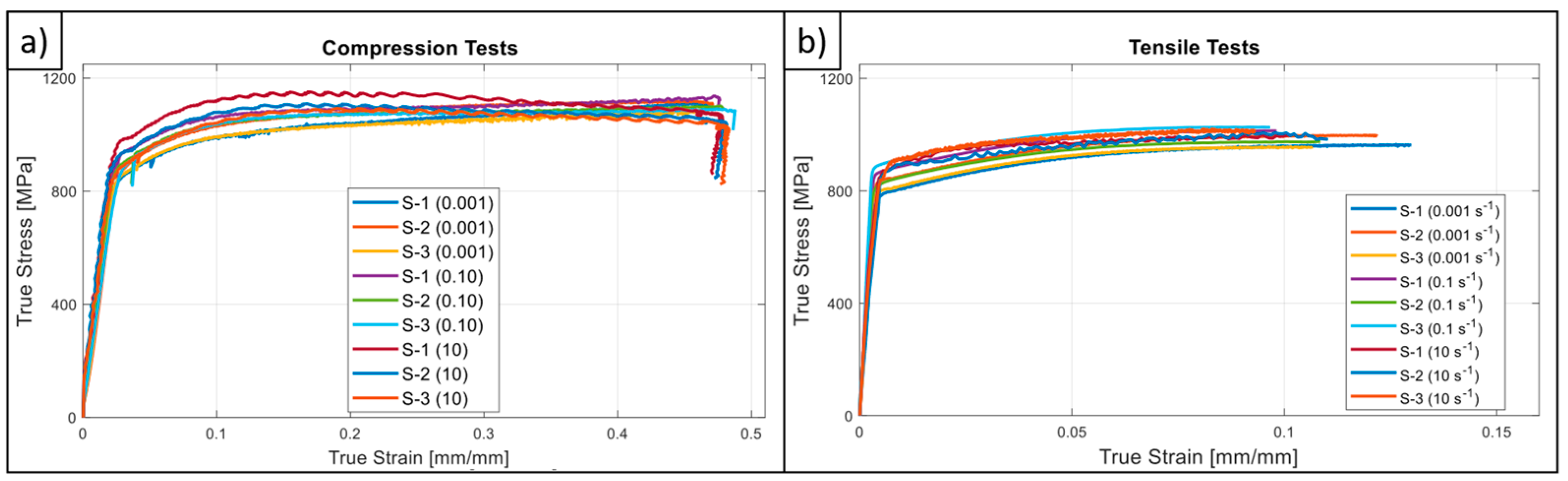
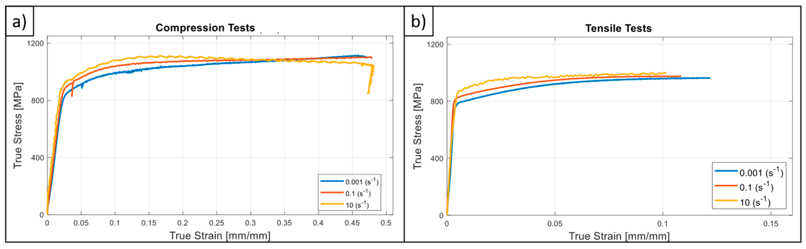
4.1. Mechanical Testing

The obtained Gleeble test results (whole set) are depicted in Figure 6.

Moreover, in order to perform the necessary curve fitting operation which was proposed in Equation (24), the flow curves (true plastic strain vs. true stress) at the reference strain rate were extracted with data processing. At first glance, the Ludwik equation [33] (${\sigma }_y={\sigma }_0+{B\epsilon }_p^n$) suits the experimental data quite well. Therefore, this formalism was used to model the flow curve behavior. The flow curves and fitted parameters of the Ludwik equation are shown in Figure 7 for the compression mode. The explained data processing procedure was also conducted for tensile tests and the computed parameter set is provided in

Table 2. Extracted parameters from curve fitting operations (standard deviation values were indicated in parentheses).

	${\mathsf{\sigma }}_0 (0.001 {\mathbf{s}}^{-1})$	${\mathsf{\sigma }}_0 (0.1 {\mathbf{s}}^{-1})$	${\mathsf{\sigma }}_0 (10 {\mathbf{s}}^{-1})$	B	n
Compression	815.64 (±1.93%)	862.79 (±1.89%)	882.18 (±2.89%)	368.20	0.2798
Tension	808.65 (±2.70%)	858.73 (±2.84%)	876.80 (±1.36%)	551.30	0.5075

.

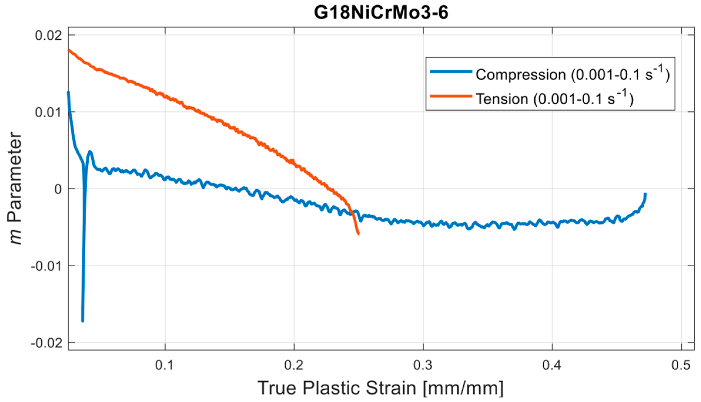
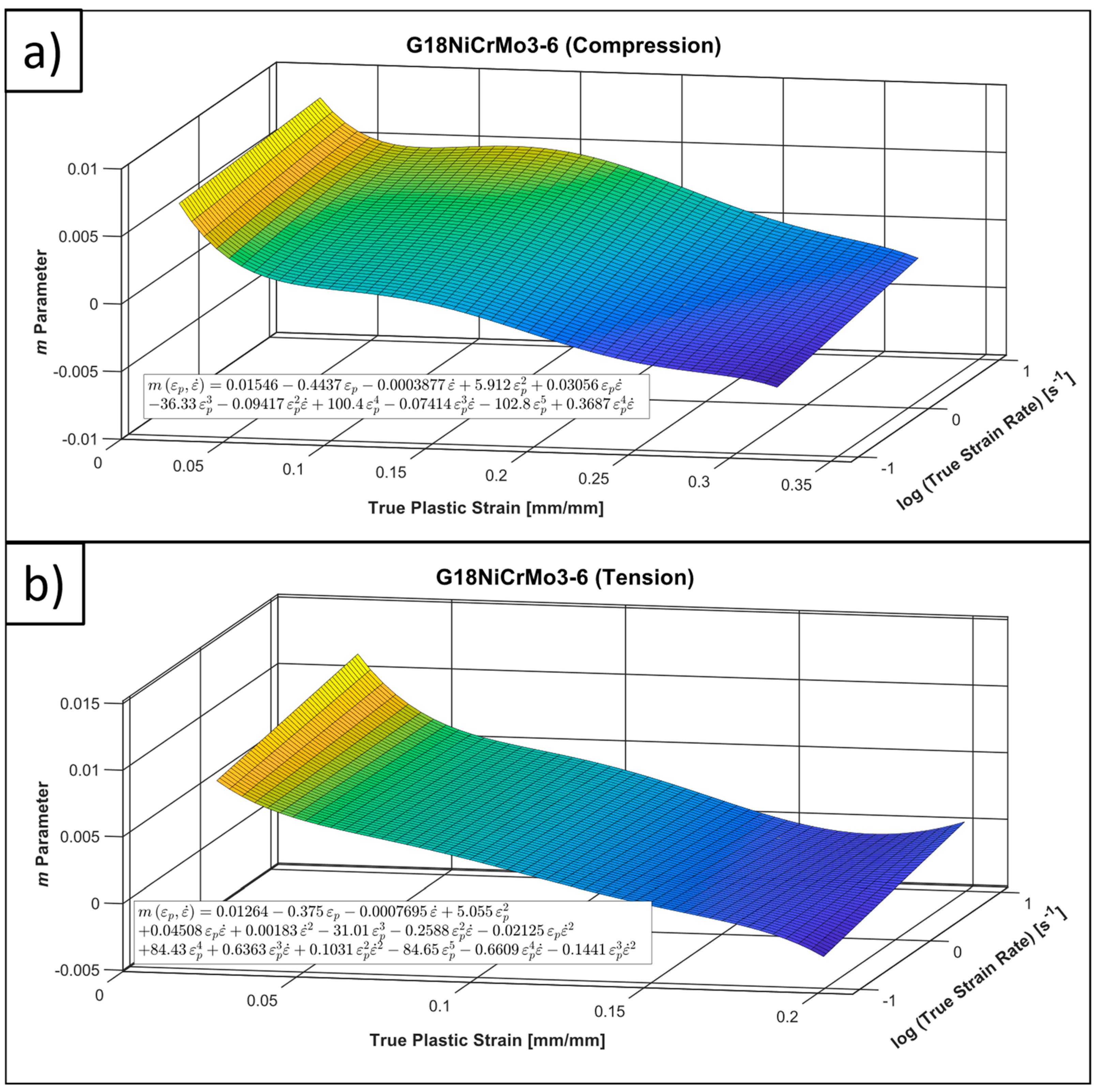
4.2. Determination of SRS

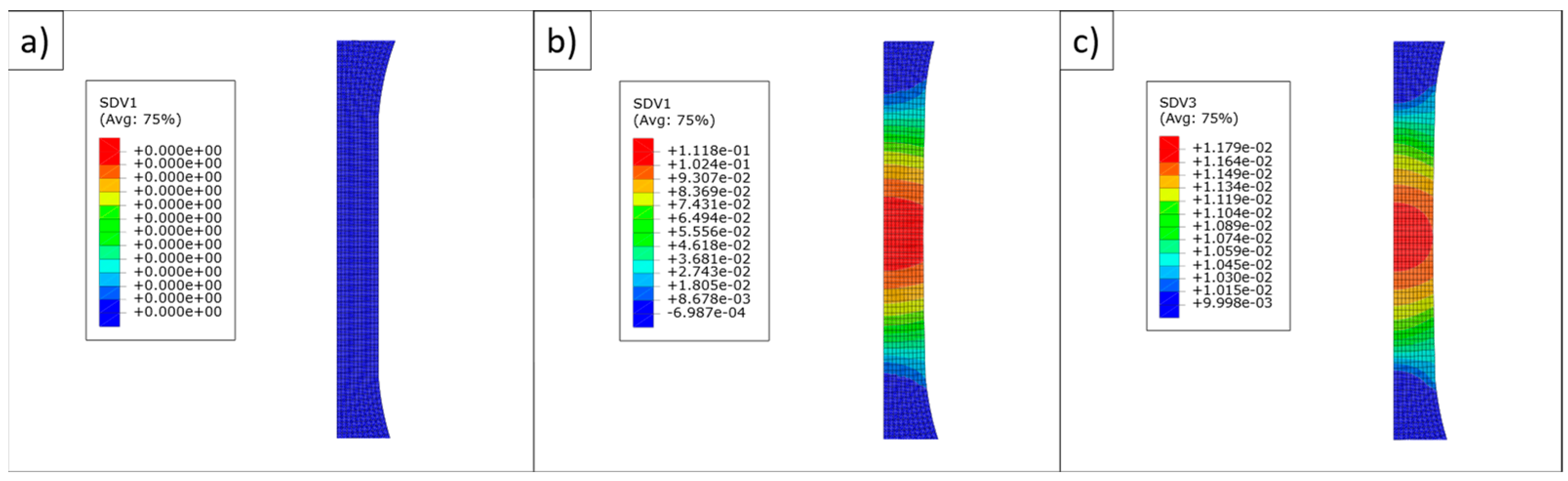
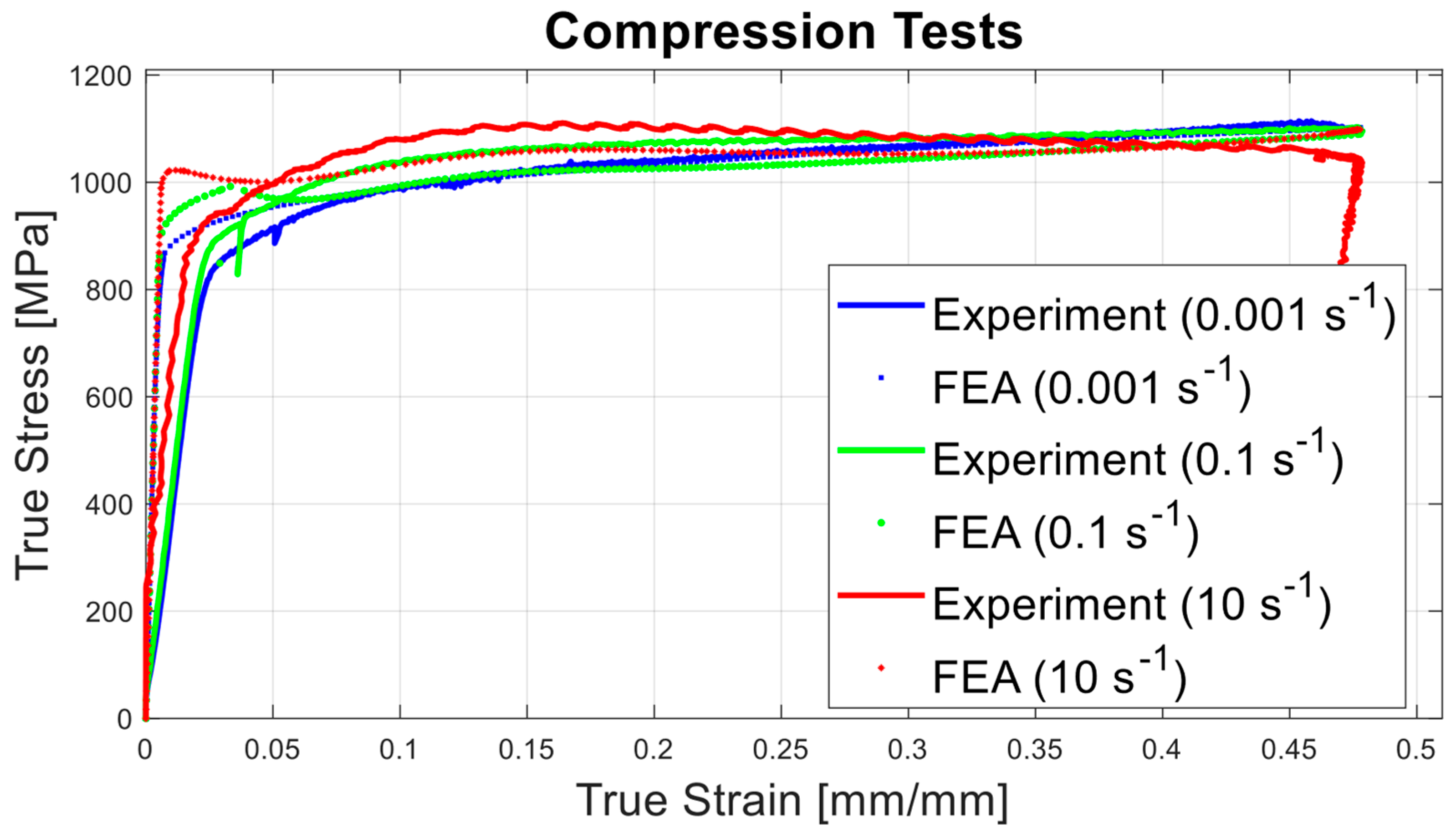
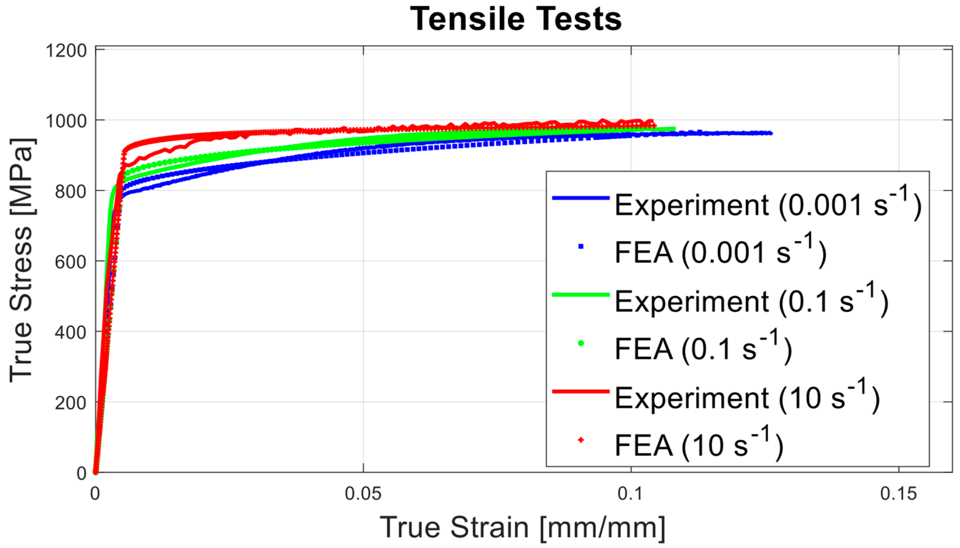
After conducting the mechanical tests, the SRS parameter was calculated with the aforementioned methodology. The obtained SRS behavior is constructed as a surface plot in Figure 8, aiming to display the distinct behavior in compression/tension asymmetry, The experimental results (only the mid-valued ones) are depicted in Figure 9.

In Figure 8 and Figure 9, as a first observation, it could be stated that the studied material has a dominantly saturation-type plastic response. This character is more dominant for moderate strain rates. Secondly, the strain rate dependence can also be detected in both stress states which is more effective in the near-yielding zone. With the increasing plastic strain, the rate sensitivity diminishes and even turns out to be negative. In other words, G18NiCrMo-3-6 shows a strain softening effect at moderate strain rates compared to the quasi-static condition. This fact was interpreted as an adiabatic heating-induced thermal softening effect. This finding agrees well with the previous literature data [34,35,36]. Since the studied material could be accepted as a high-strength metal by having a UTS nearly 1.0 GPa, there is a significant amount of inelastic energy introduced to the system during the deformation process. In our view, this is the basic reason behind the strain softening phenomena after moderate strain values (i.e., ${\epsilon }_p\ge 0.30$). Since the obtainable strain values are much higher for compression tests, this strain softening is modest on the tension side. In addition, it is also worth emphasizing that there is also a slight change in yield stress for tension/compression asymmetry, as expected. The compressive yield stress is bigger than the tensile one of 4%. As a result, separate characters of SRS parameter were quantified and the analytical formulations are also provided in Figure 8. The strain softening character in high strain value at compression tests yields a negative SRS phenomena. Therefore, in high strain rate in compression, the material at the onset of plastic deformation exhibits rate sensitivity unlike the moderate strain values. This type of flow stress character cannot be precisely predicted using the conventional approach of the Johnson–Cook plasticity [37] model where the flow curve is raised or lowered via a constant multiplier term.

4.3. FEA Models

The experiments were reproduced in Abaqus environment with the created UMAT subroutine. Based on the axi-symmetric nature of the conducted mechanical tests, the FEA models were modeled by CAX8R elements (biquadratic, quadrilateral element with reduced integration) in 2D condition. The experimentally obtained time vs. displacement data was given as a boundary condition to the upper face while providing an encastre (zero rotation and translation) condition at the lower face of the specimens. With this type of modeling, the rate effect can be introduced to the FEA model under the circumstances of sticking to the SI unit system. In this perspective, the elasto-plastic behavior of the material is numerically obtained, and the results were compared with the experimental findings. Keeping in mind the condition that (i) tensile tests were modeled up to diffuse necking and (ii) in compression tests the barreling effect is neglected (i.e., without any friction effect), the total deformations are both homogeneous in the compression specimen and the gauge zone of the tensile specimen. In fact, the stress values, and the evolution of the porosity level (f) were able to be computed by the code (in that sense, the analysis can be modeled by one element test without sacrificing the precision of results; however, a stable meshing was applied on the geometries to be ready for upcoming efforts regarding instable plastic flow region). An average element size is applied as 0.25 × 0.25 mm. This UMAT file intended to be modified and enhanced to capture the response in instability region or even in fracture through improving the formulation of void volume fraction and coupling it with any damage model approach. In Figure 10, some results in calculated stress, equivalent plastic strain, and porosity evolution values are depicted, in a detailed manner. Similarly, the mesh structure and the equivalent plastic strain and f parameter at the end of analysis is provided for the tensile test at 0.001 s⁻¹ in Figure 11. Furthermore, in Figure 11, the comparison of experimental and numerical results is provided. These reveal that the proposed material constitutive model succeeds in capturing pressure, rate dependent, and asymmetric plastic behavior of the G18CrNiMo3-6 material. For FEA analysis, the initial void volume fraction was taken as 0.010 (Figure 12 and Figure 13).

5. Conclusions

In this study, the SRS of the G18NiCrMo3-6 cast steel material was experimentally obtained including tension/compression asymmetry. For that purpose, a specific set of mechanical tests was carried out at distinct strain rate conditions. By means of this experimental effort, power-law-based strain rate-dependent flow behavior was determined and the necessary material parameters were extracted and shared with readers. To better capture SRS, the m parameter was formulated as strain, strain rate, and asymmetry-dependent fashion. In particular, two surface plots of the SRS parameter were provided with their analytical expressions regarding tension and compression stress states which is sufficient to construct an advanced visco-elasto-plastic material model for the studied material. Finally, the aforementioned material model parameters were embedded to a pressure- and rate-dependent constitutive model by means of a UMAT file. Moreover, the proposed Cocks’89-based model was verified 336 with the experimental data. The following outputs could be extracted from the current contribution:

• The G18NiCrMo3-6 material possess an asymmetric yielding character, in other words, it yields stress in compression at a rate 4% bigger than the tensile one.
• Indeed, the strain hardening and SRS character is also quite asymmetric for the studied material. This fact was quantified with the help of power-law-based flow stress formulation and the determination of the m parameter. From a general point-of-view, SRS is more dominant in the tensile direction; however, it has a decreasing tendency with increasing strain as in the compressive stress states. In the view of the authors’, the shared material data within this study provide an important resource for the upcoming research activities on G18NiCrMo3-6 about which the existing literature data are extremely limited.
• Unlike the tensile test in a medium-strain rate regime, strain softening phenomena were observed in compression tests which were interpreted as the effect of adiabatic heating. Owing to this finding on the compression side, the material exhibits a rate sensitivity character up to a certain strain value but then the strain softening effect contributes to the plastic response. This fact can be handled through defining SRS parameters as a function of strain as in the proposed constitutive model. On the contrary, a conventional Johnson–Cook type formalism cannot catch up with these phenomena where the effect of rate contribution is formulated through a constant multiplier term.
• The created constitutive model (UMAT file) runs without any problem which was formulated on a finite strain basis and uses implicit time integration scheme. This UMAT file could easily serve in inspecting the effect of material parameters (like the initial void volume fraction, etc.) on the macro-mechanical performance of any design which is made up of G18NiCrMo3-6. However, it is also noteworthy that in the proposed model, the void growth is just linked to the volumetric strains, meaning that any void coalescence effect is not included in the formulation. Indeed, this fact may also give rise to precision loss especially in a low-stress triaxiality regime.
• In our view, the present material model and the verified parameter set significantly enhance the technical knowledge level related to the G18NiCrMo3-6 material and would serve as a solid basis for the upcoming research studies. Our efforts will focus on creating proper coupling between the estimated void volume fraction and any appropriate damage rule to improve the proposed model which would account for both damage, void coalescence, and localization phenomena. Furthermore, plasticity-induced heating would also be studied to estimate the strain softening behavior via proper thermo-coupled plasticity formulations.

References

1. Drucker, D.C.; Prager, W. Soil mechanics and plastic analysis or limit design. Q. Appl. Math. 1952, 10, 157–165. [Google Scholar] [CrossRef]
2. Gurson, A.L. Continuum Theory of Ductile Rupture by Void Nucleation and Growth: Part I—Yield Criteria and Flow Rules for Porous Ductile Media. J. Eng. Mater. Technol. 1977, 99, 2–15. [Google Scholar] [CrossRef]
3. Trillat, M.; Pastor, J. Limit analysis and Gurson’s model. Eur. J. Mech. A/Solids 2005, 24, 800–819. [Google Scholar] [CrossRef]
4. Coffin, L.F.J. The Flow and Fracture of a Brittle Material. J. Appl. Mech. 2021, 17, 233–248. [Google Scholar] [CrossRef]
5. Wiese, J.W.; Dantzig, J.A. Modeling stress development during the solidification of gray iron castings. Metall. Trans. A 1990, 21, 489–497. [Google Scholar] [CrossRef]
6. Hjelm, H.E. Yield Surface for Grey Cast Iron Under Biaxial Stress. J. Eng. Mater. Technol. 1994, 116, 148–154. [Google Scholar] [CrossRef]
7. Altenbach, H.; Stoychev, G.; Tushtev, K. On elastoplastic deformation of grey cast iron. Int. J. Plast. 2001, 17, 719–736. [Google Scholar] [CrossRef]
8. Hosseini, E.; Holdsworth, S.R.; Flueeler, U. A temperature-dependent asymmetric constitutive model for cast irons under cyclic loading conditions. J. Strain Anal. Eng. Des. 2018, 53, 106–114. [Google Scholar] [CrossRef]
9. Smith, M. ABAQUS/Standard User’s Manual, Version 6.9; Dassault Systèmes Simulia Corp: Dearborn, MI, USA, 2009.
10. Josefson, B.L.; Hjelm, H.E. Modelling Elastoplastic Deformations in Grey Cast Iron. In Low Cycle Fatigue and Elasto-Plastic Behaviour of Materials—3; Springer: Dordrecht, The Netherlands, 1992; pp. 465–472. [Google Scholar] [CrossRef]
11. Metzger, M.; Seifert, T. Computational assessment of the microstructure-dependent plasticity of lamellar gray cast iron—Part II: Initial yield surfaces and directions. Int. J. Solids Struct. 2015, 66, 194–206. [Google Scholar] [CrossRef]
12. Andriollo, T.; Thorborg, J.; Tiedje, N.S.; Hattel, J. Modeling of damage in ductile cast iron—The effect of including plasticity in the graphite nodules. IOP Conf. Ser. Mater. Sci. Eng. 2015, 84, 012027. [Google Scholar] [CrossRef]
13. Pina, J.; Shafqat, S.; Kouznetsova, V.; Hoefnagels, J.; Geers, M. Microstructural study of the mechanical response of compacted graphite iron: An experimental and numerical approach. Mater. Sci. Eng. A 2016, 658, 439–449. [Google Scholar] [CrossRef]
14. Fernandino, D.O.; Cisilino, A.P.; Boeri, R.E. Determination of effective elastic properties of ferritic ductile cast iron by computational homogenization, micrographs, and microindentation tests. Mech. Mater. 2015, 83, 110–121. [Google Scholar] [CrossRef]
15. Brauer, S.A.; Whittington, W.R.; Johnson, K.L.; Li, B.; Rhee, H.; Allison, P.G.; Crane, C.K.; Horstemeyer, M.F. Strain Rate and Stress-State Dependence of Gray Cast Iron. J. Eng. Mater. Technol. 2017, 139, 021013. [Google Scholar] [CrossRef]
16. Cocks, A. Inelastic deformation of porous materials. J. Mech. Phys. Solids 1989, 37, 693–715. [Google Scholar] [CrossRef]
17. Yalçinkaya, T.; Erdoğan, C.; Tandoğan, I.T.; Cocks, A. Formulation and Implementation of a New Porous Plasticity Model. Procedia Struct. Integr. 2019, 21, 46–51. [Google Scholar] [CrossRef]
18. Erdoğan, C. Numerical Implementation and Analysis of a Porousplasticity Model for Ductile Damage Prediction. Ph.D. Thesis, Middle East Technical University, Ankara, Turkey, January 2021. [Google Scholar]
19. Gul, A.; Aslan, O.; Kayali, E.S.; Bayraktar, E. Assessing Cast Aluminum Alloys with Computed Tomography Defect Metrics: A Gurson Porous Plasticity Approach. Metals 2023, 13, 752. [Google Scholar] [CrossRef]
20. Maier, V.; Durst, K.; Mueller, J.; Backes, B.; Höppel, H.W.; Göken, M. Nanoindentation strain-rate jump tests for determining the local strain-rate sensitivity in nanocrystalline Ni and ultrafine-grained Al. J. Mater. Res. 2011, 26, 1421–1430. [Google Scholar] [CrossRef]
21. Ghosh, A. On the measurement of strain-rate sensitivity for deformation mechanism in conventional and ultra-fine grain alloys. Mater. Sci. Eng. A 2007, 463, 36–40. [Google Scholar] [CrossRef]
22. Acharya, S.; Gupta, R.; Ghosh, J.; Bysakh, S.; Ghosh, K.; Mondal, D.; Mukhopadhyay, A. High strain rate dynamic compressive behavior of Al6061-T6 alloys. Mater. Charact. 2017, 127, 185–197. [Google Scholar] [CrossRef]
23. Kumaresan, G.; Kalaichelvan, K. Multi-dome forming test for determining the strain rate sensitivity index of a superplastic 7075Al alloy sheet. J. Alloys Compd. 2014, 583, 226–230. [Google Scholar] [CrossRef]
24. Nemes, J.A.; Eftis, J.; Randles, P.W. Viscoplastic Constitutive Modeling of High Strain-Rate Deformation, Material Damage, and Spall Fracture. J. Appl. Mech. 1990, 57, 282–291. [Google Scholar] [CrossRef]
25. Hao, S.; Brocks, W. The Gurson-Tvergaard-Needleman-model for rate and temperature-dependent materials with isotropic and kinematic hardening. Comput. Mech. 1997, 20, 34–40. [Google Scholar] [CrossRef]
26. Fan, H.; Li, Y.; Jin, X.; Chen, B. Effect of tempering temperature on microstructure and mechanical properties of G18NiMoCr3-6. Jinshu Rechuli/Heat Treat. Met. 2017, 42, 163–165. [Google Scholar] [CrossRef]
27. Salemi, A.; Abdollah-zadeh, A. The effect of tempering temperature on the mechanical properties and fracture morphology of a NiCrMoV steel. Mater. Charact. 2008, 59, 484–487. [Google Scholar] [CrossRef]
28. Gurtin, M.E.; Fried, E.; Anand, L. The Mechanics and Thermodynamics of Continua; Cambridge University Press: Cambridge, UK, 2010. [Google Scholar] [CrossRef]
29. Panicker, S.S.; Panda, S.K. Formability Analysis of AA5754 Alloy at Warm Condition: Appraisal of Strain Rate Sensitive Index. Mater. Today Proc. 2015, 2, 1996–2004. [Google Scholar] [CrossRef]
30. Hencky, H. The Elastic Behavior of Vulcanized Rubber. J. Appl. Mech. 2021, 1, 45–48. [Google Scholar] [CrossRef]
31. Kröner, E. Allgemeine Kontinuumstheorie der Versetzungen und Eigenspannungen. Arch. Ration. Mech. Anal. 1959, 4, 273–334. [Google Scholar] [CrossRef]
32. Anand, L.; On, H. Hencky’s Approximate Strain-Energy Function for Moderate Deformations. J. Appl. Mech. 1979, 46, 78–82. [Google Scholar] [CrossRef]
33. Ludwik, P. Elemente der Technologischen Mechanik; Springer: Berlin/Heidelberg, Germany, 1909. [Google Scholar] [CrossRef]
34. Sorini, C.; Chattopadhyay, A.; Goldberg, R.K. Micromechanical modeling of the effects of adiabatic heating on the high strain rate deformation of polymer matrix composites. Compos. Struct. 2019, 215, 377–384. [Google Scholar] [CrossRef]
35. Soares, G.; Patnamsetty, M.; Peura, P.; Hokka, M. Effects of Adiabatic Heating and Strain Rate on the Dynamic Response of a CoCrFeMnNi High-Entropy Alloy. J. Dyn. Behav. Mater. 2019, 5, 320–330. [Google Scholar] [CrossRef]
36. Nasraoui, M.; Forquin, P.; Siad, L.; Rusinek, A. Influence of strain rate, temperature, and adiabatic heating on the mechanical behavior of poly-methyl-methacrylate: Experimental and modeling analyses. Mater. Des. 2012, 37, 500–509. [Google Scholar] [CrossRef]
37. Johnson, G.R.; Cook, W.H. A Constitutive Model and Data for Metals Subjected to Large Strains, High Strain Rates, and High Temperatures. In Proceedings of the 7th International Symposium on Ballistics, The Hague, The Netherlands, 19–21 April 1983; Volume 21, pp. 541–547. [Google Scholar]
Figure 1. SEM micro-graphs of the casted sample taken at 5000×; the inset is optical micro-graphs taken at 50× magnification.
Applsci 13 11891 g001
Figure 2. (a) Pictures and technical drawings of the samples; (b) tensile test set-up with extensometer.
Applsci 13 11891 g002
Figure 3. (a) Test results for uni-axial compression test at 0.001 (s−1); (b) true strain vs. true strain rate data for Sample-1 at 0.001 (s−1).
Applsci 13 11891 g003
Figure 4. (a) True strain vs. true stress data of Sample-1; (b) detailed view of the designated (red dotted) area.
Applsci 13 11891 g004
Figure 5. SRS parameter for tension and compression modes.
Applsci 13 11891 g005
Figure 6. (a) Test results of uni-axial compression tests; (b) test results of uni-axial tensile tests.
Applsci 13 11891 g006
Figure 7. (a) Test results of uni-axial compression tests; (b) test results of uni-axial tensile tests.
Applsci 13 11891 g007
Figure 8. (a) SRS parameter for compressive stress states; (b) SRS parameter for tensile stress states.
Applsci 13 11891 g008
Figure 9. (a) Compression tests at distinct strain rates; (b) tensile tests at distinct strain rates.
Applsci 13 11891 g009
Figure 10. (a) Eq. plastic strain value at the end of FEA analysis (0.001 s−1); (b) eq. stress value at the end of FEA analysis (10 s−1); (c) the evolution of void volume fraction regarding to FEA analysis.
Applsci 13 11891 g010
Figure 11. (a) Mesh structure (gage region of the tensile specimen); (b) eq. plastic strain at the end of FEA analysis (tension 0.001 s−1); (c) void volume fraction at the end of FEA analysis (tension 0.001 s−1).
Applsci 13 11891 g011
Figure 12. Comparison of FEA and experiment for tensile tests.
Applsci 13 11891 g012
Figure 13. Comparison of FEA and experiment for compression tests.
Applsci 13 11891 g013