Article

Inducing Optimality in Prescribed Performance Control for Uncertain Euler–Lagrange Systems

by
Christos Vlachos
1,
Ioanna Malli
2,
Charalampos P. Bechlioulis
1,* and
Kostas J. Kyriakopoulos
2
1
Department of Electrical and Computer Engineering, University of Patras, Rio, 26504 Patras, Greece
2
School of Mechanical Engineering, National Technical University of Athens, 15772 Athens, Greece
*
Author to whom correspondence should be addressed.
Appl. Sci. 2023, 13(21), 11923; https://doi.org/10.3390/app132111923
Submission received: 20 September 2023 / Revised: 29 October 2023 / Accepted: 29 October 2023 / Published: 31 October 2023
(This article belongs to the Section Mechanical Engineering)

Abstract

:
The goal of this paper is to find a stabilizing and optimal control policy for a class of systems dictated by Euler–Lagrange dynamics, that also satisfies predetermined response criteria. The proposed methodology builds upon two stages. Initially, a neural network is trained online via an iterative process to capture the system dynamics, which are assumed to be unknown. Subsequently, a successive approximation algorithm is applied, employing the acquired dynamics from the previous step, to find a near-optimal control law that takes into consideration prescribed performance specifications, such as convergence speed and steady-state error. In addition, we concurrently guarantee that the system evolves exclusively within the compact set for which sufficient approximation capabilities have been acquired. Finally, we validate our claims through various simulated studies that confirm the success of both the identification process and the minimization of the cost function.

1. Introduction

Finding an optimal control solution for Euler–Lagrange systems can be challenging, owing to the nonlinear nature of the Hamilton–Jacobi–Bellman (HJB) equation. Such complication is also aggravated by the absence of an accurate knowledge of the system dynamics. Towards this direction, multiple methods have been proposed in the recent related literature. Adaptive dynamic programming (ADP) [1] is a prominent class of such algorithms, which evolved from the field of dynamic programming [2] and shares many common tools with the area of reinforcement learning [3]. Owing to their data-driven nature, ADP algorithms that are based on actor–critic schemes and the broad use of neural networks are free from both the “curse of dimensionality” and the “curse of modeling”, which plague traditional dynamic programming techniques. The ADP algorithm that was first introduced by Werbos in [4] for the adaptive approximation of the Bellman equation has evolved beyond its original application on discrete-time systems [5,6], to include algorithms for continuous time. The ever-increasing prominence of neural network programming has further contributed to the success of this particular field of optimal control, exploiting neural networks’ ability to function as universal approximators [7]. The existing literature on the subject is rich, tackling problems such as stabilization [8,9], regulation [10,11] and tracking [12,13,14,15,16].
The regulation problem is examined in [10], aiming to find a near-optimal online tracker using a policy iteration technique. The solutions to the regulation and HJB equations are successively approximated via neural networks. In a more recent work on the regulation problem [11], a value iteration algorithm is proposed, with ensures the convergence rate of the tracking error through the selection of an appropriate gain, free from the hurdle of finding an appropriate initial admissible policy. Regarding ADP methods for tracking problems, in [13], an optimal tracking controller with guaranteed ultimately bounded tracking error is proposed; however, the employed method requires the exact knowledge of the system dynamics, a condition that is often hard to satisfy in practice. Optimal tracking control with completely unknown dynamics is proposed in [14], where the ADP-based controller is used along with a steady-state controller to shape tracking error both in the transient as well as the steady state. Similarly, in [15], an online adaptive tracking controller is designed for completely unknown dynamics, by merging a steady-state and an optimal controller. Another approach for the nonlinear optimal control problem, which differs from the conventional actor–critic networks, introduces an identifier module that is tasked with learning the system dynamics. In [17], this structure is utilized for a partially unknown system, whereas in [15] an algorithm with an identifier–critic structure is applied on a system of completely unknown dynamics. In this technique, the use of the actor is rendered obsolete, reducing the computational burden.

2. State of the Art and Contributions

A common factor in the aforementioned works is that none of them take into consideration performance specifications, such as convergence speed and steady-state error. One way to achieve this is through the incorporation of the prescribed performance control (PPC) technique [18]. The PPC scheme has been utilized for Euler–Lagrange systems with unknown dynamics in several works [19,20,21]. In [19], a sliding-mode control technique is employed along with a novel prescribed performance function to guarantee finite-time stability. In [20], the saturated PPC problem is addressed by using a controller that utilizes an adaptive multilayer neural network of adjustable weights to compensate for state-dependent uncertainties of the system. Furthermore, ref. [21] presents a reinforcement learning-based control scheme that has the optimizing ability for a trade-off between performance and control cost. Nevertheless, note that optimality is only addressed in the latter.
In this paper, we examine the optimal regulation problem and propose an algorithm that approximates the solution to the HJB equation without assuming any a priori knowledge of the system dynamics. In contrast to the vast majority of previous related works, the corresponding control policy is not only optimal with respect to the chosen cost function, but also satisfies prescribed performance criteria that have been set by the designer beforehand through the appropriate selection of certain control parameters. This is achieved by incorporating the PPC formulation within the definition of the optimal control problem. In addition, a significant part of our contribution lies in the provable guarantee of the system’s trajectories evolution, strictly within the set for which the approximation capabilities of the adopted neural network structures are sufficient. This is necessary to ensure the stability of the derived optimal control policy, which is the primary requirement in control system design [22].
The proposed method follows a two-phase strategy. First, via a system identification phase, a neural network is utilized to learn the unknown open-loop system dynamics, even though it might be unstable (i.e., probing signals that are common in the related identification literature are not sufficient to excite the system dynamics as they may lead to instability). The novelty of our approach lies in the fact that it can be employed to learn the unknown dynamics even in the case of an open-loop unstable system. Moreover, the neural network is fitted over a series of trajectories that cover the desired subset of the state space in its entirety to ensure that the extracted knowledge is valid over the entire set and not only around the neighborhood of a single trajectory, as commonly met in related works [10]. It should be noted that knowledge of the system dynamics is not required to achieve prescribed performance [23]. However, to achieve optimality, the system dynamics are necessary since they relate the input–output mapping which is involved in the adopted cost function, as it will be made clear in the sequel. Despite the approximation error between the real and the acquired dynamics, the induction of optimality with prescribed performance in the derived control strategy provides robustness when dealing with such uncertainty. In the second phase, the optimal cost function and policy are approximated through an iterative technique that converges uniformly to their actual values. A constrained least-squares problem is solved at each iteration, and upon convergence, we obtain the optimal controller’s parameters which also ensure that the system’s trajectories evolve strictly within the set for which the approximation of the cost function is valid (an issue that is ignored in the related literature).
Our key contributions in this work can be summarized as follows:
  • An identification framework that is able to retrieve the unknown system dynamics even in the case of open-loop instability.
  • A successive approximation algorithm that aims to obtain a near-optimal control law, while incorporating prescribed performance specifications.
  • A method that guarantees the evolution of the system’s trajectories strictly within the set for which the approximation capabilities of the identification structure are sufficient.
The overall methodology and its effectiveness are demonstrated through extensive simulation studies on a pendulum and a two-degree-of-freedom robotic manipulator.

3. Problem Formulation and Preliminaries

Consider an n-degree-of-freedom Euler–Lagrange system that obeys the following dynamic model:
M ( q ) q ¨ + C ( q , q ˙ ) q ˙ + G ( q ) = τ
where q , q ˙ R n denote the generalized state vector (e.g., position and velocity), M ( q ) is a positive definite inertia matrix, C ( q , q ˙ ) is the matrix that describes the Coriolis centrifugal phenomena, G ( q ) is the vector describing the influence of gravity, and τ is the torque that acts as the system’s input.
Assumption 1. 
The states q (position) and q ˙ (velocity) are available for measurement, but q ¨ (acceleration) is not.
We also define the Lipschitz continuous functions f ( q , q ˙ ) R n and g ( q ) R n × n to describe the system drift dynamics f ( q , q ˙ ) = M 1 ( q ) ( C ( q , q ˙ ) q ˙ + G ( q ) ) and the input vector field g ( q ) = M 1 ( q ) , respectively. Thus, system (1) may be reformulated as:
q ¨ = f ( q , q ˙ ) + g ( q ) τ
Assumption 2. 
The system (2) is robustly stabilizable [24], that is, there exists a continuous control law τ ( q , q ˙ ) and a compact set Ω R n such that for any initial condition q ˜ ( 0 ) = [ q ( 0 ) , q ˙ ( 0 ) ] T , the solutions of the closed-loop system starting from q ˜ ( 0 ) exist for all t 0 and satisfy q ˜ ( t ) Ω β ( q ˜ ( 0 ) Ω , t ) , where β is a class K L function and Ω denotes Ω = inf { ζ : ζ Ω } .
Assumption 3. 
No a priori knowledge regarding f ( q , q ˙ ) and g ( q ) is available besides the Lipschitz continuity.
Our objective is to design an optimal (with respect to a state and input integral cost) control strategy within a compact workspace Ω q × Ω q ˙ R 2 n that drives the system towards a fixed configuration q ¯ d Ω q with predefined transient and steady-state performance (i.e., minimum convergence rate and steady-state error). Before we proceed with the formulation of the optimal control problem, we first give a brief presentation of the PPC technique.

3.1. Prescribed Performance Control (PPC)

The PPC strategy [18] enables the tracking of a reference trajectory with the system’s response fulfilling predefined performance criteria during the transient and the steady state, without requiring any knowledge of the system dynamics. For the case of a generic scalar error σ ( t ) , the prescribed performance is achieved if the error remains bounded within a predefined region that is formed by decaying functions of time, as illustrated in Figure 1:
ρ ( t ) < σ ( t ) < ρ ( t ) , t 0
The function ρ ( t ) is a smooth, bounded, strictly positive and decreasing function of time, called performance function, and is chosen as ρ ( t ) = ( ρ 0 ρ ) e l t + ρ , with ρ 0 , ρ and l being positive gains that are chosen to satisfy the designer’s specifications. Specifically, ρ = lim t ρ ( t ) is selected according to the maximum allowable tracking error at the steady state; l determines a lower bound on the speed of convergence; and ρ 0 affects the maximum overshoot and is selected such that ρ 0 > | σ ( 0 ) | .
In our case, we define the scalar tracking error σ i ( e i ( t ) ) = λ ˜ T e i ( t ) where λ ˜ T = [ λ , 1 ] with λ being a positive constant and e i ( t ) = [ q i q d i , q ˙ i q ˙ d i ] T with q d i ( t ) , i = 1 , , n being the reference trajectories. Notice that the performance specifications imposed on the errors σ i are easily translated into equivalent performance specifications of the errors e i as mentioned in Lemma 1 in [23]. The intrinsic property behind PPC lies on a mapping of the tracking error that transforms the constrained behavior as defined in (3) into a significantly relaxed unconstrained problem. More specifically, we define:
ϵ i ( t ) = T ( ξ i ( t ) ) , i = 1 , , n
where ϵ i ( t ) is the transformed error, T : ( 1 , 1 ) ( , ) is a strictly increasing, symmetric and bijective mapping, e.g., T ( ) = 1 2 ln ( 1 + 1 ) , and ξ i ( t ) = σ i ( e i ( t ) ) ρ i ( t ) . To achieve the prescribed performance the following control signal [23] is used:
τ i = k T ( ξ i ) ρ i 1 ( t ) T ( ξ i ) , k > 0 , i = 1 , , n
where k is a positive gain and T ( ξ ) the derivative of T ( ξ ) . The following proposition guarantees that no matter how large the upper bound of the transformed error ϵ i ( t ) is (which is affected by the model uncertainty), the performance specifications encapsulated in the corresponding performance function ρ i ( t ) are met.
Proposition 1 
([25]). The prescribed-performance control problem, as defined by (3), admits a solution if and only if the transformed error signals (4) can be kept bounded.
Proof. 
Given any finite initial condition [ q i ( 0 ) , q ˙ i ( 0 ) ] T , we can always select ρ i ( 0 ) to satisfy (3) at t = 0 , hence ensuring that ξ i ( 0 ) ( 1 , 1 ) , and thus, the transformed system is initially well defined. Furthermore, if the transformed system is robustly stabilizable, there exists a continuous control law that guarantees that [ q i ( t ) , q ˙ i ( t ) ] T , ϵ i ( t ) L and as a consequence, there exist unknown constants ϵ i l o w e r , ϵ i u p p e r , such that ϵ i l o w e r ϵ i ( t ) ϵ i u p p e r , i = 1 , N t 0 . Since T is a smooth, strictly increasing function, its inverse exists, and thus, T 1 ( ϵ i l o w e r ) ξ i ( t ) T 1 ( ϵ i u p p e r ) T 1 ( ϵ i l o w e r ) ρ i ( t ) σ i ( t ) T 1 ( ϵ i u p p e r ) t 0 . Since system (2) belongs to the general class of nonlinear affine MIMO systems that are feedback linearizable, it can be easily verified that its transformed system is robustly stabilizable [25]. Therefore, the PPC problem admits a solution.    □

3.2. Optimal Control with Prescribed Performance

To induce optimality along with prescribed performance, we formulate the cost function of the optimal control problem as follows:
J = 0 α ϵ ( t ) 2 + β τ ( t ) G ( q ¯ d ) 2 d t
where ϵ = ϵ 1 , , ϵ n T denotes the vector of the transformed errors defined via (4) as ϵ i ( t ) = T q ˙ i + λ ( q i q ¯ d i ) ρ i ( t ) , i = 1 , , n . The constants α and β are positive and regulate the trade-off between the state convergence and the energy of the input signal. Additionally, for an admissible control policy (i.e., a control policy that exhibits a finite cost value from any initial condition in the workspace) the transformed errors remain bounded since ϵ i ( t ) L 2 and thus the predefined performance specifications are met according to Proposition 1. Finally, notice that the term G ( q ¯ d ) is necessary in the input-related term in (6), so that q ¯ d becomes an equilibrium and the integral cost is valid (otherwise the integral of the second term in the cost function (6) would grow unbounded as the input signal to keep the system at the desired position q ¯ d would not vanish).
To find an admissible policy that minimizes (6) and guarantees predefined transient and steady state performance specifications, first, notice that (6) can be transformed in its differential form as J ˙ = α ϵ 2 β τ G ( q ¯ d ) 2 . Thus, the equivalent HJB equation can be written as:
H J B ( z ) = q J T q ˙ + ρ J T ρ ˙ + ϵ J T ϵ ˙ + α ϵ 2 + β τ G ( q ¯ d ) 2 = 0
for a stacked state-space vector z = q T , ρ T , ϵ T T , where ρ = [ ρ 1 , , ρ n ] T denotes the vector of the performance functions, and denotes the gradient with respect to each argument •. Applying the stationary condition in (7) after substituting the system dynamics (1) in ϵ i ˙ , the optimal control policy is calculated as:
τ ( q , ρ , ϵ ) = 1 2 β M T ( q ) T diag ( ρ ) 1 ϵ J + G ( q ¯ d ) ,
where T denotes the diagonal matrix with the derivatives of the transformation function d T ( ) d for each error, respectively, which are yielded by ϵ ˙ .
Now, we have to deal with two major obstacles. The first concerns the lack of knowledge of the system dynamics, which is heavily involved in both the HJB Equation (7) via ϵ ˙ as well as in the optimal control policy (8). Furthermore, notice that in order to implement (8) we need the gradient of the cost function. However, the HJB Equation (7) is a nontrivial partial differential equation to solve numerically (i.e., we cannot easily calculate ϵ J and apply it in the optimal control policy (8)). In the next section, both issues are rigorously addressed.

4. Methodology

To overcome the aforementioned hurdles, the first phase of our method is devoted to creating a sufficiently accurate approximation of the underlying open-loop dynamics by employing an artificial neural network. Subsequently, building upon the extracted knowledge of the system dynamics, we utilize a successive approximation strategy to solve the HJB equation.

4.1. Identification of System Dynamics

We adopt an iterative process, which aims at creating a progressively improving approximation of the unknown functions f ( q , q ˙ ) , g ( q ) , denoted as f ^ ( q , q ˙ ) and g ^ ( q ) , respectively, at each iteration, until convergence is achieved, i.e., | f ( q , q ˙ ) + g ( q ) τ f ^ ( q , q ˙ ) g ^ ( q ) τ | < ϵ ¯ , with ϵ ¯ being an arbitrarily small positive number. To acquire the data needed for the neural network estimation at each iteration and in order to guarantee that this data set is representative of the compact workspace Ω q × Ω q ˙ R 2 n , we form a reference trajectory by linking together multiple points located all over Ω q × Ω q ˙ . To elaborate further on this, first, a set of N points X = [ X 1 , , X N ] T is selected such that it covers Ω q × Ω q ˙ . Then, we need to devise a closed path that traverses these points. For that purpose, we connect any pair of points X i X j with a trajectory of minimum acceleration (see Chapter 3 in [26]), as follows:
q d ( t ) q ˙ d ( t ) = 1 t 0 1 I n X i t 3 T 3 t 2 ( T t ) T 2 6 t ( T t ) T 3 t ( 2 T 3 t ) T 2 I n X j 1 T 0 1 I n X i
for all t [ 0 , T ] , where T denotes the transition time from X i to X j . The path in every iteration is then created by a different random sequence of X i , i = 1 , , N (i.e., a permutation of X) to ensure that the final result is free of bias along a specific trajectory.
Subsequently, the aforementioned reference trajectory that covers the whole domain space will be tracked with predefined transient and steady-state performance using the PPC technique, as described in Section 3.1, with the position q and velocity q ˙ being measurable, according to Assumption 1. Hence, based on the collected data over the aforementioned series of reference trajectories, we shall approximate the unknown dynamics using a neural network structure N N ( q , q ˙ , τ ) that will fit the system dynamics as f ( q , q ˙ ) + g ( q ) τ N N ( q , q ˙ , τ ) . In particular, we are interested in learning f ( q , q ˙ ) and g ( q ) separately, which correspond to the terms M ( q ) 1 ( C ( q , q ˙ ) q ˙ + G ( q ) ) and M 1 ( q ) , respectively. This can be straightforwardly accomplished by setting τ = 0 n , where 0 n denotes an n-dimensional vector of zeros, as follows:
N N ( q , q ˙ , 0 n ) f ( q , q ˙ ) .
Then, by setting τ = c 1 n { i } , i = 1 , , n , where c 0 is a constant number, and 1 n { i } denotes an n-dimensional vector with one in the ith element and zeros everywhere else, we obtain:
1 c N N ( q , q ˙ , c 1 n { i } ) N N ( q , q ˙ , 0 n ) i = 1 , , n g ( q , q ˙ ) .
Finally, the gravity vector of the dynamic model that is employed in (8) can be easily accessed by the aforementioned structure following the property G ( q ) = g 1 ( q ) f ( q , 0 ) .
Nevertheless, under Assumption 1, we do not have access to the acceleration q ¨ in (2), and thus, the target values to train the neural network N N ( q , q ˙ , τ ) are not available. To remedy this issue, the following tracking differentiator [27] is employed:
z 1 ˙ = z 2
z 2 ˙ = k z 1 R 2 ( z 1 q ) k z 2 R ( z 2 q ˙ ) + N N ( q , q ˙ , τ )
with positive gains k z 1 , k z 2 , R . When R , then, based on [27], z 1 q and z 2 q ˙ , and consequently z 2 ˙ q ¨ , from which we may reconstruct the acceleration signal that will be employed for the neural network training. Notice that during the first round over the closed reference trajectory that traverses all points in the workspace Ω q × Ω q ˙ , the NN structure is null (i.e., we have not initiated training since we have not collected the required data yet). Thus, it is activated after the first training stage (i.e., the first pass over all points in X). This means that in every new round (i.e., a new permutation of X), the extracted neural network originates from the previous iteration. After each round of training, we employ the knowledge we acquire for the dynamics not only to improve the acceleration estimation, but also to provide improved initial weights for the consecutive iterations. Consequently, after enough iterations (e.g., when the weights do not change above a threshold), an accurate model of the system dynamics is eventually acquired.

4.2. Solving the Hamilton–Jacobi–Bellman Equation

This subsection is dedicated to finding an admissible policy (8) that minimizes (6) and guarantees predefined transient and steady-state performance specifications. Towards this direction, a successive approximation strategy is adopted similarly to [21], where the approximation of the cost function converges uniformly to the optimal cost function.
In this respect, the solution to the HJB equation (i.e., the unknown cost function J ( q , ρ , ϵ ) ) is expanded over a set of basis functions with adjustable weights. The approximate solution assumed here is:
J L ( q , ρ , ϵ ) = j = 1 L w j i σ j ( q , ρ , ϵ ) = w L T σ ( q , ρ , ϵ )
where J L ( q , ρ , ϵ ) denotes the approximation of the unknown cost function, J ( q , ρ , ϵ ) , σ L = σ 1 , , σ L T includes polynomial regressor terms, and w L = w 1 , , w L T denotes the weight vector to be successively adjusted so that the residual error may be minimized, i.e., the best-fitted solution J L ( q , ρ , ϵ ) to the HJB equation is extracted. Hence, if we substitute the trial solution into the HJB equation, the residual is formed as:
e L ( q , ρ , ϵ ) = w L T ( i = 1 n q i σ T q i ˙ + ρ i σ T ρ i ˙ + ϵ i σ T ϵ i ˙ ) + α ϵ 2 + β τ ( q , ρ , ϵ ) G ( q ¯ d ) 2 = 0
where
q ˙ = diag ( ρ ) T 1 ( ϵ ) λ ( q q ¯ d ) ρ ˙ = l ρ + l ρ ϵ ˙ = diag ( ρ ) 1 diag ( T 1 ( ϵ ) ) 1 ( f ( q , q ˙ ) + g ( q ) τ T 1 ( ϵ ) ( l ρ + l ρ ) )
In order to calculate the unknown weights w L , the inner product of the residual and its derivative with respect to the weights is set to zero as follows:
d e L d w L , e L = 0
w L T i = 1 n q i σ T q i ˙ + i = 1 n ρ i σ T ρ i ˙ + i = 1 n ϵ i σ T ϵ i ˙ , i = 1 n q i σ T q i ˙ + i = 1 n ρ i σ T ρ i ˙ + i = 1 n ϵ i σ T ϵ i ˙ + α ϵ 2 + β τ ( q , ρ , ϵ ) G ( q d ) 2 , i = 1 n q i σ T q i ˙ + i = 1 n ρ i σ T ρ i ˙ + i = 1 n ϵ i σ T ϵ i ˙ = 0
where the inner product between two vectors u and v is given by u , v = V u v d V over a domain V . To solve the aforementioned problem with respect to w L , a discretization of P points ( q i , ρ i , ϵ i ) , i = 1 , , P is applied over a compact set Ω z 3 n in order to obtain the following terms:
X = i = 1 n q i σ T q i ˙ + i = 1 n ρ i σ T ρ i ˙ + ϵ i σ T ϵ i ˙ ( q 1 , ρ 1 , ϵ 1 ) , , i = 1 n q i σ T q i ˙ + i = 1 n ρ i σ T ρ i ˙ + ϵ i σ T ϵ i ˙ ) ( q p , ρ p , ϵ p )
Y = α ϵ 2 + β τ ( q , ρ , ϵ ) G ( q d ) 2 ( q 1 , ρ 1 , ϵ 1 ) , , α ϵ 2 + β τ ( q , ρ , ϵ ) G ( q d ) 2 ( q p , ρ p , ϵ p )
Consequently, the weights w L may be calculated using the least-squares method as follows:
w L = ( X T X ) 1 ( X T Y )
and then be employed to update the optimal control policy in (8) by calculating the gradient of J L ( q , ρ , ϵ ) along ϵ . However, owing to the fact that the approximation capabilities of polynomials hold locally over a compact set, when employing the optimal control policy (8) we need to ensure that the trajectories of q , ρ , ϵ evolve strictly within the compact set where the approximation of the cost function is valid. Owing to the decreasing property of the performance function, we have that ρ ( t ) ρ 0 t 0 . Consequently, if ρ 0 belongs to the compact set, so does the trajectory ρ ( t ) . Here, Ω z is chosen to be symmetric in each variable ϵ i about zero, i.e., ϵ i [ c , c ] . In addition, from the proof of Proposition 1, if q ( 0 ) Ω z , then q stays trapped inside Ω z as well. Therefore, what remains is to guarantee that the transformed error stays inside Ω z , which is achieved by imposing constraints on the weights w L . Consider the n-dimensional cube:
M = V ( ϵ 1 , ϵ 2 , , ϵ n ) = max { ϵ 1 , ϵ 2 , , ϵ n } = c
The transformed error stays trapped inside M if for the inner product of ϵ ˙ T = [ ϵ ˙ 1 ( t ) , ϵ ˙ 2 ( t ) , , ϵ ˙ N ( t ) ] and V ( ϵ ) , it holds that ϵ ˙ T V ( ϵ ) 0 . Essentially, this means that for each of the 2 n facets of the n-dimensional cube, we have ϵ ˙ N 0 if ϵ N = c , and ϵ ˙ N 0 if ϵ N = c . Differentiating ϵ i , we obtain:
ϵ ˙ i = ϵ i ρ i q ¨ i + ϵ i λ q i ρ i ϵ i [ q ˙ i + λ ( q i q d i ) ] ρ ˙ i ρ i 2
where q ¨ i = f i + g i T τ * , and f i and g i T denote the ith row of matrices f and g, respectively. Consequently, ϵ ˙ i can be written as ϵ ˙ i = A i T w l + B i where:
A i T = 1 2 β g i T g T T diag ρ 1 σ ϵ T B i = ϵ i ρ i ( f i + g i T G ( q d ) ) + ϵ i λ q i ρ i ϵ i [ q ˙ i + λ ( q i q d i ) ] ρ ˙ i ρ i 2
To guarantee safety [28], a discretization of M points is applied over each facet of the cube, for which:
A ˜ i + = A i T ( q 1 , ρ 1 , ϵ 1 + ) , , A i T ( q M , ρ M , ϵ M + ) A ˜ i = A i T ( q 1 , ρ 1 , ϵ 1 ) , , A i T ( q M , ρ M , ϵ M ) B ˜ i + = B i ( q 1 , ρ 1 , ϵ 1 + ) , , B i ( q M , ρ M , ϵ M + ) B ˜ i = B i ( q 1 , ρ 1 , ϵ 1 ) , , B i ( q M , ρ M , ϵ M )
and ϵ j ( ϵ j + ) denotes the jth sample point where ϵ i is fixed at ϵ i = c ( ϵ i = c ). Summarizing, for each ϵ i , the following inequality constraints must be satisfied:
[ A ˜ i + A ˜ i ] w L [ B ˜ i + B ˜ i ]
Therefore, the weights w L may be obtained by solving the constrained least-squares problem:
min w L 1 2 X w L + Y 2 , s . t . A ˜ w L B ˜
where
A ˜ = [ A ˜ 1 + A ˜ 1 A ˜ N + A ˜ N ] , B ˜ = [ B ˜ 1 + B ˜ 1 B ˜ N + B ˜ N ]
It should be noted that (23) can be solved as a quadratic optimization problem with linear constraints; thus, plenty of robust and computationally efficient methods to tackle it exist [29]. The aforementioned procedure that is applied iteratively to find an approximation of the optimal solution to the HJB equation is presented in Algorithm 1 and the results are summarized in the following Theorem.
Algorithm 1: Cost function approximation algorithm
1:
Initialize based on the PPC technique the control policy: τ ( q , ρ , ϵ ) = k T ( ξ ) ρ 1 ϵ + G ( q ¯ d ) with ξ = q ˙ + λ ( q q ¯ d ) ρ .
2:
Select ( q i , ρ i , ϵ i ) , i = 1 , , P points over which the HJB will be fitted.
3:
Repeat
4:
    Calculate the terms X and Y from (15) and (16) over the data ( q i , ρ i , ϵ i ) , i = 1 , , P .
5:
    Calculate the terms A ˜ and B ˜ from (21) over the data ( q j , ρ j , ϵ j + ) , j = 1 , , M and ( q j , ρ j , ϵ j ) , j = 1 , , M .
6:
    Find  w L by solving the constrained least-squares problem (23).
7:
    Update the control policy according to (8) employing the parameter vector w L in the approximation of ϵ J .
8:
until w L converges.
Theorem 1. 
Consider the Euler–Lagrange system (1) under Assumptions 1–3, as well as a compact set Ω q , q ˙ , τ for which a sufficiently accurate neural network approximation N N ( q , q ˙ , τ ) of the system dynamics has been acquired. Then, for a compact set Ω z 3 n where z [ q T , ρ T , ϵ T ] T and a linearly independent polynomial basis { σ j } 1 L , Algorithm 1 converges to a near-optimal estimate J L ( q , ρ , ϵ ) = w L T σ ( q , ρ , ϵ ) of the minimum cost function, i.e., for any arbitrarily small constant ε ˜ , there exists L 0 such that for any L L 0 :
sup z Ω z | J ( z ) w L T σ ( z ) | < ε ˜
Proof. 
For a sufficiently accurate neural network approximation and by utilizing the admissible policy u ( 0 ) in the initialization of Algorithm 1, an initial, unique, least-squares solution J L ( 0 ) for (8) can be acquired through the optimization problem (23). This solution is employed in the calculation of the control policy u ( 1 ) , and by iterating the process, we obtain the successive approximation algorithm, which, along with the inequality constraints imposed, guarantees, following [30], that each new policy that is provided by the cost function of the previous one is stable and better than the previous one with respect to the metric (6), while also satisfying the prescribed performance specifications, since ϵ L and consequently remains bounded. Moreover, every trajectory z ( t ) lies strictly within the set where the approximation capabilities of the polynomial approximation structure hold. Therefore, starting from an admissible policy, we always improve it until u ( i ) and J L ( i ) converge to their optimal values. Finally, to show (24), notice that from Weierstrass’s approximation theorem, since J ( z ) is C 1 , it can be uniformly approximated as accurately as desired by a polynomial function within a compact set. As a consequence, no matter how small ε ˜ is chosen, there exists a polynomial basis { σ j } 1 L with L L 0 ( ε ˜ ) such that (24) holds. □

5. Simulation Results

In this section, we demonstrate the effectiveness of the proposed scheme via two simulated scenarios: a pendulum, illustrating the full capabilities of our method by performing a comparative study with another successive approximation strategy, as well as a two-degree-of-freedom robotic manipulator.

5.1. Case A: Pendulum

Consider a pendulum that obeys the following Euler–Lagrange dynamics
q ¨ = g l s i n ( q ) k m q ˙ + 1 m l 2 τ
with q and q ˙ denoting the angular position and velocity, respectively, and τ denoting the applied torque that acts as the system’s input. In addition, m denotes the mass and l the length of the rod, with k being the friction coefficient and g the acceleration of gravity. The values that were adopted for the simulation are m = 5.2 kg, l = 0.9 m, k = 1 kg/s, and g = 9.81 m/s 2 . Despite its simplicity, several systems are modeled by equations similar to (25), rendering it of great practical importance.
Initially, a reference trajectory was designed so that it traversed (in random order) 51 points scattered over the domain set Ω q × Ω q ˙ = [ 1 , 1 ] × [ 1 , 1 ] . The gains of the PPC controller used to track it were k = 2 and λ = 7 , with performance specifications dictated by ρ 0 = π / 3 , ρ = π / 180 , and l = 1.5 . Finally, the gains of the tracking differentiator were chosen as k z 1 = k z 2 = 0.2 and R = 100 . We also employed a neural network with a hidden layer containing eight neurons, to extract the system dynamics via the learning process.
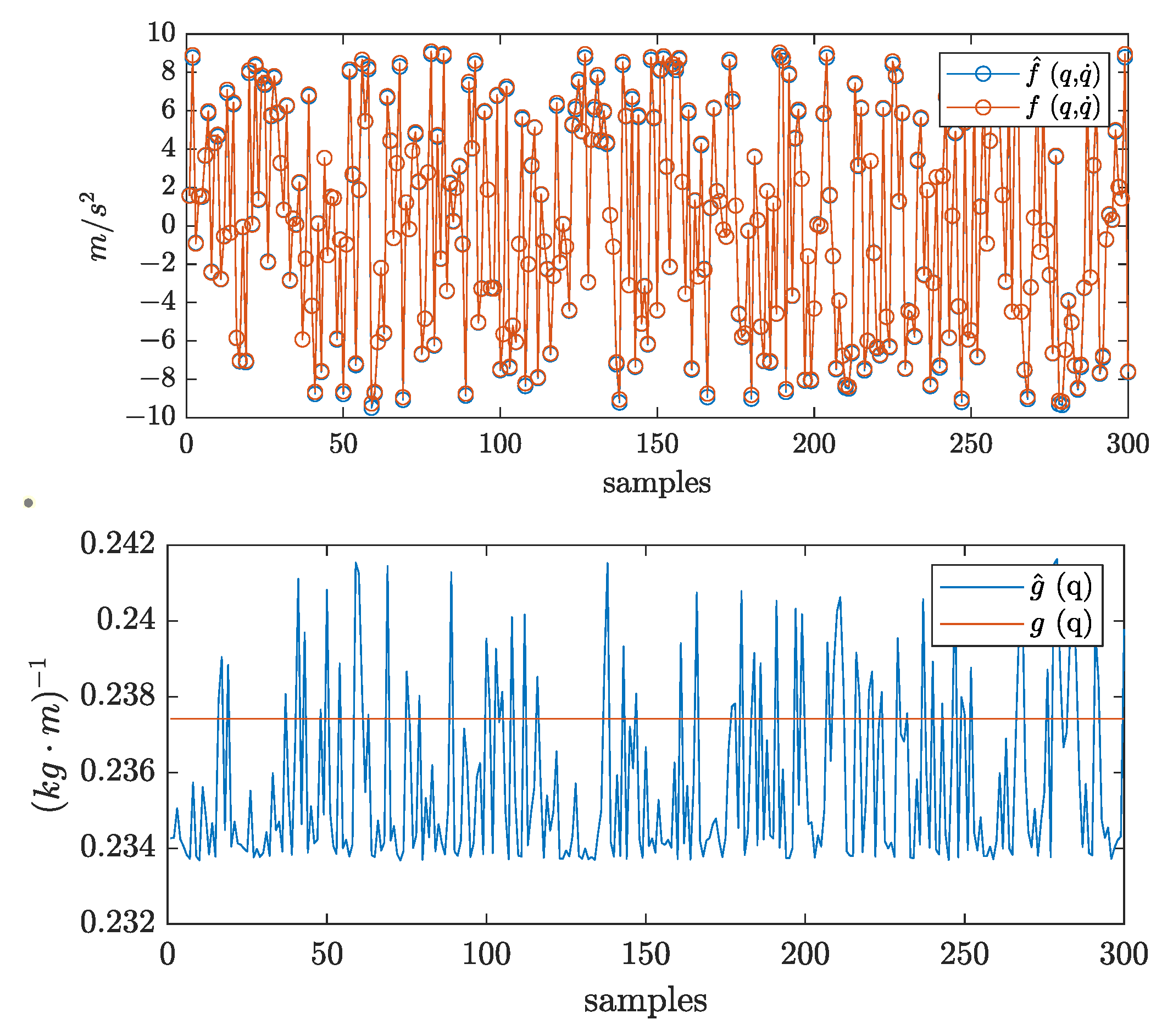
The neural network’s training was carried out for 20 iterations (i.e., 20 permutations of the overall 51 points in the workspace), so that the approximation improved sufficiently. The training of the adopted neural network structure over the collected data during each iteration (i.e., after each one of the 20 reference trajectories) was conducted using the MATLAB toolbox employing the default Levenberg–Marquardt algorithm. The results of the approximation problem can be observed in Figure 2 for the corresponding terms of f ( q , q ˙ ) and g ( q ) . It can be easily observed that through this process, we succeeded in obtaining a highly accurate (with an average relative approximation error less than 1 % ) estimate of the system dynamics, without relying on any prior knowledge.
In the second phase, we set a conventional PPC stabilizing controller, parametrized by k = 2 , λ = 2 , ρ 0 = π / 3 , ρ = π / 180 and l = 1.5 , as the initial admissible control policy. Our aim was to drive the system towards the fixed configuration q ¯ d = 0.5 , which is not a zero-input equilibrium of the system. The points used for the regression process were sampled from the set Ω q , ρ , ϵ = { 0 1 × ρ 10 ρ } × 0.45 0.45 } . Please note that the values chosen for the PPC controller, as well as the set adopted for the regression process should be specifically picked to take into consideration the desired prescribed performance specifications, as well as the system’s region of operation, respectively. For the integral cost, the weights α = 0.5 and β = 0.5 were chosen to specify an equal trade-off between the error convergence and the requested input energy. Moreover, P = 2500 points were chosen within Ω q , ρ , ϵ , and the number of constraints was set to M = 1250 . The cost function was approximated by 32 polynomial basis functions, chosen as follows: σ ( q , ρ , ϵ ) = T i 1 ( q ) T i 2 ( ε ) T i 3 ( ρ ) i 1 , i 2 = { 1 , , 4 } & i 3 = { 1 , 2 } , where T i ( · ) denotes the Chebyshev polynomial of degree i. An important property of these polynomials is that they are orthogonal with respect to the inner product, rendering them ideal for performing polynomial regression.
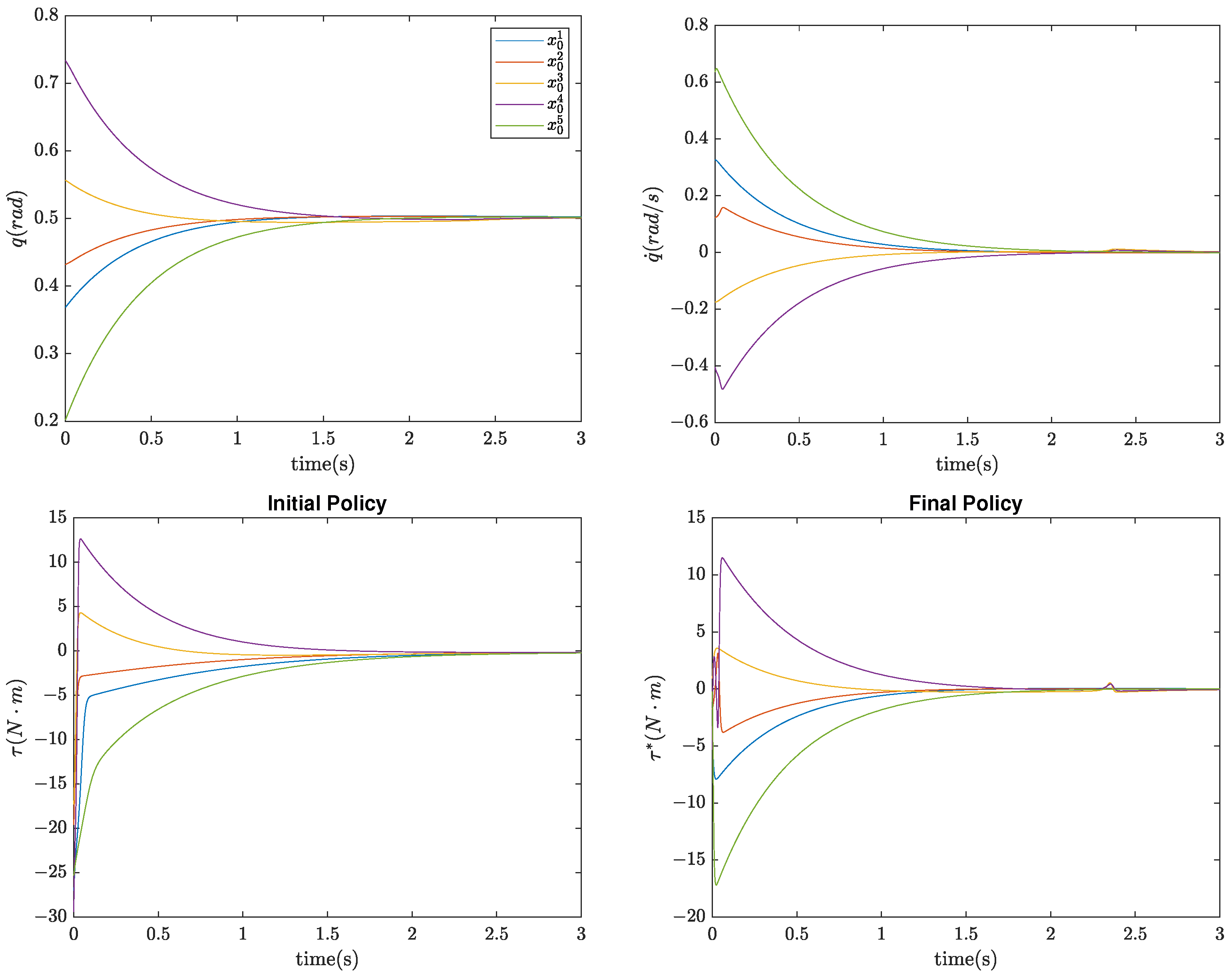
The response of the system under the optimal policy was simulated for 3 s for five different initial conditions and is illustrated in Figure 3, where the ability of the algorithm to stabilize the system under strict performance specifications is demonstrated. The initial conditions for these simulations are included in Table 1, along with a comparison between the costs of the initial admissible PPC policy, the final one, and an optimal control policy obtained through a successive approximation strategy similar to [30]. The response of the system under the new optimal policy was simulated for 3 s for the same initial conditions and is illustrated in Figure 4, along with the control effort requested by it. While it is clear that this policy results in significantly less control effort and thus a decrease in cost, note that this comes at the expense of sacrificing prescribed performance, as it is dictated by the parameters of the adopted performance function. This becomes evident in Figure 4, where it can be seen that for the initial conditions x 0 1 , the tracking error σ 1 ( t ) in our method stays within the region defined by the performance function, while the tracking error σ 2 ( t ) escapes the region, indicating the other policy’s trade-off of prescribed performance for optimality.
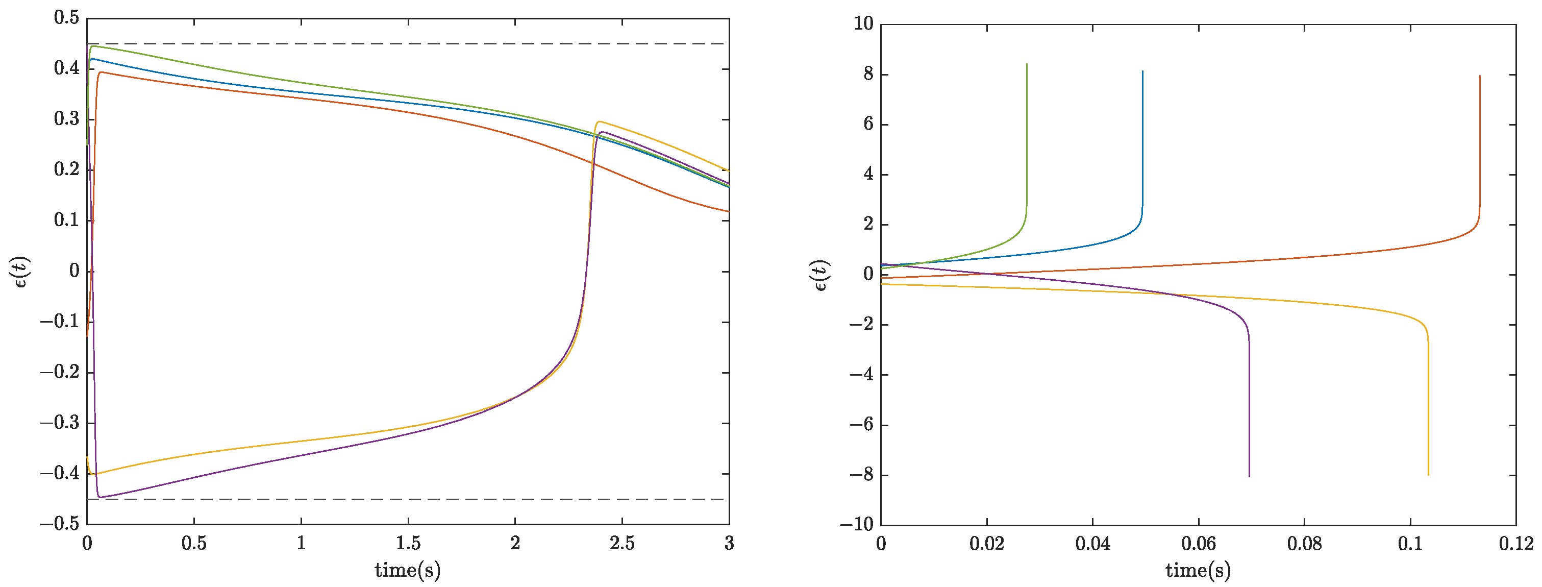
Regarding our method, it can be easily observed that the cost was successfully decreased, owing mainly to the reduction in the required control effort and despite the fact that we confined the system evolution within the set where the approximation capabilities of the polynomial structure held. Finally, Figure 5 shows the evolution of the transformed error. Notice that even though all initial conditions lie within Ω z , if we obtain the weights w L through the solution of the unconstrained least squares problem (17), the trajectories of ϵ escape the set Ω z , and τ * grows unbounded. However, by imposing a set of inequalities for w L as described in Section 4.2, the transformed error evolves strictly within Ω z , where the polynomial approximation holds, and thus optimality along with prescribed performance specifications are met.

5.2. Case B: 2-DOF Robotic Manipulator

In this section, we present simulation results that demonstrate the effectiveness of our methodology in deriving a near-optimal control law, while taking into consideration prescribed performance specifications, for a two-degree-of-freedom robotic manipulator, as illustrated in Figure 6. The robotic manipulator obeys the following dynamic model
M ( q ) q ¨ + C ( q , q ˙ ) q ˙ + G ( q ) = τ ,
where q = [ q 1 q 2 ] T and q ˙ = [ q ˙ 1 q ˙ 2 ] T denote the joint angular positions and velocities, respectively, M ( q ) is a positive definite inertia matrix, C ( q , q ˙ ) is the matrix that describes the Coriolis centrifugal phenomena, G ( q ) is the vector describing the influence of gravity, and τ is the torque that acts as the system’s input.
More specifically, the inertia matrix is formulated as:
M = M 11 M 12 M 21 M 22
where
M 11 = I Z 1 + I Z 2 + m 1 l 1 2 4 + m 2 ( l 1 2 + l 2 2 4 + l 1 l 2 c 2 ) M 12 = M 21 = I Z 2 + m 2 ( l 2 2 4 + 1 2 l 1 l 2 c 2 ) M 22 = I Z 2 + m 2 l 2 2 4
In addition, the vector containing the Coriolis and centrifugal torques is defined as follows:
C ( q , q ˙ ) q ˙ = c q 2 ˙ + k 1 c ( q 1 ˙ + q 2 ˙ ) c q 1 ˙ k 2 q 1 ˙ q 2 ˙
with c being c = 1 2 m 1 g l 1 l 2 s 2 . Additionally, the gravity vector is given by
G ( q ) = 1 2 m 1 g l 1 c 1 + m 2 g ( l 1 c 1 + 1 2 l 2 c 12 ) 1 2 m 2 l 2 g c 12
and the terms c 2 , s 2 and c 12 correspond to cos ( q 2 ) , sin ( q 2 ) and cos ( q 1 + q 2 ) , respectively. The values adopted for the simulation are depicted in Table 2, with m i , I z i and l i denoting the mass, the moment of inertia and the length of link i, respectively, k i being the joint friction coefficient and g the acceleration of gravity.
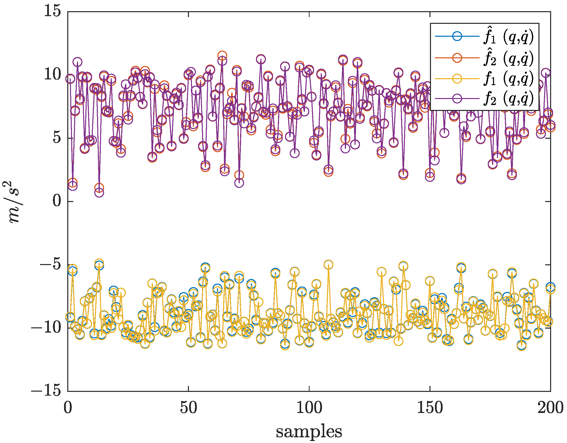
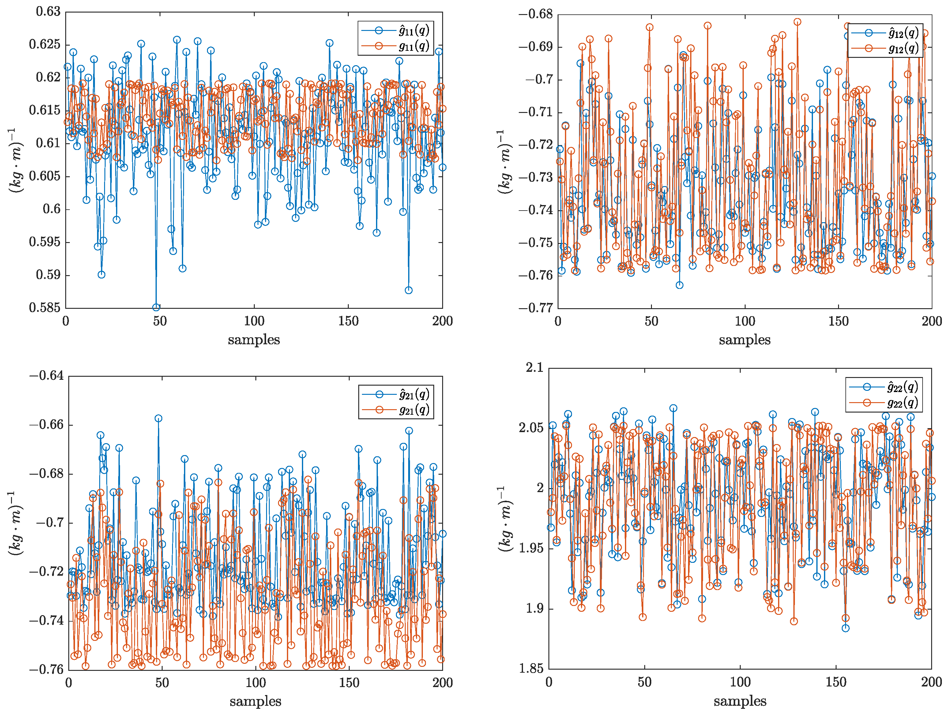
In order to retrieve the manipulator’s dynamics, a reference trajectory was designed so that it traversed (in random order) 71 points scattered over the compact set Ω q × Ω q ˙ = [ 1 , 1 ] × [ 1 , 1 ] × [ 1 , 1 ] × [ 1 , 1 ] . In order to track it, a PPC controller with gains k = 2 and λ = 7 was used, with performance specifications dictated by ρ 0 1 = π / 3 , ρ 1 = π / 180 , l 1 = 1.5 , ρ 0 2 = π / 3 , ρ 2 = π / 180 and l 2 = 1.5 . In addition, the gains of the tracking differentiator were chosen as k z 1 = k z 2 = 0.2 and R = 10 5 . For the system identification phase, a shallow neural network of one hidden layer containing 12 neurons was utilized to extract the system dynamics via the learning process, and the simulation was carried out for 20 iterations so that a sufficiently accurate approximation was obtained. The results of the identification problem are depicted in Figure 7 for the corresponding terms of f ( q , q ˙ ) = M 1 ( q ) ( C ( q , q ˙ ) q ˙ + G ( q ) ) and Figure 8 for the corresponding terms of g ( q ) = M 1 ( q ) .
In the second phase, we set a conventional PPC stabilizing controller, parametrized by k = 2 , λ = 2 , ρ 0 1 = ρ 0 2 = π / 3 , ρ 1 = ρ 2 = π / 180 and l 1 = l 2 = 1.5 , as the initial admissible control policy. Our aim was to drive the system towards the fixed configuration [ q ¯ 1 d , q ¯ 2 d ] T = [ π / 6 , π / 6 ] T . The points used for the regression process were sampled from the set:
Ω q , ρ , ϵ = { 0.5 0.5 × 0.45 0.45 × ρ 1 10 ρ 1 × 0.5 0.5 × 0.45 0.45 × ρ 2 10 ρ 2 }
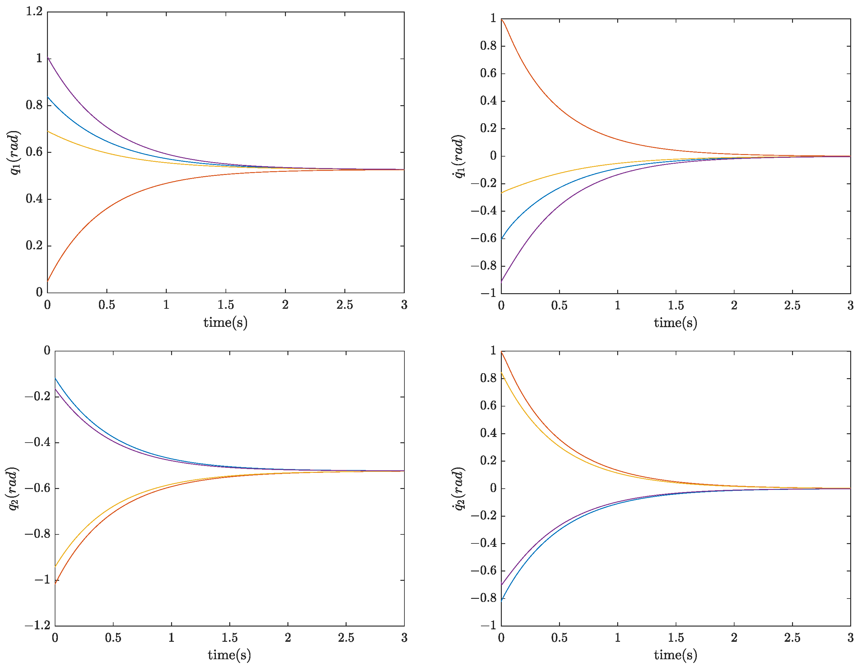
For the integral cost, the weights α = 0.5 and β = 0.5 were chosen to specify an equal trade-off between the error convergence and the requested input energy. Moreover, P = 8000 points were chosen within Ω q , ρ , ϵ , and the number of constraints was set to M = 1250 . The cost function was approximated by 64 polynomial basis functions, chosen as follows: σ ( q , ρ , ϵ ) = T i 1 ( q ) T i 2 ( ε ) T i 3 ( ρ ) i 1 , i 2 , i 3 = { 1 , , 2 } , where T i ( · ) denotes the Chebyshev polynomial of degree i. The response of the system under the optimal policy was simulated for 3 s for four different initial conditions and is illustrated in Figure 9 and Figure 10, where the ability of the algorithm to stabilize the system under strict performance specifications is demonstrated. The initial conditions for these simulations are included in Table 3, along with a comparison between the costs of the initial admissible policy and the final optimal one. It is evident that the cost was successfully decreased, owing mainly to the reduction in the required control effort.

6. Conclusions

A near-optimal control policy with a predefined transient and steady-state response for uncertain Euler–Lagrange dynamics was proposed. The method consisted of a neural network identifier, capable of accurately extracting the unknown dynamics as well as an iterative process for solving the HJB equation in order to produce an optimal stabilizing control policy with prescribed performance. The aforementioned approach was demonstrated through extensive simulation studies on a pendulum and a two-degree-of-freedom robotic manipulator. Future work will focus on expanding this method so that it is applicable to other classes of systems, while taking into consideration input and state constraints.

Author Contributions

Conceptualization, C.P.B. and K.J.K.; methodology, I.M. and C.P.B.; software, I.M. and C.V.; validation, I.M. and C.V.; formal analysis, I.M. and C.V.; investigation, all; resources, C.P.B.; data curation, I.M. and C.V.; writing—original draft preparation, I.M. and C.V.; writing—review and editing, C.P.B. and K.J.K.; visualization, C.V.; supervision, C.P.B. and K.J.K.; project administration, C.P.B.; funding acquisition, C.P.B. All authors have read and agreed to the published version of the manuscript.

Funding

The work of C.V. and C.P.B. was funded by the Hellenic Foundation for Research and Innovation (H.F.R.I.) under the second call for research projects to support postdoctoral researchers (HFRI-PD19-370).

Institutional Review Board Statement

Not applicable.

Informed Consent Statement

Not applicable.

Data Availability Statement

Data for this study are available from the corresponding author on request.

Conflicts of Interest

The authors declare no conflict of interest.

References

  1. Powell, W.B.; Ryzhov, I.O. Optimal Learning and Approximate Dynamic Programming. In Reinforcement Learning and Approximate Dynamic Programming for Feedback Control; John Wiley & Sons, Ltd.: Hoboken, NJ, USA, 2012; Chapter 18; pp. 410–431. [Google Scholar]
  2. Kirk, D. Optimal Control Theory: An Introduction; Dover Books on Electrical Engineering Series; Dover Publications: Mineola, NY, USA, 2004. [Google Scholar]
  3. Lewis, F.L.; Vrabie, D. Reinforcement learning and adaptive dynamic programming for feedback control. IEEE Circuits Syst. Mag. 2009, 9, 32–50. [Google Scholar] [CrossRef]
  4. Werbos, P. Elements of intelligence. Cybernetica 1968, 11, 131. [Google Scholar]
  5. Al-Tamimi, A.; Lewis, F.L.; Abu-Khalaf, M. Discrete-Time Nonlinear HJB Solution Using Approximate Dynamic Programming: Convergence Proof. IEEE Trans. Syst. Man Cybern. Part B Cybern. 2008, 38, 943–949. [Google Scholar] [CrossRef] [PubMed]
  6. Wang, F.Y.; Jin, N.; Liu, D.; Wei, Q. Adaptive Dynamic Programming for Finite-Horizon Optimal Control of Discrete-Time Nonlinear Systems with ε-Error Bound. IEEE Trans. Neural Netw. 2011, 22, 24–36. [Google Scholar] [CrossRef] [PubMed]
  7. Hornik, K.; Stinchcombe, M.; White, H. Multilayer feedforward networks are universal approximators. Neural Netw. 1989, 2, 359–366. [Google Scholar] [CrossRef]
  8. Jiang, Y.; Jiang, Z.P. Robust Adaptive Dynamic Programming and Feedback Stabilization of Nonlinear Systems. IEEE Trans. Neural Netw. Learn. Syst. 2014, 25, 882–893. [Google Scholar] [CrossRef] [PubMed]
  9. Zhao, B.; Liu, D.; Luo, C. Reinforcement Learning-Based Optimal Stabilization for Unknown Nonlinear Systems Subject to Inputs with Uncertain Constraints. IEEE Trans. Neural Netw. Learn. Syst. 2020, 31, 4330–4340. [Google Scholar] [CrossRef] [PubMed]
  10. Gao, W.; Jiang, Z.P. Learning-Based Adaptive Optimal Tracking Control of Strict-Feedback Nonlinear Systems. IEEE Trans. Neural Netw. Learn. Syst. 2018, 29, 2614–2624. [Google Scholar] [CrossRef] [PubMed]
  11. Jiang, Y.; Gao, W.; Na, J.; Zhang, D.; Hämäläinen, T.T.; Stojanovic, V.; Lewis, F.L. Value iteration and adaptive optimal output regulation with assured convergence rate. Control Eng. Pract. 2022, 121, 105042. [Google Scholar] [CrossRef]
  12. Chen, C.; Modares, H.; Xie, K.; Lewis, F.L.; Wan, Y.; Xie, S. Reinforcement Learning-Based Adaptive Optimal Exponential Tracking Control of Linear Systems with Unknown Dynamics. IEEE Trans. Autom. Control 2019, 64, 4423–4438. [Google Scholar] [CrossRef]
  13. Kamalapurkar, R.; Dinh, H.; Bhasin, S.; Dixon, W.E. Approximate optimal trajectory tracking for continuous-time nonlinear systems. Automatica 2015, 51, 40–48. [Google Scholar] [CrossRef]
  14. Na, J.; Lv, Y.; Wu, X.; Guo, Y.; Chen, Q. Approximate optimal tracking control for continuous-time unknown nonlinear systems. In Proceedings of the 33rd Chinese Control Conference, Nanjing, China, 28–30 July 2014; pp. 8990–8995. [Google Scholar] [CrossRef]
  15. Na, J.; Lv, Y.; Zhang, K.; Zhao, J. Adaptive Identifier-Critic-Based Optimal Tracking Control for Nonlinear Systems with Experimental Validation. IEEE Trans. Syst. Man Cybern. Syst. 2022, 52, 459–472. [Google Scholar] [CrossRef]
  16. Zhao, K.; Song, Y.; Ma, T.; He, L. Prescribed Performance Control of Uncertain Euler–Lagrange Systems Subject to Full-State Constraints. IEEE Trans. Neural Netw. Learn. Syst. 2018, 29, 3478–3489. [Google Scholar] [CrossRef]
  17. Bhasin, S.; Kamalapurkar, R.; Johnson, M.; Vamvoudakis, K.; Lewis, F.; Dixon, W. A novel actor–critic–identifier architecture for approximate optimal control of uncertain nonlinear systems. Automatica 2013, 49, 82–92. [Google Scholar] [CrossRef]
  18. Bechlioulis, C.P.; Rovithakis, G.A. Robust Adaptive Control of Feedback Linearizable MIMO Nonlinear Systems with Prescribed Performance. IEEE Trans. Autom. Control 2008, 53, 2090–2099. [Google Scholar] [CrossRef]
  19. Yin, Z.; Luo, J.; Wei, C. Robust prescribed performance control for Euler–Lagrange systems with practically finite-time stability. Eur. J. Control 2020, 52, 1–10. [Google Scholar] [CrossRef]
  20. Jabbari Asl, H.; Narikiyo, T.; Kawanishi, M. Bounded-input prescribed performance control of uncertain Euler–Lagrange systems. IET Control Theory Appl. 2019, 13, 17–26. [Google Scholar] [CrossRef]
  21. Dong, H.; Zhao, X.; Luo, B. Optimal Tracking Control for Uncertain Nonlinear Systems with Prescribed Performance via Critic-Only ADP. IEEE Trans. Syst. Man Cybern. Syst. 2022, 52, 561–573. [Google Scholar] [CrossRef]
  22. Fortuna, L.; Frasca, M. Optimal and Robust Control: Advanced Topics with MATLAB®; CRC Press: Boca Raton, FL, USA, 2012. [Google Scholar] [CrossRef]
  23. Dimanidis, I.S.; Bechlioulis, C.P.; Rovithakis, G.A. Output Feedback Approximation-Free Prescribed Performance Tracking Control for Uncertain MIMO Nonlinear Systems. IEEE Trans. Autom. Control 2020, 65, 5058–5069. [Google Scholar] [CrossRef]
  24. Kosmatopoulos, E.B.; Ioannou, P.A. Robust switching adaptive control of multi-input nonlinear systems. IEEE Trans. Autom. Control 2002, 47, 610–624. [Google Scholar] [CrossRef]
  25. Bechlioulis, C.P.; Rovithakis, G.A. Prescribed Performance Adaptive Control for Multi-Input Multi-Output Affine in the Control Nonlinear Systems. IEEE Trans. Autom. Control 2010, 55, 1220–1226. [Google Scholar] [CrossRef]
  26. Lewis, F.L.; Vrabie, D.L.; Syrmos, V.L. Optimal Control; John Wiley & Sons, Inc.: Hoboken, NJ, USA, 2012. [Google Scholar] [CrossRef]
  27. Guo, B.Z.; Zhao, Z. On convergence of tracking differentiator. Int. J. Control 2011, 84, 693–701. [Google Scholar] [CrossRef]
  28. Rousseas, P.; Bechlioulis, C.; Kyriakopoulos, K.J. Harmonic-Based Optimal Motion Planning in Constrained Workspaces Using Reinforcement Learning. IEEE Robot. Autom. Lett. 2021, 6, 2005–2011. [Google Scholar] [CrossRef]
  29. Potra, F.A.; Wright, S.J. Interior-point methods. J. Comput. Appl. Math. 2000, 124, 281–302. [Google Scholar] [CrossRef]
  30. Abu-Khalaf, M.; Lewis, F.L. Nearly optimal control laws for nonlinear systems with saturating actuators using a neural network HJB approach. Automatica 2005, 41, 779–791. [Google Scholar] [CrossRef]
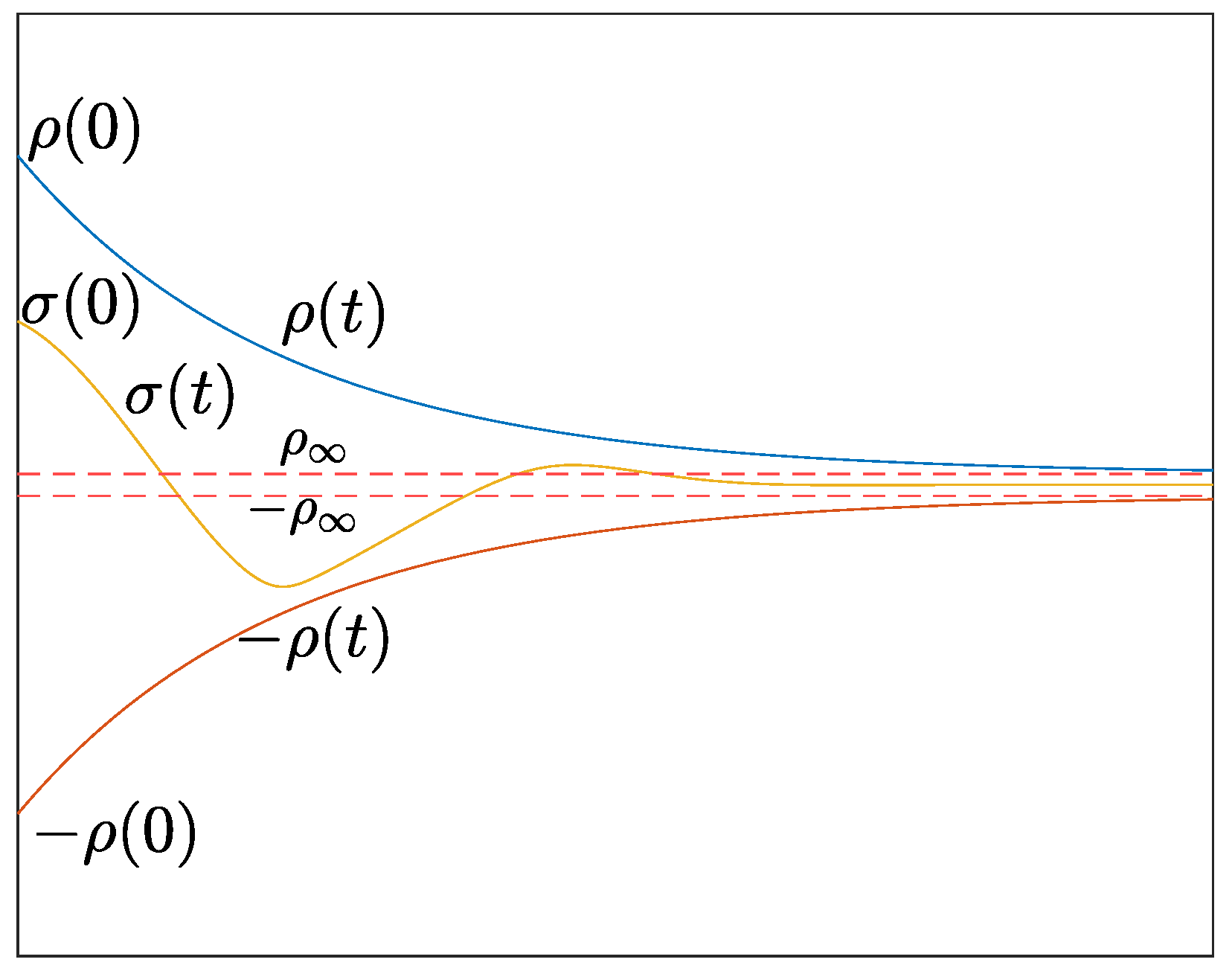
Figure 1. Graphical representation of (3).
Applsci 13 11923 g001
Figure 2. Comparison between the actual values and their estimates for f ( q , q ˙ ) (top) and g ( q ) (bottom) for 300 random samples within Ω q × Ω q ˙ .
Applsci 13 11923 g002
Figure 3. The state response of the calculated optimal PPC scheme (top). Comparison between the control effort τ G ( q d ) requested by the initial and the optimal PPC policies (bottom).
Applsci 13 11923 g003
Figure 4. The state response of the calculated optimal scheme (top). Control effort τ G ( q d ) requested by the optimal policy (bottom left). Comparison of the tracking error’s evolution for the initial condition x 0 1 between our method ( σ 1 ) and successive approximation ( σ 2 ) (bottom right).
Applsci 13 11923 g004
Figure 5. Evolution of the transformed error ϵ by utilizing w L obtained from the constrained (left) and the unconstrained (right) least-squares problem. The dashed lines represent the values of ϵ on the boundary of Ω z .
Applsci 13 11923 g005
Figure 6. Two-DOF robotic manipulator.
Applsci 13 11923 g006
Figure 7. Comparison between the actual values and their estimates for f 1 ( q , q ˙ ) (bottom) and f 2 ( q , q ˙ ) (top) for 200 random samples within Ω q × Ω q ˙ .
Applsci 13 11923 g007
Figure 8. Comparison between the actual values and their estimates for g 11 ( q ) , g 12 ( q ) , g 21 ( q ) and g 22 ( q ) for 200 random samples within Ω q × Ω q ˙ . .
Applsci 13 11923 g008
Figure 9. The state response of the calculated optimal PPC scheme for various initial conditions.
Applsci 13 11923 g009
Figure 10. Comparison between the control effort τ G ( q d ) requested by the initial and the optimal PPC policies.
Applsci 13 11923 g010
Table 1. Comparison between the initial PPC policy and the final optimal one.
Initial Condition
[ q ( 0 ) , ρ ( 0 ) , ϵ ( 0 ) ]
Initial Policy’s CostFinal Policy’s CostFinal Policy’s Cost (Without Prescribed Performance)
[ 0.73 , 0.148 , 0.45 ] 22.60 16.79 0.47
[ 0.2 , 0.165 , 0.25 ] 45.54 34.83 1.01
[ 0.56 , 0.174 , 0.37 ] 3.21 1.59 0.05
[ 0.37 , 0.173 , 0.37 ] 6.63 1.4 0.21
[ 0.43 , 0.11 , 0.13 ] 3.90 1.80 0.05
Table 2. Two-DOF robotic manipulator parameter values.
m 1  (kg) l 1  (m) I Z 1 ( kg · m 2 ) k 1  (kg/s) m 2  (kg) l 2  (m) I Z 2 ( kg · m 2 ) k 2  (kg/s) g ( m / s 2 )
3.20.50.9612.00.40.8119.81
Table 3. Comparison between the initial PPC policy and the final optimal one.
Initial Condition
[ q 1 ( 0 ) , ρ 1 ( 0 ) , ϵ 1 ( 0 ) ] ,
[ q 2 ( 0 ) , ρ 2 ( 0 ) , ϵ 2 ( 0 ) ]
Initial Policy’s CostFinal Policy’s Cost
[ 0.84 , 0.17 , 0.159 ] , [ 0.12 , 0.108 , 0.11 ] 5.24 1.18
[ 0.05 , 0.145 , 0.29 ] , [ 1.02 , 0.106 , 0.134 ] 7.24 4.16
[ 0.69 , 0.171 , 0.425 ] , [ 0.94 , 0.101 , 0.09 ] 5.69 1.01
[ 1.01 , 0.118 , 0.42 ] , [ 0.165 , 0.149 , 0.27 ] 5.66 1.39
Disclaimer/Publisher’s Note: The statements, opinions and data contained in all publications are solely those of the individual author(s) and contributor(s) and not of MDPI and/or the editor(s). MDPI and/or the editor(s) disclaim responsibility for any injury to people or property resulting from any ideas, methods, instructions or products referred to in the content.