Abstract
The approach advanced by Harrison puts in the spotlight the fundamental role of bistability in hysteresis modeling. The description is based on physical premises concerning irreversible thermodynamics. In the original model, the upscaling of irreversible phenomena acting on the micromagnetic level is carried out by the introduction of a phenomenological parameter β. In the present paper, an alternative approach is proposed. The outputs of individual outputs of elementary hysteresis units (hysterons) are considered like in the stop model. A verification of the proposed model is carried out using measurement data for a praseodymium–dysprosium ribbon sample and a cylinder core made of cobalt-based amorphous material.
1. Introduction
Hysteresis modeling is important for practitioners dealing with descriptions of magnetic properties of materials readily used in Nondestructive Testing and Evaluation. This topic is also in the spotlight of MDPI’s Applied Sciences journal, just to mention recent publications [1,2]. As was pointed out in [1,3], the hysteresis phenomenon is prevalent in different areas of science, yet its occurrence in ferromagnetic materials remains a paradigm [4].
The present contribution is inspired by an excellent review work published recently [5]. It extends several concepts which have been mentioned in the previous publications [6,7,8,9]. The fundamental concept of the paper is to modify the Harrison model of ferromagnetism to make it more useful for engineering purposes. The modification relies on the summation of responses of elementary bistable units operating on the quantum level using an approach like the stop models.
The original description advanced twenty years ago [10] may be perceived as a “toy model” because of its spurious simplicity. However, it is based on a profound physical interpretation; moreover, it is consistent with the laws of irreversible thermodynamics. It distinguishes the reversible and irreversible magnetization processes and offers a simple interpretation of the hysteresis loop onset as related to quantum-mechanical effects.
The irreversible magnetization processes are expressed in dimensionless units with the following relationship as:
in which m stands for reduced magnetization, and h is reduced applied field strength, whereas t denotes temperature, referring to the Curie temperature. This self-consistent relationship (since reduced magnetization m appears on both sides of Equation (1)) puts in the central perspective the concept of the “effective” field, which is the true internal field acting on magnetic moments within the ferromagnetic substance. It is different from the externally applied field. In physical units, this concept may be written as:
where the dimensionless coefficient controlling the strength of interaction forces (referred to as the molecular field constant) is due to Weiss [11]. For a friendly introduction to the Weiss concept, the Readers are referred, e.g., to the textbooks [12,13], or, e.g., to [14]. The theory of effective field has been used to explain spontaneous magnetic ordering and phase transitions in ferromagnets [3], and it is widely used in solid-state physics; some widely used hysteresis models such as the Jiles–Atherton formalism [15] heavily explore and rely on the concept. It is, however, interesting to mention that the idea of mutual interactions between individual entities has influenced seemingly different research studies, e.g., those devoted to collective behavior [16,17] or focused on applied mathematics and computer science [18,19,20]. In the context of research on Nondestructive Testing and Evaluation, it should be stressed that the expression for the effective field may include additional terms related, e.g., to eddy currents, thermal viscosity, mechanical stresses or demagnetization effects [21], which opens an exciting perspective to develop new types of sensors of physical quantities based on monitoring of magnetic properties.
2. A Brief Introduction to the Harrison Model
In the original Harrison model, the Weiss’ mean field constant is assumed to be positive, just like in, e.g., the Jiles–Atherton approach—this corresponds to the positive feedback in the system. The argument of hyperbolic tangent in Equation (1) is written as the weighed sum . In that case, the curve given with Equation (1) is S shaped (if one considers dependence) or N shaped (if one considers dependence). It passes through the second and the fourth quadrants of the plane; the extreme points are referred to as bifurcation points.
Equation (1) may be easily inverted analytically; the description having magnetization as its input and field strength as its output is referred to as an inverse hysteresis model. The appropriate expression becomes:
where the reduced temperature plays the role of a weighting parameter.
The curve given with Equation (3) for a positive , , has two extreme points whose coordinates are computed from equating to zero. The fragment of the curve between these extreme points is decreasing; in ferroelectric devices, this corresponds to the “negative capacitance” effect, which recently has been the subject of intensive research [22,23] because of its potential applications, e.g., in low-power nanoscale devices. In ferromagnetic materials, in most cases, aside from in precise experiments carried out for single iron crystals [24], the intermediate region is hard to observe experimentally.
As field strength reaches the threshold value equal to , an abrupt jump to another hysteresis loop branch occurs. The magnetization value at which both branches coincide cannot be given in an analytical form; however, it is straightforward to compute it numerically.
Two extreme cases are:
- when the curvature of the function disappears. Then, the dependence is represented by a zigzag resembling the letter “N”. The value of field strength at the bifurcation point (considered equivalent to coercivity) reaches unity;
- when the hysteresis loop disappears.
In the original model, Harrison used a phenomenological parameter , which was introduced to scale the irreversible hysteresis curves operating on the micromagnetic level up to the domain size (mesoscopic) level, on which the anhysteretic processes occurred. The afore-given statement is clear if one considers the expression (1) written not in relative units but physical ones. It reads [10]:
where H/m is free space permeability, = 9.27 Am2 is the Bohr magneton, J/K is Boltzmann’s constant and dimensionless is Weiss’ mean field parameter (cf. (2)), whereas measured in K is the absolute temperature. stands for saturation magnetization. From the inspection of the above-given relationship, all quantities have a clear physical interpretation, whereas is merely a numerical means to scale the switching phenomenon, occurring at quantum scale up to the scale of magnetic domains. Harrison explained his approach in this way: “ … the new vector quantity can be called a “supermagneton”. In this model the “supermagneton” is a new quantum particle, that is acted upon by the effective field” [6].
In other words, the original approach corresponds to the multiplication effect for a single hysteresis operator; thus, it means that the model is subject to averaging and homogenization, not just because of the presence of the averaged quantity but also because all operators are treated as the same. According to the model developer, the Weiss coefficient accounts for the exchange field between atomic moments, while the domain coefficient, i.e., , describes the atomic moment summation process [6].
The outcome of hysteresis loops with realistic shapes were obtained by summing field strength contributions corresponding to the irreversible and reversible re-magnetization processes, cf. [10] or Figure 3 in [8]. The concept of the present paper is to introduce a weighted summation from several elementary irreversible hysteresis operators and, thus, to treat the elementary Harrison unit as a generalized stop operator [5,25,26]. In this context, the idea behind the present paper corresponds to the one outlined in recent publication [27], in which, however, the hysteretic characteristics of elementary units are assumed to be composed of broken line segments. The proposed approach considered in the present paper allows one to obtain better flexibility and fitting accuracy.
It should be emphasized that there exists a profound connection between the Harrison approach and theory of phase transitions advanced by Landau [28]. A refinement of the Landau theory, known as the Landau–Ginsburg–Devonshire approach, plays a crucial role in the understanding of the basic physics of ferroelectricity [14,23].
2.1. An Alternative Elementary Unit (“Hysteron”)
As pointed out earlier, the reduced field strength modeled with the original Harrison description rarely reaches values close to zero; for example, for Fe–Si electrical steels, the maximal value is around 0.498 [8] since the reduced temperature [10]. Our goal was to find out a functional dependence which would behave qualitatively like the one given with (3) yet able to reach within the bounds For such a functional relationship, it might be easier to assign weights to individual units and interpret the results. Inspired by the work [29], which stressed the flexibility of logistic mapping and its usefulness in phenomenological descriptions of ferromagnetic hysteresis, we considered the following relationship for the description of the double-well energy landscape in an elementary hysteretic unit as:
where is a constant.
Following the monograph [3], we considered a connection between hysteresis phenomenon and metastability. The proper framework for examination of this relationship is thermodynamics of irreversible phenomena. If we consider a system with local memory, just three variables, H, X (Bertotti’s notation, cf. chapter 2.1.4, here identified as M) and T, provide a complete characterization of states. If H and X are conjugate work variables, then G(H, T) = F (X, T) − H X is the corresponding Gibbs energy (F denotes the Helmholtz free energy of the system). To consider an energy profile with at least two minima symmetrically set with respect to the X axis, we need a polynomial of the order four.
Imposing the condition for the equilibrium of competing thermodynamic forces [3], we can write:
Thus, the dependence of the applied field versus magnetization becomes a polynomial of one order lower, i.e., of the order three. Let us notice that, due to symmetry, this polynomial has just odd order terms. Of course, it is possible to consider higher-order polynomials, which may possess local global minima, yet, in that case, the polynomials will also possess only odd terms.
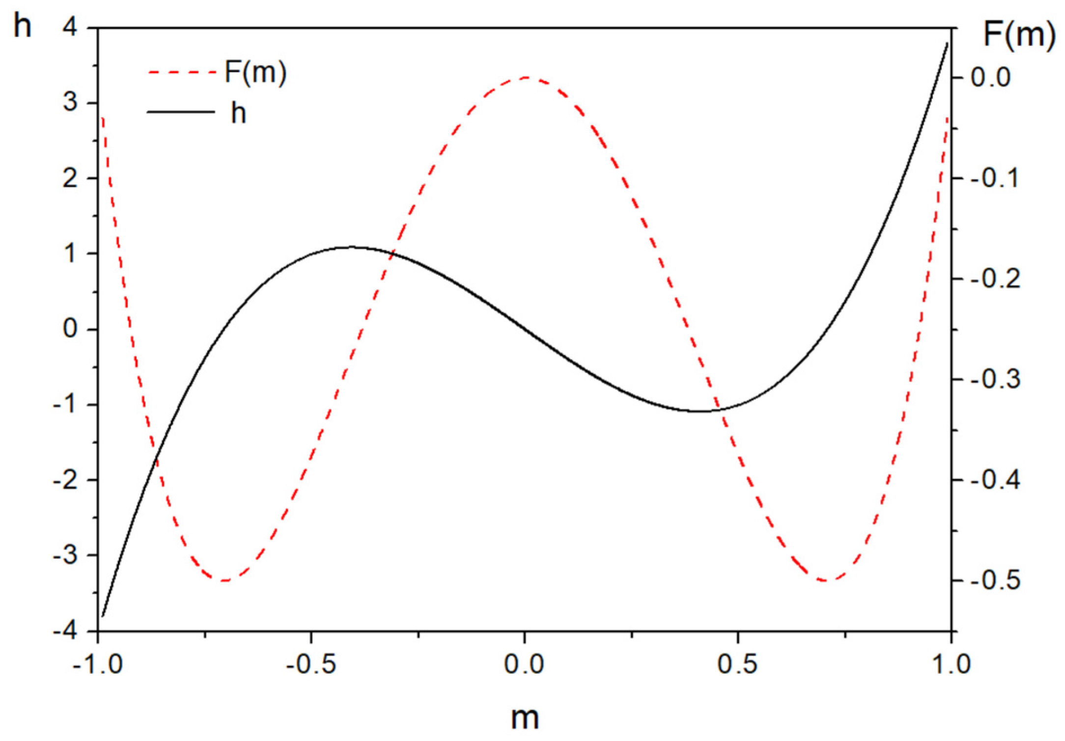
Figure 1 depicts the dependencies and for an arbitrary value
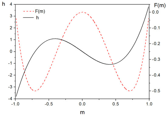
Figure 1.
The dependencies (broken line) and (solid line) for .
It is interesting to remark that the specific choice of (4) imposes several invariable values for some loop parameters such as remanence or regardless of the value. It can be proven that the choice allows one to obtain . A fixed remanence value might be considered a limitation since (4) is most appropriate for those materials for which the squareness of hysteresis loops (the ratio of remanence magnetization to saturation magnetization) [30] is close to 0.7. However, we would like to remark that alternative formulations for the dependence may also be applied. For example, a polynomial with odd powers is:
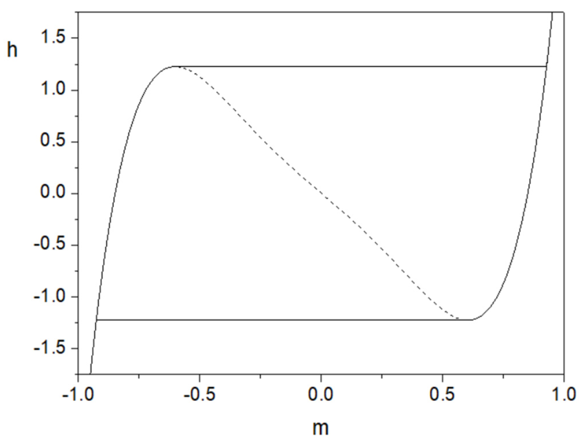
where the subscript denotes that powers with non-zero values of coefficients also behave qualitatively in a similar way. The relationship (6) is depicted in Figure 2. The remanence values for this polynomial are , and the bifurcation magnetization , whereas the corresponding value of field strength (coercive field strength) The value of magnetization when two branches of hysteresis loop coincide is approximately
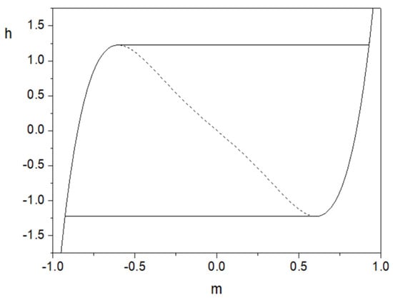
Figure 2.
The dependence and corresponding irreversible hysteresis loop.
A thorough examination in which combinations of coefficients for polynomials with odd powers yield qualitatively similar loops is beyond the scope of the present paper and is postponed to another publication. However, we would like to point out that the possibility to use different elementary units as building blocks for the generalized stop operator together with appropriate weighting allows one to obtain a certain level of flexibility for the description, which shall be shown in the subsequent part of this section.
2.2. The Effect from the Use of Different Elementary Units and Different Weights
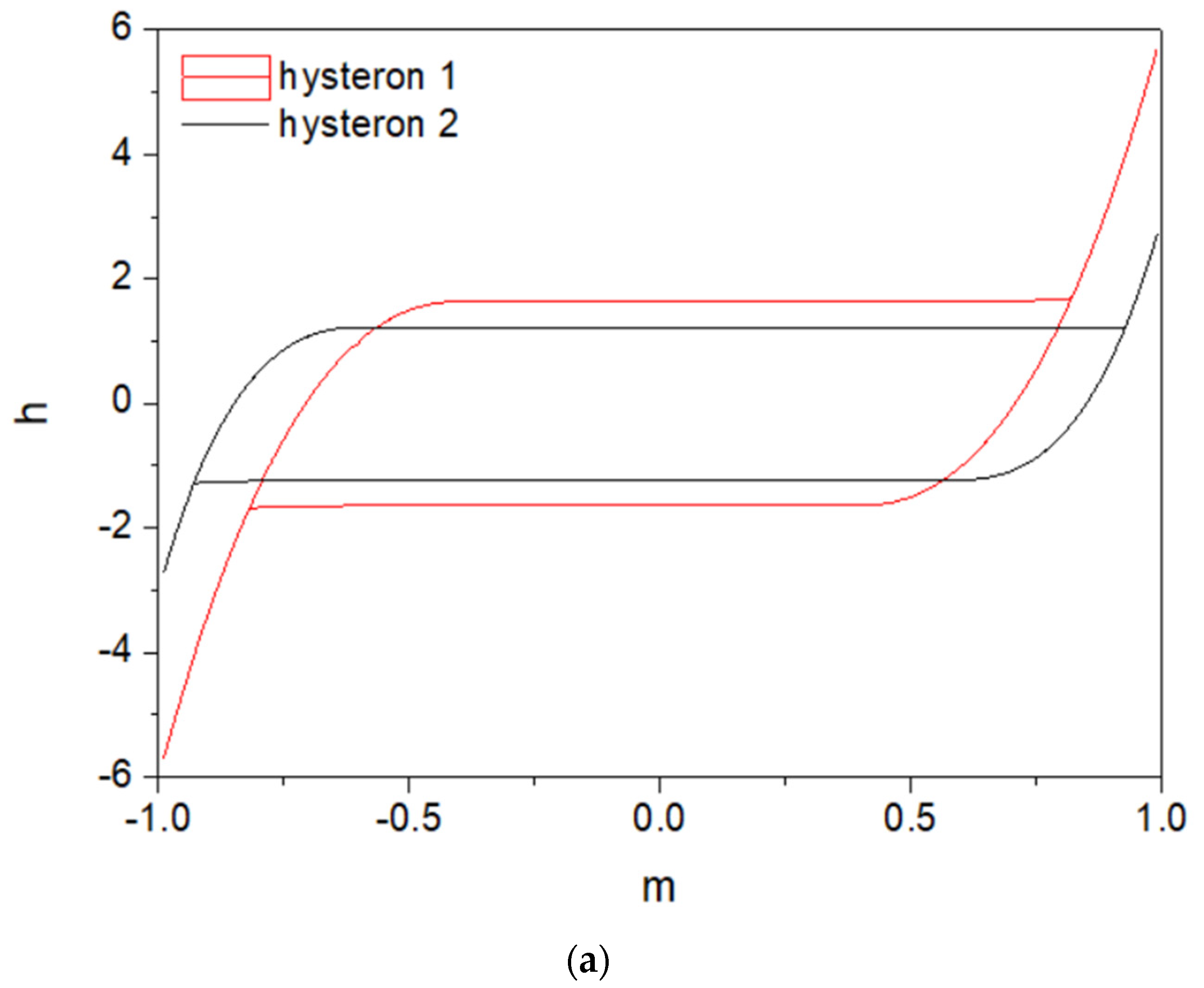
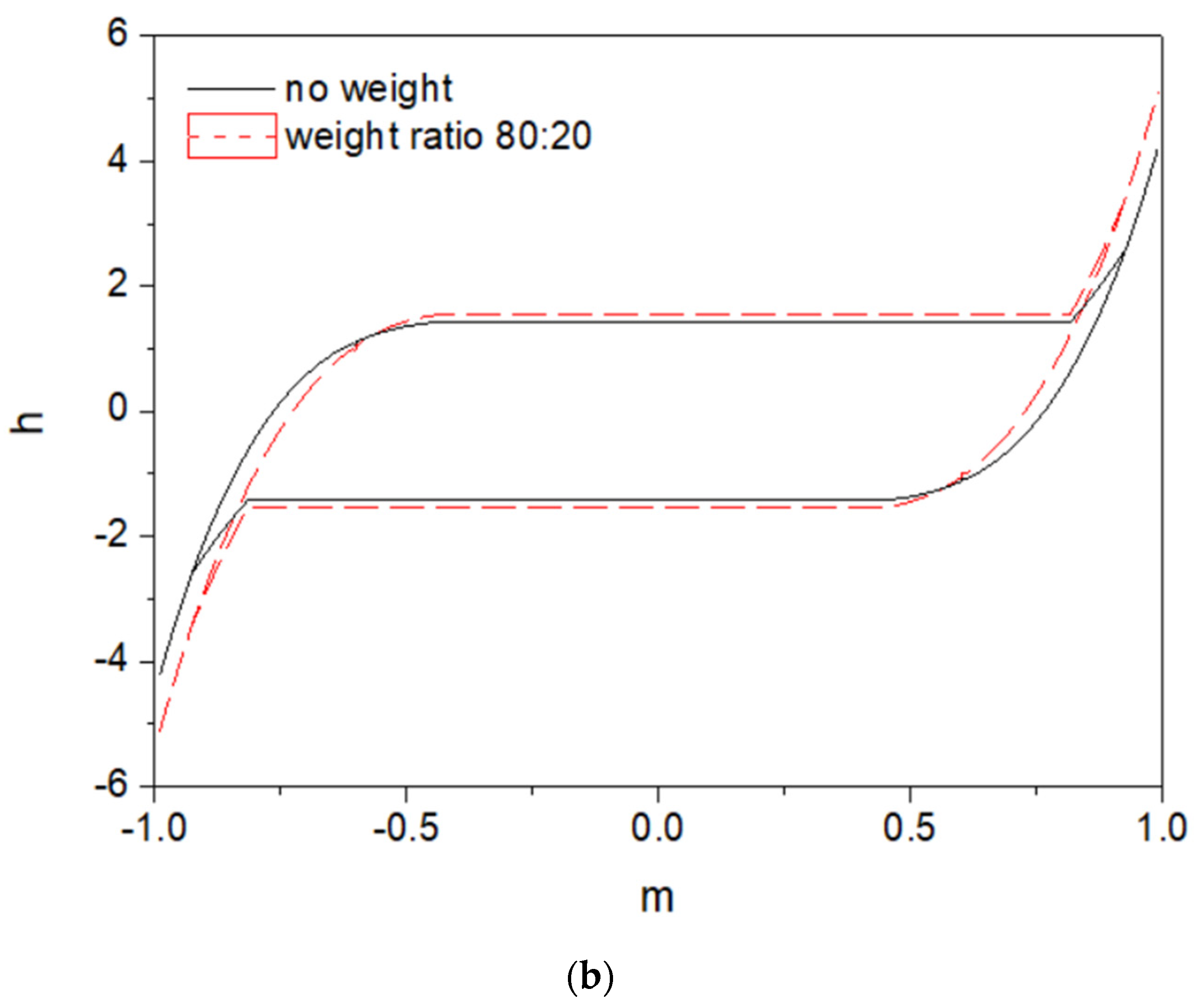
During preliminary tests, we simulated the effect of just two elementary units, one given with (5), where the value is set to , and the other given with (7). For the first unit, the loop coordinates at bifurcation points are and . Figure 3a depicts the component hysteresis loops, whereas Figure 3b shows the outcome loop for the case when no weighting was assumed, and thus the ratio of contributions was 50:50 (solid black line), and for the case when the weights were assigned following the ratio 80:20 (red dashed line).
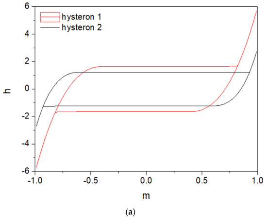
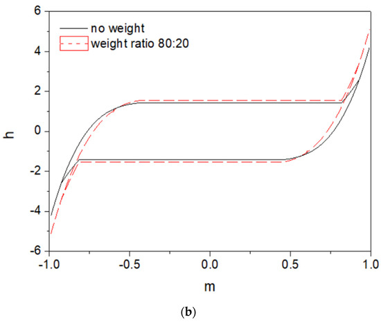
Figure 3.
The component loops (a) and corresponding outcome loops (b).
2.3. The Effect from Treating the “a” Parameter as a Random Variable
By analogy to the Preisach formalism in which different “hysterons” are assigned different coercive field strengths, and thus it is natural to work with their distributions, we assume that it is possible to treat the “” parameter in (6) as a random variable and to monitor the effect of the varying number of hysterons and their variance on the shape of the outcome hysteresis loops. In this context, our analysis is like the one presented in [31].
There is a direct correspondence between the values of parameter “” and coercive field strength for hysterons whose dependence is given with (6), namely,
Therefore, producing a distribution of the “” parameter with the mean value is equivalent to the introduction of hysteron distribution with coercive fields around unity.
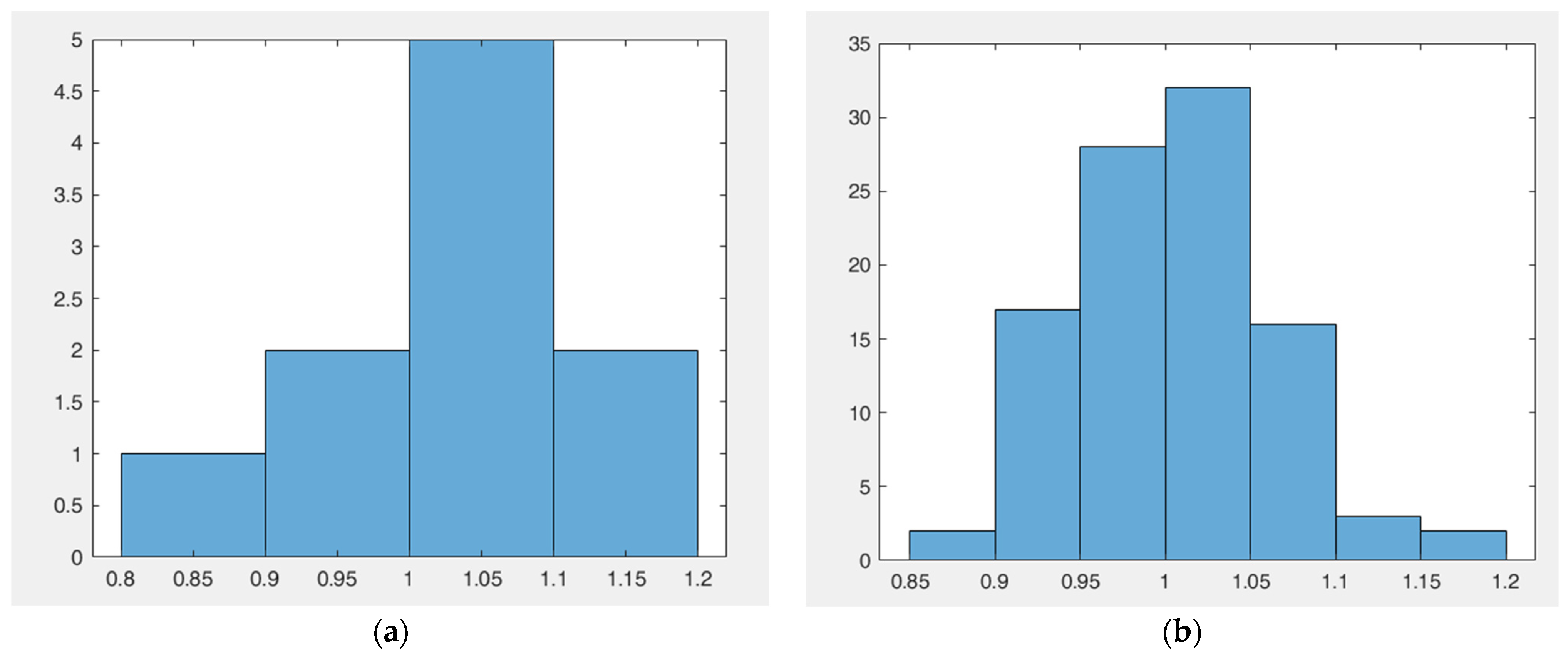
Figure 4 depicts the effect of increasing the number of hysterons. The mean value of coercive field strength is set to unity, the variance is set to 0.05. The seed of pseudo-random is in each case set to the same initial state (the appropriate MATLAB command is rng(‘default’)); thus, the sequences of pseudo-random numbers drawn from the normal distribution have the same initial components. We consider the cases when there are ten hysterons; next, we increase their number to one hundred. It can be noticed that an increase in number of hysterons makes their distribution look more like the Gaussian distribution, which can be appreciated from a visual comparison of obtained histograms. On the other hand, the computations of the outcome characteristic become more cumbersome as the number of hysterons is excessively high. It is beyond the scope of the present paper to present an identification method which will enable one to resolve how many individual hysterons should be taken into account and how to assign weights to their outputs; however, we think that artificial neural networks (ANNs) might be useful for the purpose since the very principle of superposition of stop operators resembles to a large extent the architecture of classical feed-forward ANNs.

Figure 4.
The histograms obtained (a) for ten and (b) for one hundred hysterons with mean value of coercive field set to unity and variance set to 0.05.
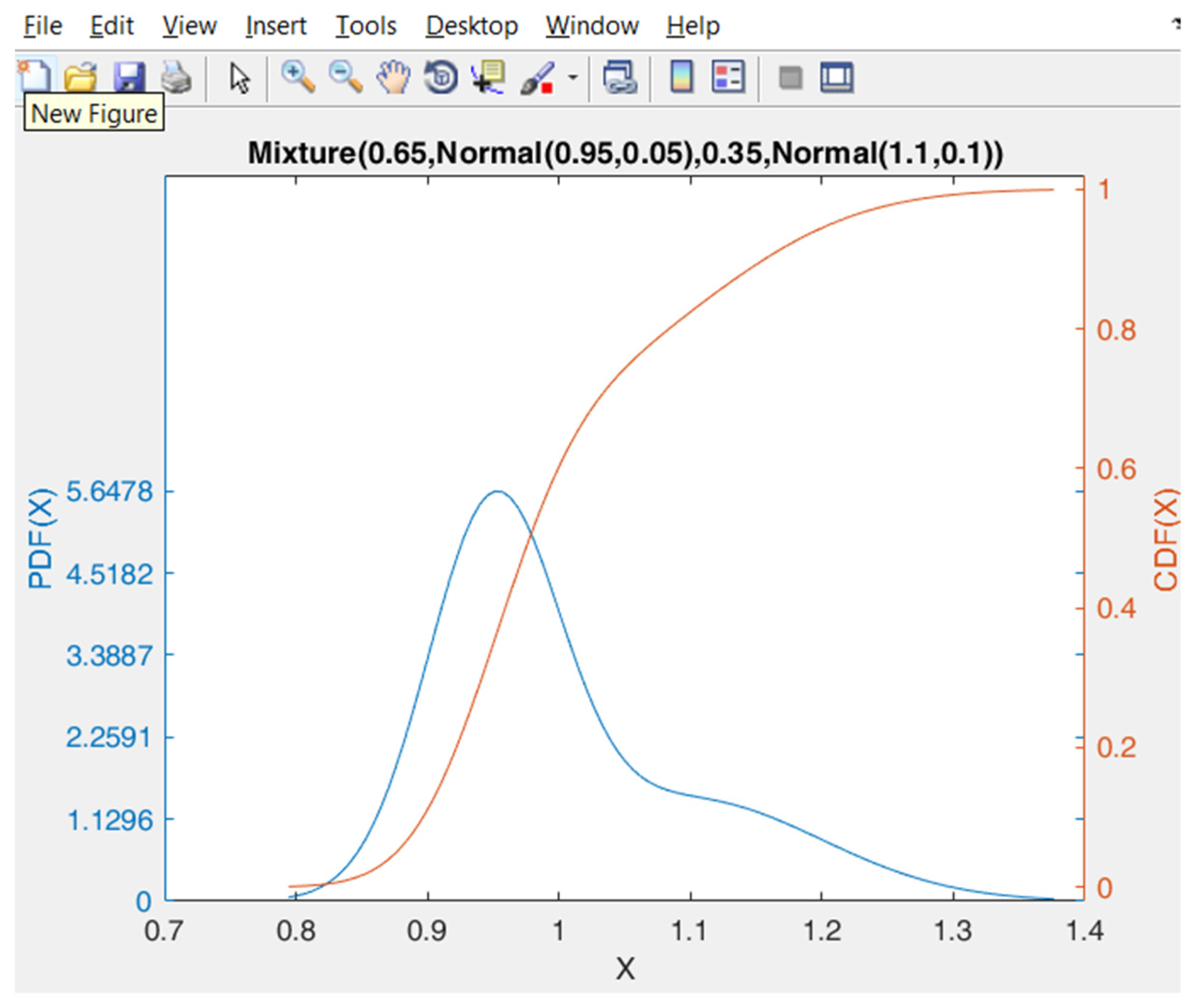
An additional refinement to the presented approach might be based on the use of the Gaussian Mixture model for several hysteron distributions differing in mean values and variances or, e.g., some other type of kernel (Epanechnikov, triangular). In the first case mentioned, we think that the MATLAB toolbox Cupid [32] might be useful. Figure 5 depicts the probability density function (PDF) and the cumulative density function (CDF) for a mixture of two normal distributions with different mean values, variances and weights. The plot was obtained using the commands:
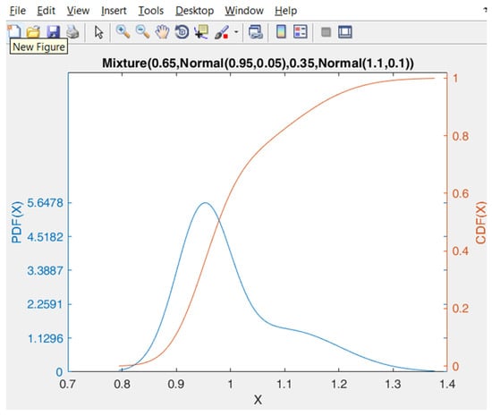
Figure 5.
The PDF and the CDF for a mixture of two distributions.
- myDist = Mixture(0.65, Normal(0.95, 0.05), 0.35, Normal(1.1, 0.1))
- myDist.PlotDens
The basic statistics on the mixed distribution are obtained by typing: [myDist.Mean, myDist.SD], which, in our example, yields ans = 1.0025 0.1012.
2.4. The Reversibility Effect
An advantage of the original Harrison model is that this description considers not just purely irreversible effects but also it explicitly speaks of reversibility, expressed with the anhysteretic curve. As already discussed in [9], there exists a discrepancy between this approach and the Jiles–Atherton (JA) formalism as far as the physical meaning of irreversible and reversible magnetization processes is concerned. Jiles and Atherton used the so-called effective field, being the sum of the applied field and the bulk magnetization multiplied by a positive constant α (by analogy to the Weiss mean field), as the argument of the function, which was supposed to describe the anhysteretic curve. Zirka et al. criticized the physical assumptions underlying the Jiles–Atherton description, indicating that the summation of irreversible and reversible magnetization components postulated by the model developers leads to the non-physical behavior of modeled curves after field reversals, which is to some extent patched using pseudo-parameter , whose role is to suppress the negative dynamic susceptibility regions [33]. However, the presence of cannot be justified from the derivation of model equations. The source of problems with the physical interpretation of the JA description is the fundamental assumption that the hysteresis loop is obtained by introducing offsets (shifts) from the “anhysteretic” curve along the (and not along the ) direction. A counter-example of the correct approach in the irreversible thermodynamics framework is the GRUCAD model [34], also studied by some of the authors of the present contribution [35]. The Harrison model bears a striking resemblance to the GRUCAD model in the sense that it distinguishes irreversible and reversible contributions as field strength and not magnetization components.
If one follows the Weiss definition of the effective field, Equation (2), then, in the language of control science, it can be interpreted as positive feedback in the system of magnetic moments. Harrison has explicitly stated that positive feedback immediately leads to the occurrence of bistability, and the dependence becomes S shaped (Figure 1 and Figure 2 resemble rather the letter “N”, since we consider the mapping Even Jiles and Atherton have noticed that their equation for the “anhysteretic” curve, in which the effective field is the argument of the Langevin function, may give rise to the occurrence of a hysteresis loop (what contradicts its physical meaning, cf. Figure 2 in [15]). At this point it seems crucial to remark that, in several recent publications, Silveyra and Conde Garrido [36,37] argued that the effective field should rather be considered as a demagnetization effect if it were to be considered as the argument to the anhysteretic curve; thus, the feedback would be negative.
Regardless of the academic debate on the sign of the mean field parameter, a question arises as to whether one really needs an equation for the anhysteretic curve. A reliable method, which in most cases is sufficient for practical applications, is to recover the anhysteretic curve as the middle curve from the major loop branches [8,9,38]. If one accepts that hysteresis loop branches may be described with shifted hyperbolic tangent function, then an equation for the inverse anhysteretic function may be derived in a closed form [39]; thus, there is no need to introduce some complicated functions [40] or their combinations [41].
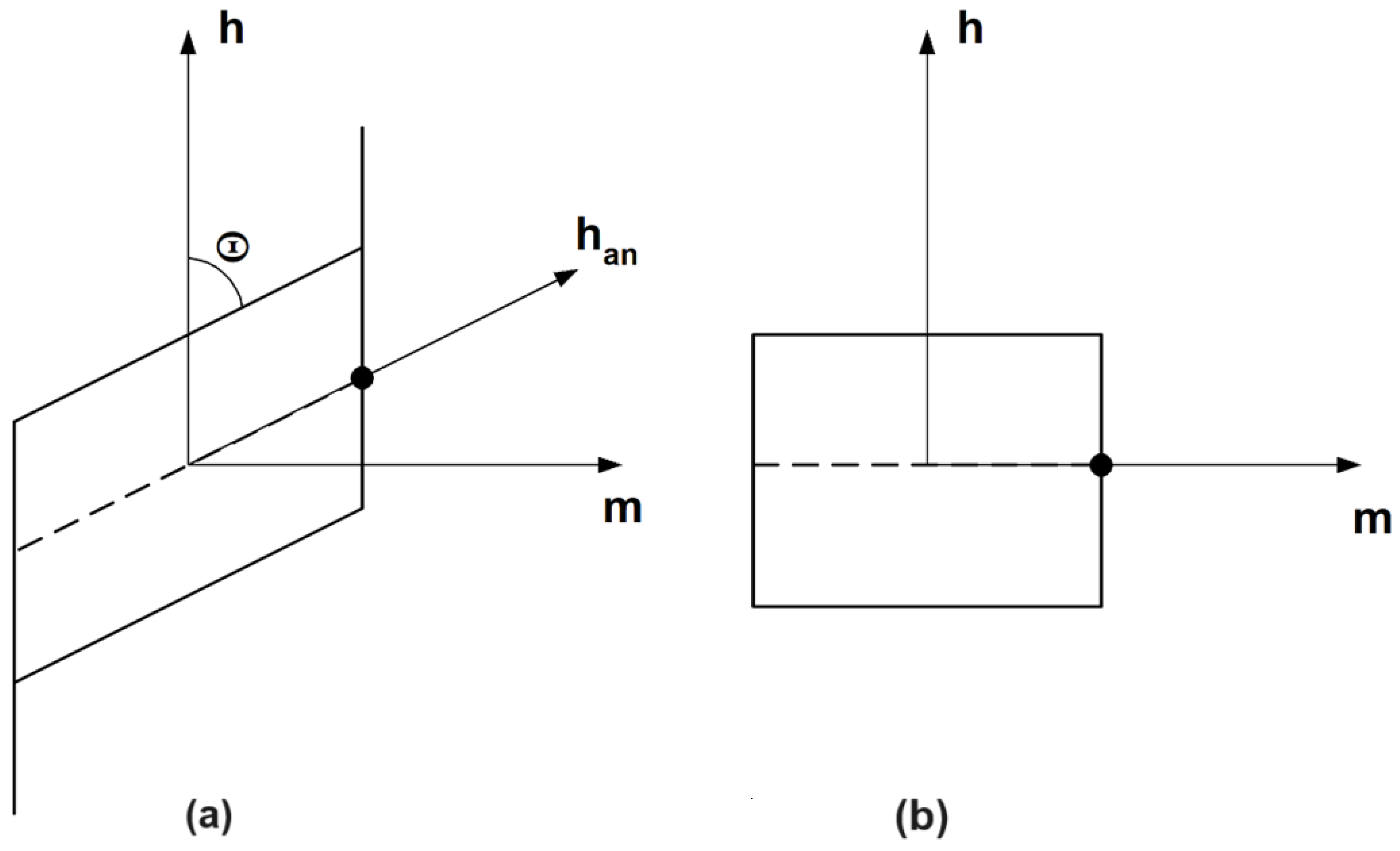
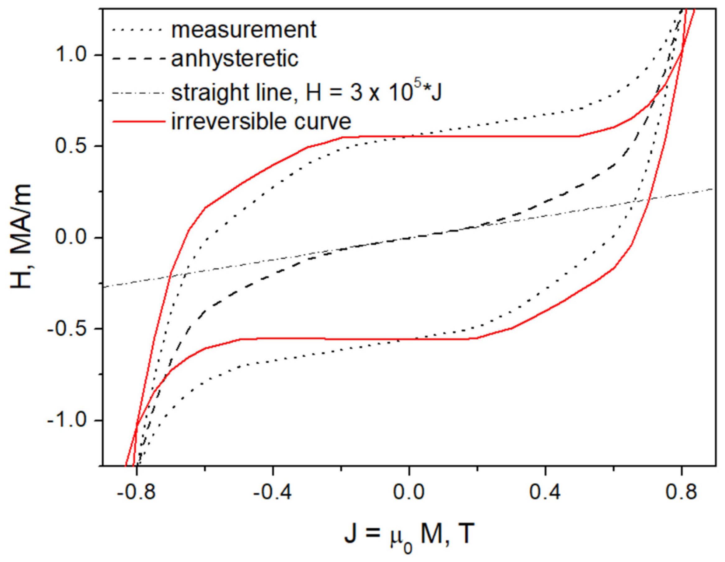
In the Harrison model, the role of the anhysteretic curve is merely to introduce a skewing of the coordinate system, which means a virtual contraction of the coordinate related to field strength. This can be appreciated in the example of a point marked with a black dot in Figure 6, which originally has non-zero field value but becomes the remanence point in the irreversible field vs. magnetization coordinate system.
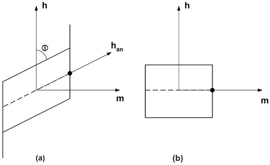
Figure 6.
The affine transformation based on angle ; (a)—measured hysteresis loop, (b) irreversible hysteresis loop. Solid lines—hysteresis loop, dashed line—anhysteretic curve (approximate shapes). The figure may be compared to Figure 5 in [10] or Figure 10 in [39].
A similar affine transformation was considered recently in [39]. If addition of irreversible and reversible field strength components holds, then the reverse processing of experimental hysteresis loops is also possible. Therefore, the irreversible hysteresis loops may also be recovered from the measured ones using an affine transformation where the angle marked as in Figure 6 is related to a measurable quantity, i.e., the reciprocal of dynamic susceptibility at coercivity (, and we are concerned with a transformation of the axis clockwise by the complementary angle so that it overlaps the axis.
The transformation matrix which may be used for computation of coordinates of points belonging to the irreversible loop marked as (b) may be written as:
and its inverse as:
The forward transformation may also be interpreted as an attempt to force the straight line with non-zero slope equal to the reciprocal of differential anhysteretic susceptibility to be aligned with the axis.
The afore-given transformation can be also used in the analysis of magnetic circuits with open air gaps, which introduce “skewing” of M–H dependencies.
3. Results
Exemplary modeling was carried out for a Pr8Dy1Fe60Co7Ni6B14Zr1Ti3 ribbon (a hard magnet, examined previously in [9]). The details on sample preparation are provided in [42]. Figure 7 depicts the decomposition of the measured hysteresis loop into the irreversible hysteresis loop related to the bistability phenomenon and the anhysteretic curve in accordance with the approach outlined in the previous section.
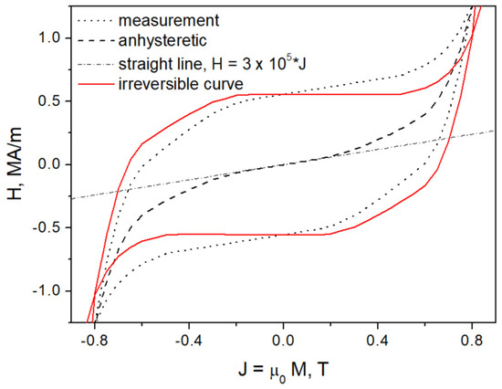
Figure 7.
The decomposition of measured hysteresis loop into irreversible and reversible components.
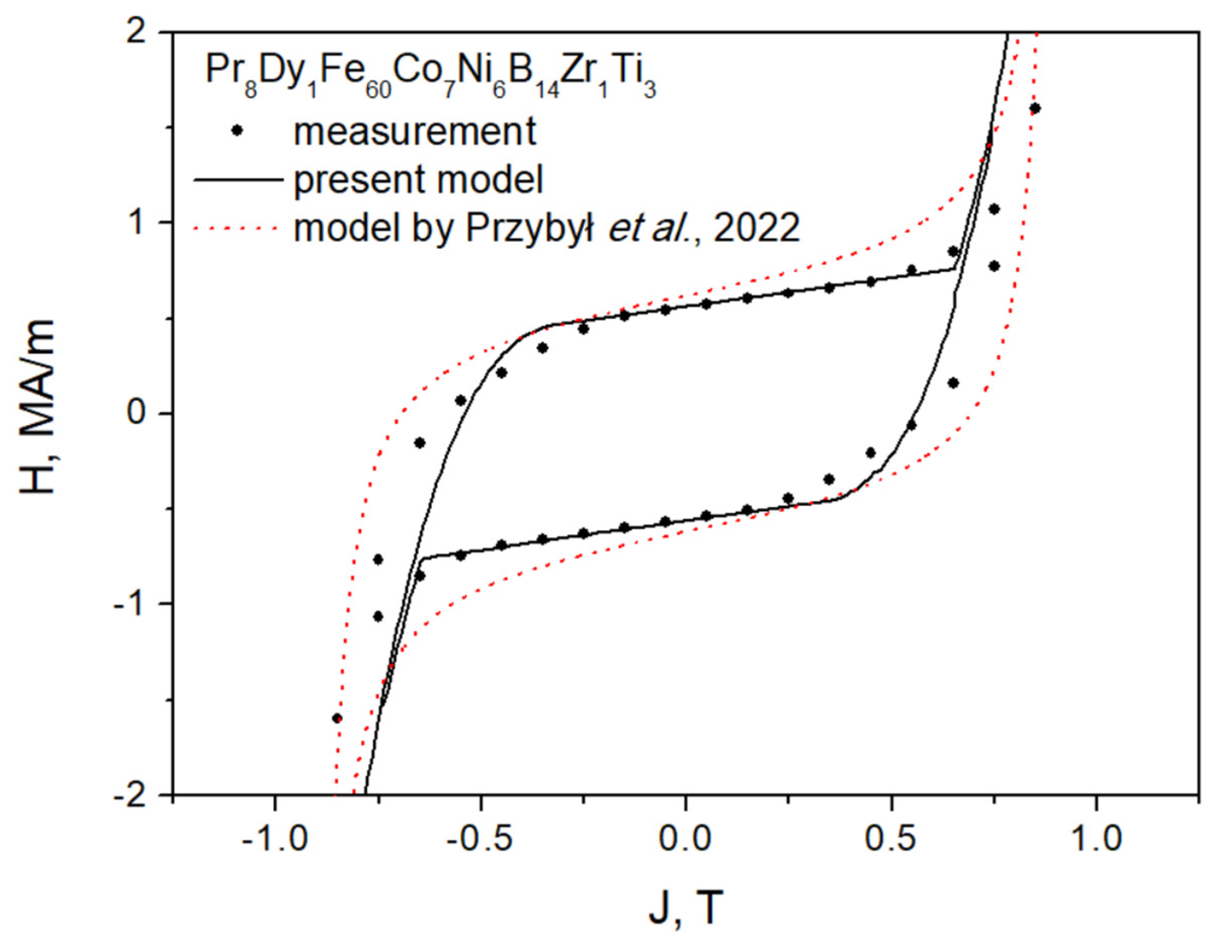
In modeling, we considered just two hysterons without weighting to make the structure really simple; the dependence generating bistability for the first hysteron was . The other unit was of type (5), where the value of the parameter was taken as . The results of modeling are presented in Figure 8. It can be stated that, despite its simplicity, the model is able to capture the shape of the measured hysteresis curves quite well, which may be inferred from a visual comparison with previous modeling results [9] (drawn with red dotted lines). It is noticeable that the shape of the measured hysteresis curve is better reproduced with the new approach. The J–H dependencies modeled with the original model from [9] generally overestimated the values which may be considered “figures of merit”, i.e., coercivity and remanence polarization, and the shapes of modeled hysteresis curves remained in qualitative agreement with the experiment. In terms of quantitative assessment, the discrepancy between coercive field strength modeled with the present model and its experimental counterpart is merely 1.05%; this value should be compared to 11.4% discrepancy for the model from [9] and the experimental value for this specific point. For remanence polarization, the respective discrepancy values are 11.4% (the present model) and 17.2% (model from [9]).
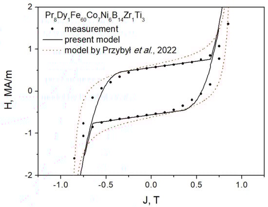
Figure 8.
The measured (dots) and the modeled (solid lines) hysteresis curves. Additionally, the modeling results for the same sample from Ref. [9] (Przybył et al., 2022) are shown as red dotted lines.
The present model works much better, particularly for lower values of magnetic flux density, and the value of coercive field strength is very well reproduced. The departures of modeled hysteresis curves from the experimental data points around the “knee” and in the region approaching saturation may be due to the arbitrary choice of hysterons with specified characteristics and considering just two of them. We believe that much better accuracy may be achieved if more units are taken into account. It is evident that use of many hysterons in the analysis results in better capability of reproducing experimental results (due to increased number of degrees of freedom of the description—this explains the successful story of the Preisach formalism); on the other hand, we wanted to keep the model structure as simple as possible in our preliminary tests.
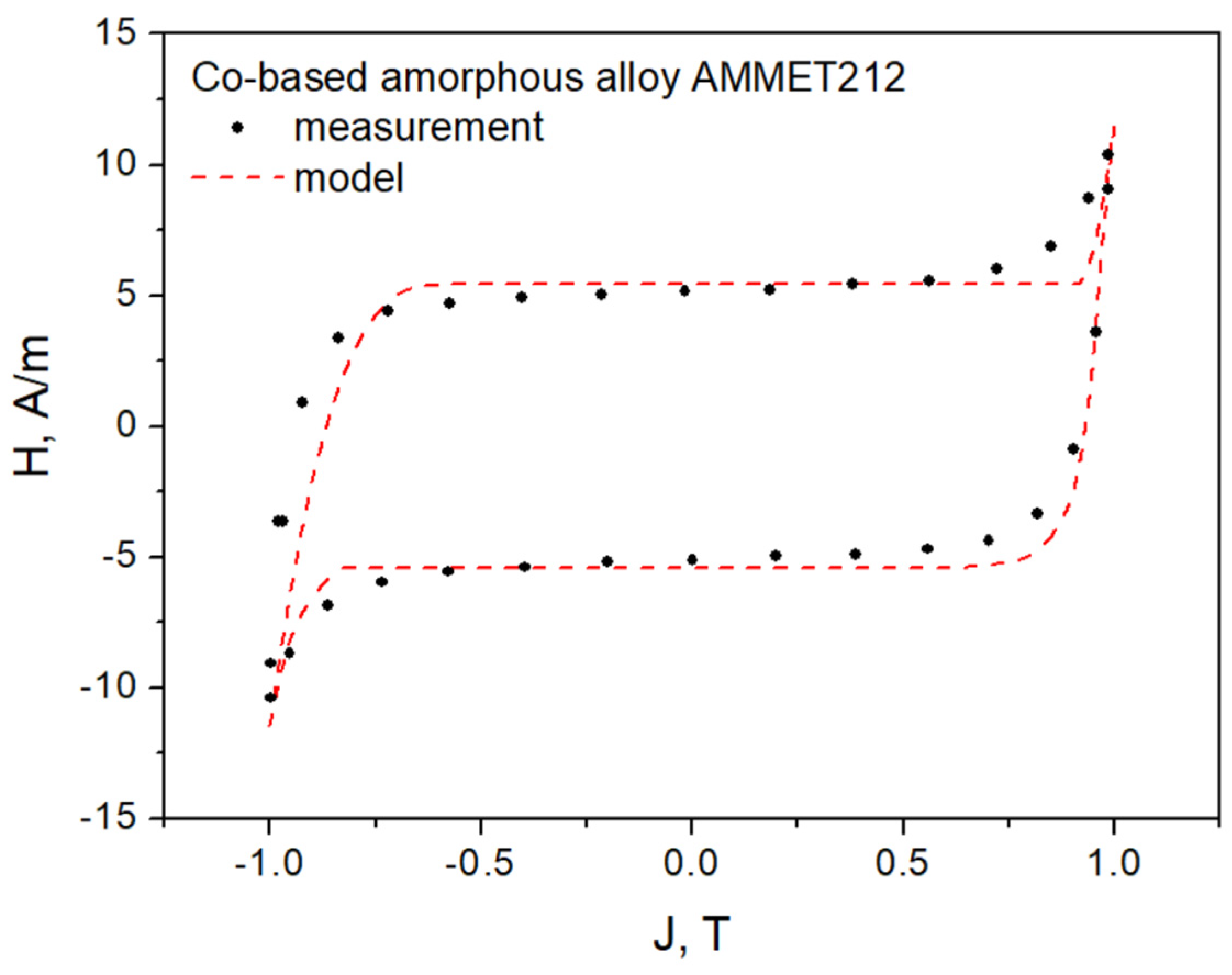
As a second attempt to apply the developed description in practice, we carried out modeling for a cylinder core wound of Co-based amorphous alloy AMMET212. As pointed out by Harrison, his approach should be valid both for soft and hard magnetic materials. The considered material is extremely soft since the measured value of coercive field strength is 5.1 A/m (this is a value five order of magnitude lower than for the praseodymium–dysprosium sample shown in Figure 8). Again, we considered a combination of just two hysterons. The J–H dependency of the first one was given with expression (7); for the other one, it was of similar type, yet with different values of coefficients, i.e.,
For the latter hysteron, , and the bifurcation magnetization , whereas the corresponding value of field strength (coercive field strength)
The value of magnetization when two branches of a hysteresis loop coincide is approximately
The results of modeling are depicted in Figure 9. During modeling, no weighting of hysteron outputs was assumed.
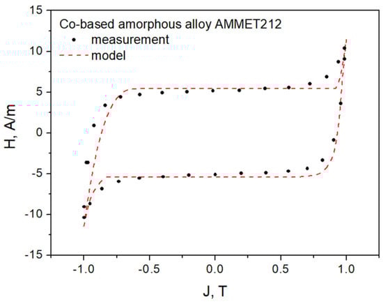
Figure 9.
The measured (dots) and the modeled (solid lines) hysteresis curves for a cobalt-based amorphous alloy.
4. Conclusions
Summing up to this point, in this contribution we have presented the following concepts:
- -
- The phenomenological parameter introduced by Harrison is abandoned since it implies averaging and oversimplifies the model, which affects its usefulness;
- -
- The response of elementary hysteretic units (“hysterons”) is considered in a similar way as in the stop model;
- -
- Some analytical relationships which might be used for the description are provided;
- -
- It is possible to consider distributions of parameters used in the description of hysterons which bear a striking similarity to the Preisach formalism; however, the presented approach works as an inverse model, and thus the necessity to post-process the computation results [43,44,45] is avoided;
- -
- The possibility to recover the irreversible hysteresis loop from the experimental curves is outlined;
- -
- The affine transformation between the natural (related to measurements) coordinate system and its counterpart, in which magnetization is related to the slope of the anhysteretic curve, and, subsequently, to the slopes of hysteresis curves at coercivity, are explained;
- -
- A verification of the methodology is carried out using previously published data concerning praseodymium–dysprosium ribbon (an example of a hard magnet) and for a cylinder core wound of cobalt-based amorphous alloys (an example of an extremely soft magnetic material).
Future work shall be focused on developing a reliable identification method for the proposed generalized stop model. Moreover, we plan to carry out an in-depth study on the constraints and dependencies between the values of polynomials which can serve as building blocks for hysterons. Subsequently, the study might shed some light on the descriptions of more complicated energy landscapes, which can include multi-stability as well. As we have pointed out in Section 2, the goal of this paper was to demonstrate that a better modeling accuracy and flexibility may be obtained for the modified Harrison model. On the other hand, we think that the presence of different hysterons might be interpreted in terms of the existence of phases present in real-life material. This issue shall be explored in subsequent studies.
Author Contributions
Conceptualization, K.C., P.G. and R.G.; methodology, K.C.; software, A.P.S.B. and B.S.R.; validation, A.P., A.P.S.B. and B.S.R.; formal analysis, K.C.; investigation, P.G. and A.P.; resources, A.P.; data curation, A.P.; writing—original draft preparation, K.C.; writing—review and editing, A.P.S.B. and B.S.R.; visualization, K.C., P.G. and R.G.; supervision, K.C.; project administration, K.C.; funding acquisition, K.C. All authors have read and agreed to the published version of the manuscript.
Funding
This research received no external funding.
Institutional Review Board Statement
Not applicable.
Informed Consent Statement
Not applicable.
Data Availability Statement
The data presented in this study are available on request from the corresponding author. The data are not publicly available because they are still being analysed for their usability in a potential new paper.
Conflicts of Interest
The authors declare no conflict of interest.
References
- Noori, M.; Altabey, W.A. Hysteresis in Engineering Systems (Editorial). Appl. Sci. 2022, 12, 9428. [Google Scholar] [CrossRef]
- De Santis, V.; Di Francesco, A.; D’Aloia, A.G. A Numerical Comparison between Preisach, J-A and D-D-D Hysteresis Models in Computational Electromagnetics. Appl. Sci. 2023, 13, 5181. [Google Scholar] [CrossRef]
- Bertotti, G. Hysteresis in Magnetism: For Physicists, Materials Scientists, and Engineers; Academic Press: San Diego, CA, USA, 1998. [Google Scholar]
- Mörée, G.; Leijon, M. Review of hysteresis models for magnetic materials. Energies 2023, 16, 3980. [Google Scholar] [CrossRef]
- Mörée, G.; Leijon, M. Review of Play and Preisach Models for Hysteresis in Magnetic Materials. Materials 2023, 16, 2422. [Google Scholar] [CrossRef]
- Gębara, P.; Gozdur, R.; Chwastek, K. The Harrison Model as a Tool to Study Phase Transitions in Magnetocaloric Materials. Acta Phys. Pol. A 2018, 134, 1217–1220. [Google Scholar] [CrossRef]
- Chwastek, K.; Gozdur, R. Towards a Unified Approach to Hysteresis and Micromagnetics Modeling: A Dynamic Extension to the Harrison Model. Phys. B Condens. Mat. 2019, 572, 242–246. [Google Scholar] [CrossRef]
- de Souza Dias, M.B.; Landgraf, F.J.G.; Chwastek, K. Modeling the Effect of Compressive Stress on Hysteresis Loop of Grain-Oriented Electrical Steel. Energies 2022, 15, 1128. [Google Scholar] [CrossRef]
- Przybył, A.; Gębara, P.; Gozdur, R.; Chwastek, K. Modeling of Magnetic Properties of Rare-Earth Hard Magnets. Energies 2022, 15, 7951. [Google Scholar] [CrossRef]
- Harrison, R.G. A Physical Model of Spin Ferromagnetism. IEEE Trans. Magn. 2003, 39, 950–960. [Google Scholar] [CrossRef]
- Weiss, P. L’hypothèse du champ moléculaire et la propriété ferromagnétique (The hypothesis of molecular field and ferromagnetic property). J. Phys. Theor. Appl. 1907, 6, 661–690. (In French) [Google Scholar] [CrossRef]
- Mohn, P. Magnetism in the Solid State. An Introduction; Springer: Berlin/Heidelberg, Germany, 2006. [Google Scholar]
- Cullity, B.D.; Graham, C.D. Introduction to Magnetic Materials, 2nd ed.; IEEE Press: Piscataway, NJ, USA; John Wiley & Sons: Hoboken, NJ, USA, 2009. [Google Scholar]
- Kliem, H.; Kuehn, M.; Martin, B. The Weiss Field Revisited. Ferroelectrics 2010, 400, 41–51. [Google Scholar] [CrossRef]
- Jiles, D.C.; Atherton, D.L. Theory of Ferromagnetic Hysteresis. J. Magn. Magn. Mater. 1986, 61, 48–60. [Google Scholar] [CrossRef]
- Vicsek, T. A Question of Scale. Nature 2001, 411, 421. [Google Scholar] [CrossRef] [PubMed]
- Kobayashi, T.; Onaga, T. Dynamics of Diffusion on Monoplex and Multiplex Networks: A Message-passing Approach. Econ. Theory 2023, 76, 251–287. [Google Scholar] [CrossRef]
- Zhao, Y.Q. Statistical Inference for Mean Field Queuing Models. Queueing Syst. 2022, 100, 569–571. [Google Scholar] [CrossRef]
- Yuan, Z. Self-supervised End-to-end Graph Local Clustering. World Wide Web 2023, 26, 1157–1179. [Google Scholar] [CrossRef]
- Furusawa, T. Mean Field Theory in Deep Metric Learning. arXiv 2023, arXiv:2306.15368. [Google Scholar] [CrossRef]
- Schneider, C.S.; Winchell, S.D. Hysteresis in Conducting Ferromagnets. Phys. B 2006, 372, 269–272. [Google Scholar] [CrossRef]
- Íñiguez, J.; Zubko, P.; Luk’yanchuk, I.; Cano, A. Ferroelectric Negative Capacitance. Nat. Rev. Mater. 2019, 4, 243–256. [Google Scholar] [CrossRef]
- Hoffmann, M.; Fengler, F.P.G.; Herzig, M.; Mittmann, T.; Max, B.; Schroeder, U.; Negrea, R.; Lucian, P.; Slesazeck, S.; Mikolajick, T. Unveiling the Double-well Energy Landscape in a Ferroelectric Layer. Nature 2019, 565, 464–467. [Google Scholar] [CrossRef]
- Helmiss, G.; Storm, L. Movement of an Individual Bloch Wall in Single-crystal Picture Frame of Silicon Iron at Very Low Velocities. IEEE Trans. Magn. 1974, 10, 36–38. [Google Scholar] [CrossRef]
- Bobbio, S.; Miano, G.; Serpico, C.; Visone, C. Models of Magnetic Hysteresis Based on Play and Stop Hysterons. IEEE Trans. Magn. 1997, 33, 4417–4426. [Google Scholar] [CrossRef]
- Matsuo, T.; Terada, Y.; Shimasaki, M. Stop Model With Input-Dependent Shape Function and Its Identification Methods. IEEE Trans. Magn. 2004, 40, 1776–1783. [Google Scholar] [CrossRef]
- Zhou, C.; Feng, C.; Aye, Y.N.; Ang, W.T. A Digitized Representation of the Modified Prandtl–Ishlinskii Hysteresis Model for Modeling and Compensating Piezoelectric Actuator Hysteresis. Micromachines 2021, 12, 942. [Google Scholar] [CrossRef] [PubMed]
- Landau, L.D. On the theory of phase transitions. Zh. Eksp. Teor. Fiz. 1937, 7, 19–32. Available online: https://web.archive.org/web/20151214124950/ (accessed on 10 September 2023). (In Russian). [CrossRef]
- Kádár, G. On the Preisach Function of Ferromagnetic Hysteresis. J. Appl. Phys. 1987, 61, 4013–4015. [Google Scholar] [CrossRef]
- Della Torre, E. Magnetic Hysteresis; Wiley: Hoboken, NJ, USA; IEEE Press: Piscataway, NJ, USA, 1998. [Google Scholar]
- Cao, Y.; Xu, K.; Jiang, W.; Droubay, T.; Ramuhalli, P.; Edwards, D.; Johnson, B.R.; McCloy, J. Hysteresis in single and polycrystalline iron thin films: Major and minor loops, first order reversal curves, and Preisach modeling. J. Magn. Magn. Mater. 2015, 395, 361–375. [Google Scholar] [CrossRef]
- Miller, J. CUPID: A MATLAB Toolbox for Computations with Univariate Probability Distributions. 16 December 2022. Available online: https://github.com/milleratotago/Cupid (accessed on 7 September 2023).
- Zirka, S.E.; Moroz, Y.I.; Harrison, R.G.; Chwastek, K. On physical aspects of the Jiles-Atherton hysteresis models. J. Appl. Phys. 2012, 112, 043916. [Google Scholar] [CrossRef]
- Koltermann, P.I.; Righi, L.A.; Bastos, J.P.A.; Carlson, R.; Sadowski, N.; Batistela, N.J. A modified Jiles method for hysteresis computation including minor loops. Phys. B Condens. Matter 2000, 275, 233–237. [Google Scholar] [CrossRef]
- Gozdur, R.; Gębara, P.; Chwastek, K. Modeling hysteresis curves of La(FeCoSi)13 compound near the transition point with the GRUCAD model. Open Phys. 2019, 16, 266–270. [Google Scholar] [CrossRef]
- Silveyra, J.M.; Conde Garrido, J.M. On the Modeling of the Anhysteretic Magnetization of Homogenous Soft Magnetic Materials. J. Magn. Magn. Mater. 2021, 540, 168430. [Google Scholar] [CrossRef]
- Silveyra, J.M.; Conde Garrido, J.M. On the Anhysteretic Magnetization of Soft Magnetic Materials. AIP Adv. 2022, 12, 035019. [Google Scholar] [CrossRef]
- Krah, J.H.; Bergqvist, A.J. Numerical optimization of a hysteresis model. Phys. B Condens. Matter 2004, 343, 35–38. [Google Scholar] [CrossRef]
- Chwastek, K.R.; Jabłoński, P.; Kusiak, D.; Szczegielniak, T.; Kotlan, V.; Karban, P. The Effective Field in the T(x) Hysteresis Model. Energies 2023, 16, 2237. [Google Scholar] [CrossRef]
- Kokornaczyk, E.; Gutowski, M.W. Anhysteretic functions for the Jiles-Atherton model. IEEE Trans. Magn. 2015, 51, 7300305. [Google Scholar] [CrossRef]
- Steentjes, S.; Petrun, M.; Glehn, G.; Dolinar, D.; Hameyer, K. Suitability of the double Langevin function for description of anhysteretic magnetization curves in NO and GO electrical steel grades. AIP Adv. 2017, 7, 056013. [Google Scholar] [CrossRef]
- Przybył, A.; Pawlik, K.; Pawlik, P.; Gębara, P.; Wysłocki, J.J. Phase composition and magnetic properties of (Pr, Dy)–Fe–Co–(Ni, Mn)–B–Zr–Ti alloys. J. Alloys Compd. 2012, 536 (Suppl. S1), S333–S336. [Google Scholar] [CrossRef]
- Takahashi, N.; Miyabara, S.-I.; Fujiwara, K. Problems in practical Finite Element analysis using Preisach hysteresis model. IEEE Trans. Magn. 1999, 35, 1243–1246. [Google Scholar] [CrossRef]
- Davino, D.; Giustiniani, A.; Visone, C. Fast Inverse Preisach Models in Algorithms for Static and Quasistatic Magnetic-Field Computations. IEEE Trans. Magn. 2008, 44, 862–865. [Google Scholar] [CrossRef]
- Bi, S.; Wolf, F.; Lerch, R.; Sutor, A. An Inverted Preisach Model with Analytical Weight Function and Its Numerical Discrete Formulation. IEEE Trans. Magn. 2014, 50, 7300904. [Google Scholar] [CrossRef]
Disclaimer/Publisher’s Note: The statements, opinions and data contained in all publications are solely those of the individual author(s) and contributor(s) and not of MDPI and/or the editor(s). MDPI and/or the editor(s) disclaim responsibility for any injury to people or property resulting from any ideas, methods, instructions or products referred to in the content. |
© 2023 by the authors. Licensee MDPI, Basel, Switzerland. This article is an open access article distributed under the terms and conditions of the Creative Commons Attribution (CC BY) license (https://creativecommons.org/licenses/by/4.0/).