Abstract
In this study, an analysis of coastal vulnerability and flood risk due to sea-level rise was conducted in the southern margin of the Ría of Arosa, Pontevedra (Spain), which is an area of urban impact and tourist activity. The vulnerability index was calculated using the following parametric maps: lithology, geomorphology, slope, elevation, distance, coastline change, significant wave height, sea level, and extreme tidal range. This vulnerability index was validated through the results obtained from the flood risk analysis, developed for different temporal and extreme scenarios (Xa—present, Xb—100 years, Xc—500 years, Xd—1000 years, Xe—storm, and Xf—tsunami). These analyses were performed using Geographic Information System and remote sensing techniques, spatial analysis, interpolation processes, and geostatistical analysis. The results of the analysis show the vulnerable areas and areas at high risk of coastal flooding, with the urbanized area exposed to a risk of 7.45 km2. Thus, this study contributes to designing appropriate management for the coastline of the southern margin of the Ría of Arosa in the event of a flood.
1. Introduction
Natural disasters have become more unpredictable and occur more frequently and forcefully due to climate change [1]. This climate change has led to an increase in the global average temperature [2], changes in the intensity and frequency of winds and waves [3], alterations in precipitation patterns [4], and variations in mean sea level [5]. Various studies by the Intergovernmental Panel on Climate Change (IPCC) indicate a sustained sea-level rise since the late 19th century, with a certain acceleration in the rate of rise during the second half of the 20th century. This trend has been recorded by various tide gauges since 1880, and confirmed through altimetric data collected by different satellites from 1993 to 2011. These studies have shown that the sea-level rise is approximately 3 mm per year [6,7,8].
Additionally, satellite data analyses have yielded diverse predictions for future sea-level rise in the 21st century, with rates ranging from 21–48 cm [6], 50–135 cm [5,6], 60–115 cm [9], 85–200 cm [10], 60–95 cm [11], 80–190 cm [12], 78–160 cm [11], to >100 cm [13]. Some projections suggest that in the 21st century and beyond, sea-level change will strongly influence regional patterns [14], with significant deviations in local and regional changes compared to the global average. Thus, during decadal periods, regional variation rates, due to climate variability, can differ by more than 100% from the global mean rate [14,15].
Coastal areas, in general, are threatened by hazards such as floods, erosion, and storms [1,2,3,4,5,6,7,8,9,10,11,12,13,14,15,16,17], and they will become more vulnerable in the future to the mentioned impacts of climate change. Furthermore, it is expected that the number of people living in coastal areas worldwide will increase from 1.8 to 5.2 billion by the 2080s [8,18,19]. As coastal systems become more complex from both social and environmental perspectives, the cost of damages caused by coastal hazards due to climate change impacts will also increase, making it essential to develop action strategies and raise awareness of these hazards [6,20,21,22].
Thus, the importance of awareness regarding coastal vulnerability is gaining attention among researchers and the public. Various vulnerability indices have been developed to study different impacts [23]. As a result, numerous studies on coastal vulnerability and flood risk have been conducted with the aim of evaluating these risks.
The coastline in the southern margin of the Ría of Arosa (the term “Ría” describes an estuary generated by an ancient coastal river valley that had been flooded by the sea during the Quaternary) is vulnerable to sea-level rise, particularly in beaches, marshes, and coastal wetlands. Human activity in these areas, especially tourism, poses additional challenges in terms of increasing vulnerability and exposure to hazards. Therefore, a study addressing short- and medium-term flood risk is necessary [24,25].
The objective of this work is to evaluate the degree of vulnerability and risk of coastal flooding by evaluating different characteristic factors for the study area. An innovative methodology is presented that allows the use of high-resolution and updated information, allowing the optimization of the data and the ease of calculation as new information is known. The vulnerability is calculated using the vulnerability index, which was developed by the United States Geological Survey (USGS), and which uses different intrinsic parameters of the coast studied using the Geographic Information System (GIS) ArcGis 10.8. For the analysis of flood risk, which is a function of the vulnerability of the studied area, deterministic methods are used, assigning a probability of sea-level rise based on a variety of foreseeable temporal scenarios (present (25 years), 100 years, 500 years, 1000 years, and extreme scenarios (storms and tsunamis)). This area was chosen due to its great tourist interest, which implies a large area of territory destined for urban uses due to its large influx of visitors, especially in the summer. The study will make it possible to reveal the areas of greatest vulnerability and/or risk of flooding so that the necessary preventive measures can be taken, both structural and non-structural. The latter measures are especially sensitive to this cartography.
2. Materials and Methods
2.1. Study Area
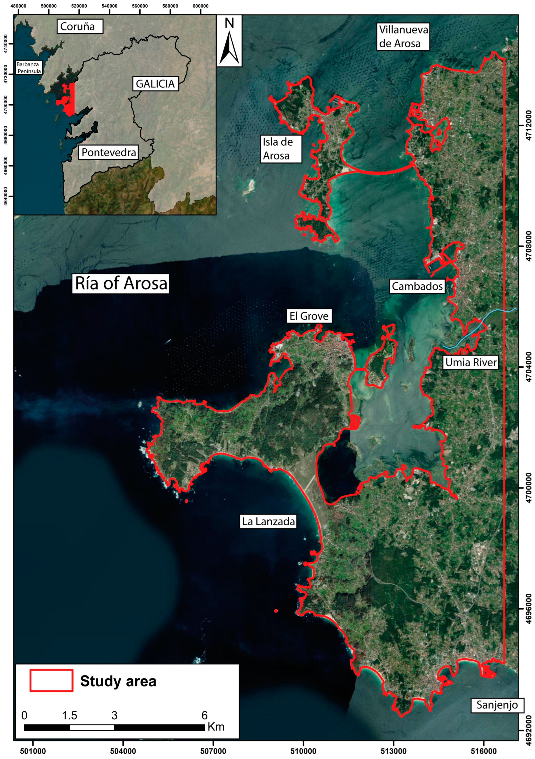
The study area is located in the northwest of the province of Pontevedra, on the southeastern coast of the Ría of Arosa (Figure 1). This ría is one of the largest and most important in the Rías Bajas, with its northern area belonging to the province of La Coruña and its southern area to the province of Pontevedra. In general, the study area covers approximately 9600 hectares and includes the Galician municipalities of Cambados, El Grove, and La Isla de Arosa, and parts of the municipalities of Sangenjo, Meaño, Ribadumia, and Villanueva de Arosa, where a total of 57,358 people reside. Climatologically, it is situated in a continental zone with Mediterranean influences that result in mild and humid average annual conditions [26]. The oceanic effect is the primary influencing factor for the mild temperatures and abundant precipitation. An average annual precipitation of approximately 1455 mm is recorded, with a mean summer temperature of 19.3 °C and 9 °C in winter [27].
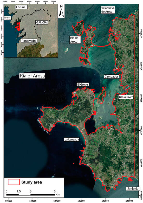
Figure 1.
Location map of the study area (in red) within the province of Pontevedra in Galicia.
The southeastern area of the Ría of Arosa is located in the northwest part of the Iberian Massif, specifically within the Galicia-Trás-os-Montes Zone. Geologically, it represents an internal zone of the Variscan orogeny and is characterized by being composed of various allochthonous domains overlying a bedrock of Paleozoic metasediments and granitic rocks. More precisely, the study area exhibits distinct lithological domains. The first domain is initially referred to as the Vigo–Pontevedra–Noya complex (“polymetamorphic graben” or “blastomylonitic trough”) and more recently referred to as the Malpica–Tui unit. It is a basal unit consisting of metasediments, including orthogneisses and metabasites. The deformation within the unit varies, with a dominance of highly deformed facies where mylonites can be observed. Structurally, it represents an elongated belt that covers almost the entire western part of Galicia. It is laterally bounded in the western part by a shear zone where it contacts the schistose or autochthonous domain, while in the eastern part, it is in contact with the para-autochthonous domain through a dextral-subvertical tear [28]. The autochthonous domain consists of metasediments and sandstones from the schist–graywacke complex, the mica schists of the “El Rosal-La Lanzada” region, and the two-mica alkaline feldspar granite of synkinematic nature from the “Villagarcía-Cuntis” region [28].
The western part of Galicia is dominated by a significant amount of granitic magmatism, representing the main typologies studied in the northwestern part of the Iberian Peninsula (Figure 2A). All these granites, in a simplified manner, can be classified according to their synkinematic and postkinematic nature. In the Barbanza Peninsula and on the Isla de Arosa, the postkinematic calc-alkaline granites belonging to the Caldas de Reyes pluton are best represented. This pluton exhibits multifacial characteristics ranging from biotite monzogranites to biotite granodiorites, with occasional occurrences of tonalite [29]. In the southeastern part of the study area, synkinematic calc-alkaline granites outcrop. In general, these granites appear as parallel and concordant bands with medium- to low-grade Variscan rocks. They exhibit deformation and local migmatization resulting from regional shear processes equivalent to the D3 evolutionary phase of the Variscan orogeny [30].
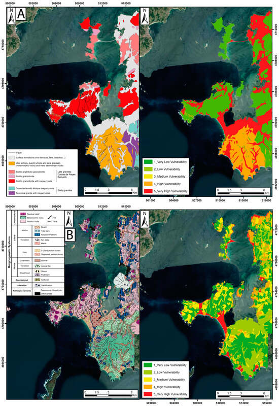
Figure 2.
(A) Lithological map (left) and its corresponding vulnerability map of the study area (right). Vulnerability values: metamorphic rocks, granodiorites, limestone and sandstone, metasediments, and Quaternary deposits. (B) Geomorphological map (left) and its respective vulnerability map (right). Vulnerability values: metamorphic and granitic rocks, alluvial and fluvial fans, slopes, fluvial reliefs, and foothills, fluvial and marine terraces, and endorheic areas, and all coastal sedimentary environments: beaches and dunes.
Geomorphologically, there are numerous well-defined geomorphological units grouped into different morphogenetic systems (Figure 2B). Several Quaternary units can be distinguished, which constitute the morphogenetic deposits of different depositional agents. These units are found overlying the Variscan basement. The structural conditions and transitional nature of the area allow for the development of various morphogenetic systems, with the lithological characteristics shaping the unique and specific relief of the Galician coastal zone, including the Ría of Arosa, and influencing the area’s morphogenesis.
The entire area is dominated by granitic lithologies that have been altered as a result of external geological processes, defining a granitic landform with mixed morphologies, divided based on their size. Large-scale morphologies, developed here in the two-mica granites, are represented by domes or bornhardts. These structures have a bell-shaped morphology, conditioned by orthogonal, curved, and radial fractures and joints within the body [31]. The reliefs dominated by these structures indicate a youthful attribute. In areas closer to the eastern margin of the ría, more evolved morphologies have undergone weathering (sandification) and more aggressive erosion, forming a more mature relief. The forms that appear here can range from tors to rock outcrops. The latter represent a more mature evolutionary stage compared to a dome. On the other hand, small-scale or minor morphologies are superimposed by all these large-scale ones, and are generated by subsurface processes. Examples of these structures can include gnamma pans, tafoni, or protruding walls.
The coastal or littoral system marks the transition between the aquatic and terrestrial environments. This transition does not occur abruptly but rather in a transitional manner. Therefore, three environments can be distinguished: marine, transitional, and aeolian (fully terrestrial). The marine environment encompasses two distinctly different processes: constructive and destructive. Constructive processes generate deposit or sedimentary forms, classified according to their origin: allochthonous (from fluvial systems), par-native (from aeolian processes and cliff erosion), and native (from biological activity). Under these conditions, the formation of beaches, tidal bars, tombolos, and coastal spits can develop. On the other hand, weathering and erosion will act in destructive processes, generating abrasion or planation surfaces. Structures originating in this environment can be marine terraces (former abrasion platforms subsequently uplifted by tectonic processes) and recent abrasion platforms. The origin of a relict abrasion platform can be marine or represent old polygenic surfaces exhumed by oceanic erosive processes [32].
Transitional environments represent areas where marshes and lagoons are affected by cyclic flooding. In these environments, low-energy constructive processes can be observed as a result of fine-grained sediment deposition. The aeolian environment consists of dune fields, and their mobility can vary depending on the vegetation they host.
2.2. Vulnerability Analysis of Coastal Flooding
Vulnerability is the extent to which geophysical, biological, and socioeconomic systems are susceptible and unable to cope with adverse impacts originating from environmental conditions or territorial elements [6].
To conduct a coastal vulnerability analysis of the study area, the Coastal Vulnerability Index (CVI) will be employed. The CVI, developed by the United States Geological Survey (USGS) [33], has been utilized in various subsequent coastal analyses along the Atlantic and Pacific coasts of the United States, as well as in studies of the Spanish coastline [15,34].
The USGS CVI method employs six parameters, whereas the index used in this study will incorporate ten parameters (Equation (1)), establishing the equation for the Ría de Arosa Vulnerability Index (IVRA):
where “Fl” represents the lithological factor; “Fg” denotes the geomorphological factor; “Fs” signifies the slope factor; “Fh” corresponds to the height factor; “Fd” stands for the distance factor; “Fb” represents the bathymetric factor; “Fc” indicates the coastal line change factor; “Fw” relates to the significant wave factor; “Fsl” pertains to the sea-level change factor; and “Ftr” represents the extreme tidal range factor.
IVRA = √(Fl × Fg × Fs × Fh × Fd × Fb × Fc × Fw × Fsl × Ftr)/10
By assigning five values to each parameter map, various vulnerability maps have been constructed for use in calculating the aforementioned index. A value of 1 will be assigned to the least vulnerable feature, while a value of 5 will be assigned to the most vulnerable feature. This weighting is depicted on a map with a cell size of 1 × 1 m, enabling a clear and detailed visual representation of the influence of each factor on the advancement of seawater towards the coastline.
2.2.1. Lithological Factor (Fl)
This factor indicates the resistance of lithological units to marine erosion. For the analysis of the lithological factor, geological materials are grouped into five classes based on their “hardness” in the face of potential water encroachment. The most recent unconsolidated materials (sand, gravel, etc.) have lower resistance to the effects of surface water, making them more vulnerable to sea encroachment than more consolidated lithologies such as metamorphic or igneous rocks. Therefore, the following vulnerability values are assigned: metamorphic rocks (value 1), granodiorites (value 2), limestones and sandstones (value 3), metasediments (value 4), and Quaternary deposits (value 5) (Figure 2A).
2.2.2. Geomorphological Factor (Fg)
As indicated by the previous factor, this one also provides information about the resistance of geomorphological units to marine erosion. The spatial distribution of geomorphological units and associated surface formations allows for the establishment of resistance levels based on their future location beneath the sea surface, revealing the degree of disintegration of each formation. Accordingly, the following vulnerability values are assigned: 1 to metamorphic and granitic rocks, 2 to alluvial fans and alluvial plains, 3 to pediments, fluvial reliefs, and piedmonts, 4 to river and marine terraces, as well as endorheic areas, and 5 to all coastal sedimentary environments, including beaches and dunes (Figure 2B).
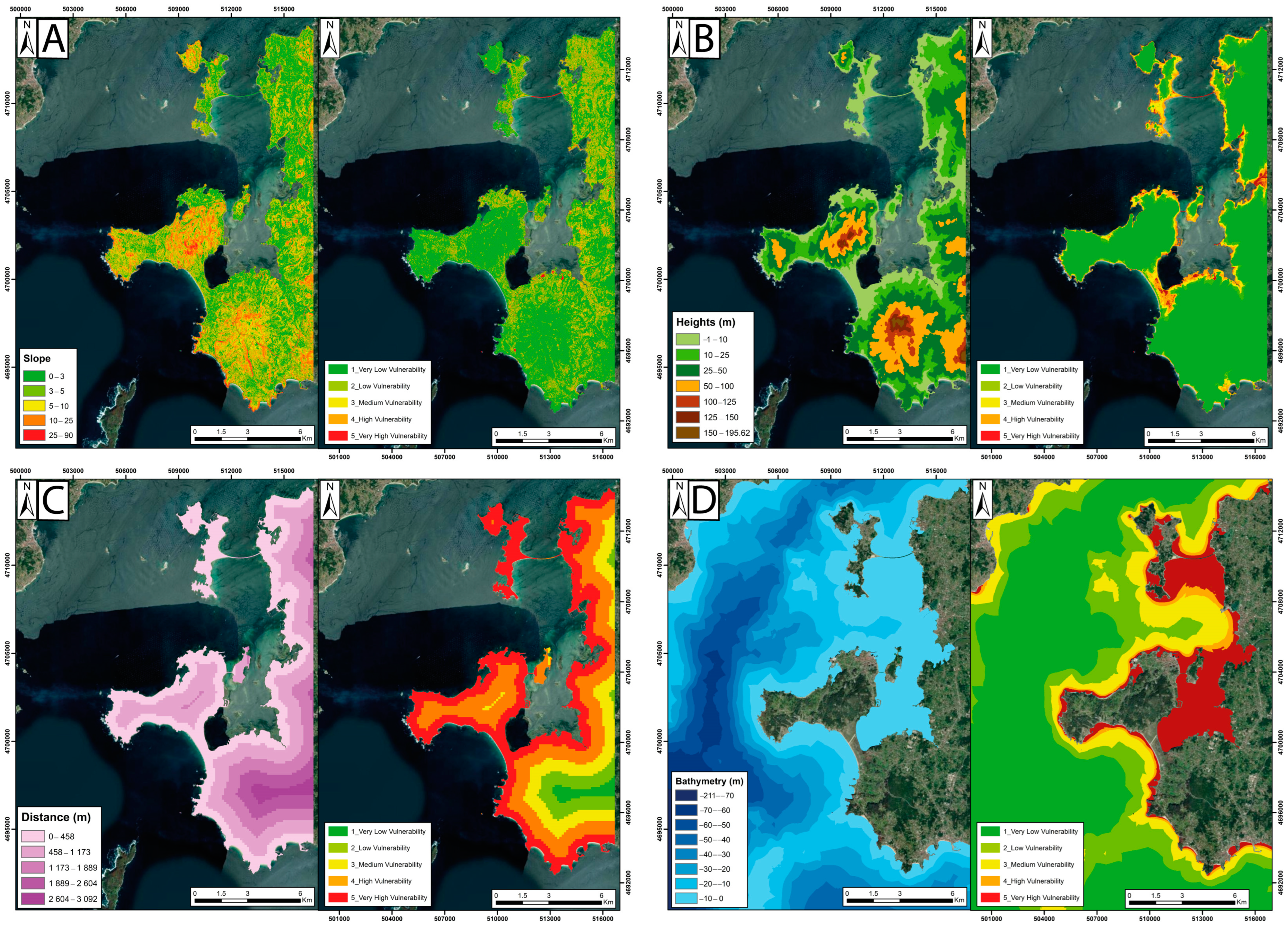
2.2.3. Slope Factor (Fs)
The terrain slope significantly influences inundation during a sea-level rise, also controlling the incline and speed of seawater retreat in the face of potential continental flooding [35]. To create the parameter map, a digital elevation model (DEM) is generated using 2015 Lidar data, where each pixel represents the elevation value, with a spatial resolution of 1 m. Vulnerability is weighted, considering that lower slopes are more vulnerable because seawater penetration is easier. Thus, 5 intervals are displayed indicating vulnerability for each pixel: 0–1% (value 5), 1–2% (value 4), 2–4% (value 3), 4–6% (value 2), and >6% (value 1) (Figure 3A).
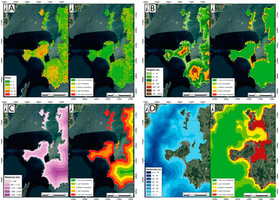
Figure 3.
(A) Slope map (left) and its corresponding vulnerability map (right). Vulnerability intervals: 0–1%, 1–2%, 2–4%, 4–6%, and >6%. (B) Altitude map of the study area (left) and its corresponding vulnerability map (right). Vulnerability intervals: 0–2 m, 2–4 m, 4–6 m, 6–10 m, and >10 m. (C) Distance map (left) and its corresponding vulnerability map (right). Vulnerability intervals: 0–458 m, 458–1173 m, 1173–1889 m, 1889–2604 m, and 2684–3092 m. (D) Bathymetric map of Ría of Arosa (left) and its corresponding vulnerability map (right). Vulnerability intervals: <1.5 m, 1.5–3 m, 3–10 m, 10–20 m, and >20 m.
2.2.4. Heigh Factor (Fh)
The height factor is one of the most important ones when assessing current risks related to sea-level rise. A 10-m elevation limit is considered unattainable based on current estimates of sea-level rise over the next 100 years [6]. Areas with elevations above 10 m will have low vulnerability levels, in contrast to areas near sea level (0 m) which will be more vulnerable. Thus, vulnerability gradually decreases as one moves inland. Vulnerability values are reclassified using the elevation values from the DEM, with the following height values for each pixel: 0–2 m (value 5), 2–4 m (value 4), 4–6 m (value 3), 6–10 m (value 2), and >10 m (value 1) (Figure 3B).
2.2.5. Distance Factor (Fd)
The distance factor estimates the ability of seawater to advance inland from the current coast of Ría de Arosa, as long as there is spatial continuity with the sea. This parameter calculates linear distances to the mainland from the 2017 coastline using the ArcGIS Map buffer tool. A raster layer was generated, and its data were reclassified based on standard deviation, with intervals of 0–458 m (value 5), 458–1173 m (value 4), 1173–1889 m (value 3), 1889–2604 m (value 2), and 2604–3092 m (value 1) (Figure 3C).
2.2.6. Bathymetric Factor (Fb)
The bathymetric factor determines the ease of greater or lesser marine encroachment on the coast, with greater progradation in deeper waters compared to shallow waters with less wave action, where the depth is less than half the wavelength causing wave drag. This factor provides information about the effect of waves on the beach and coastal ridges. The bathymetric map was created through data interpolation obtained from the EMODnet website. The reclassification of values was performed with the consideration that vulnerability will be high in shallow depths, as the action of breaking waves is more significant. The intervals are: <1.5 m (value 5), 1.5–3 m (value 4), 3–10 m (value 3), 10–20 m (value 2), and >20 m (value 1) (Figure 3D). Ría of Arosa is not a very deep area, as it does not exceed 70 m in depth.
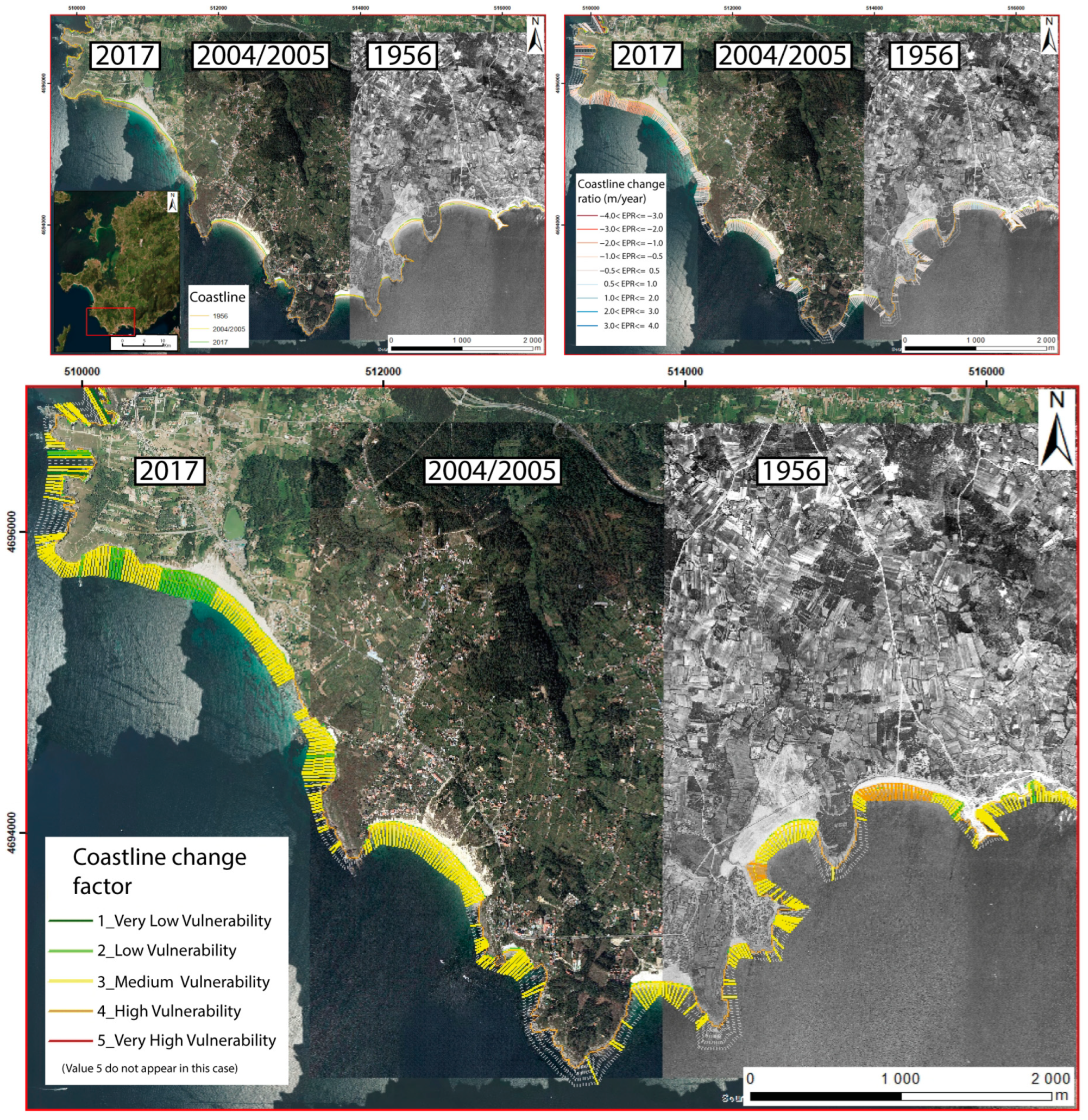
2.2.7. Coastal Factor/West Coastline Change Rate (Fc)
Coastal management for a section of coastline (e.g., hard coastal defenses, sediment input to the beach, or controlled realignment) is a key aspect in determining the long-term response of the coast to the impacts of climate change, including sea-level rise. Coastal erosion and coastal flooding are related through high water levels and energetic wave conditions during storms. Coastal geomorphology plays a crucial role here, as different types of morphology exhibit varying vulnerabilities, in addition to providing the pathway for coastal inundation [36].
The analysis of coastal evolution and morphological variations was carried out using GIS overlays, analyzing changes in the coastline over a 61-year period (1956–2017). This analysis is based on the overlay of aerial photographs from 1956 (coverage by American Flight—US Air Force) with a 1 m resolution and more recent orthophotographs from 2004–2005 and 2017, which were obtained from the National Geographic Institute’s National Aerial Orthophotography Plan (Figure 4). The positions of the coastlines were digitized and analyzed using the USGS-DSAS extension for ArcGIS v10.8, in terms of retreat or accretion rates (meters per year) during the mentioned periods (Figure 4). This tool allows for the analysis and quantification of changes in the coastline based on geospatial data and, in this case, is primarily used to study erosion and sediment accumulation in coastal areas [37].

Figure 4.
Analysis of coastal change. Vulnerability intervals: <−2.0, −2.0 to −1.0, −1.0 to 1.0, 1.0–2.0, and >2.0.
High growth values (coastline moving seaward) indicate high vulnerability, while negative rates (coastline retreating inland) indicate low vulnerability, with the following intervals in meters per year: <−2 (value 1), −2 to −1 (value 2), −1 to 1 (value 3), 1–2 (value 4), and >2 (value 5) (Figure 4). In general, there are moderate values (between −1 and 1 m per year) for coastline retreat along the entire Ría of Arosa coast.
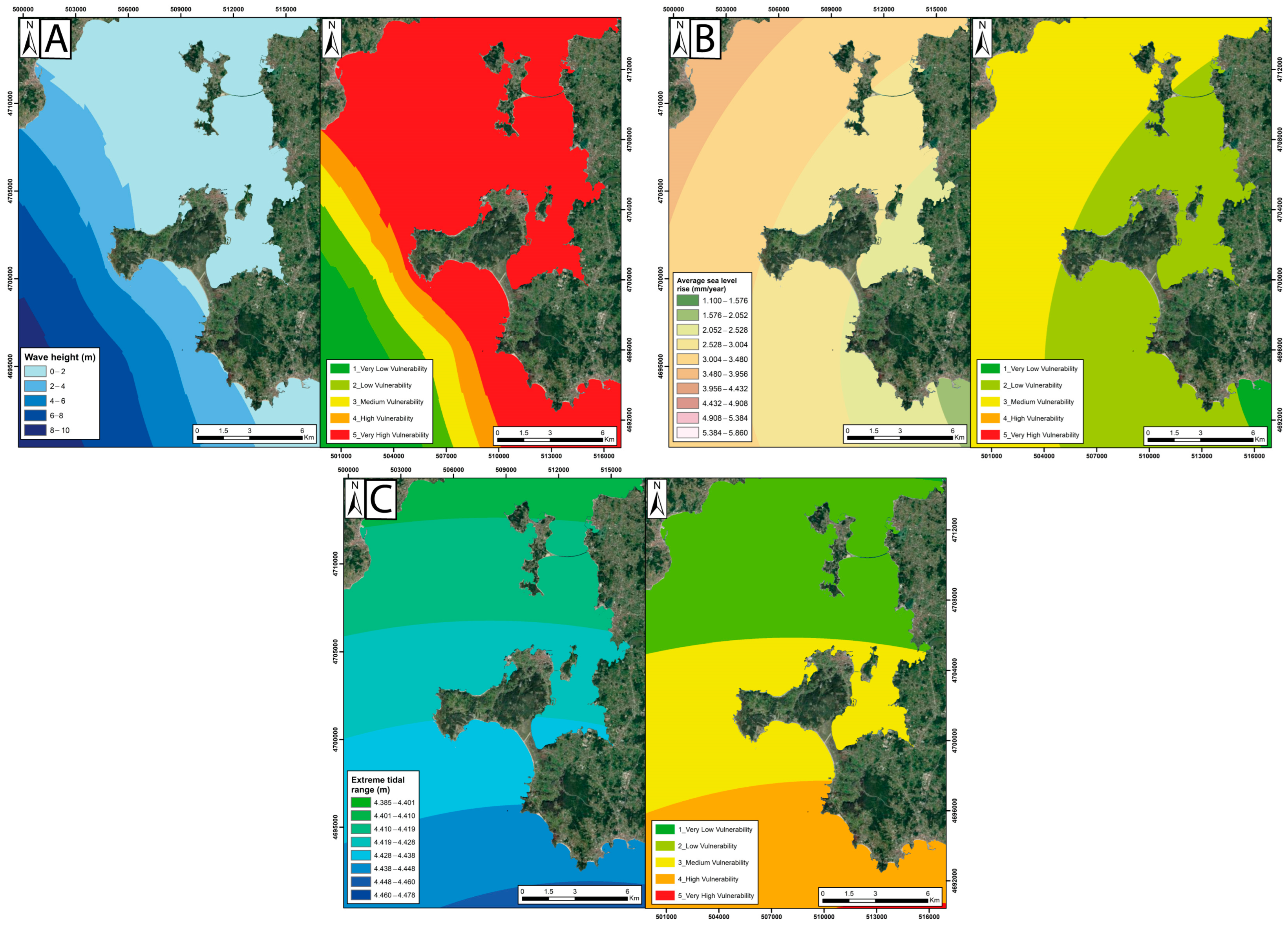
2.2.8. Wave Factor: Average Rate of Significant Waves (Fw)
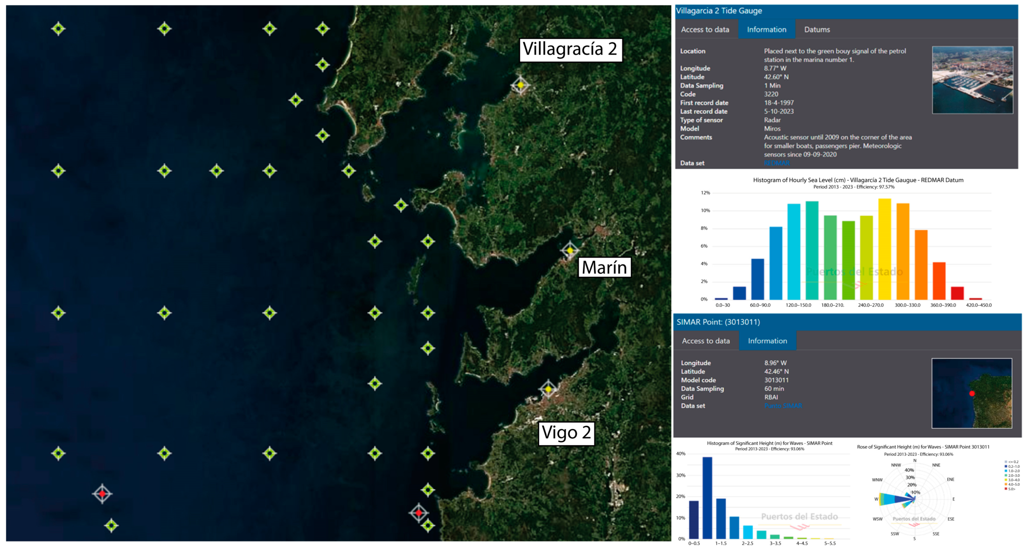
The wave factor indicates the maximum wave values that affect the coastline of Ría of Arosa, recorded at buoys located around the study area. These historical values have been obtained from the SIMAR dataset, retrieved from the Ports of State website (puertos.es) (Figure 5). The SIMAR dataset consists of time series of wind and wave parameters derived from numerical modeling, making them synthetic data and not directly measured from nature.
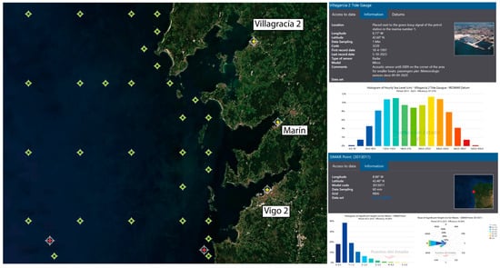
Figure 5.
Distribution of buoys (green marks), SIMAR points (red marks), and tide gauges (yellow marks) on the Ports of State website, along with an example of information view.
The SIMAR series arises from the amalgamation of two extensive datasets of simulated wave data historically maintained by Ports of State, namely, SIMAR-44 and WANA. Its primary goal is to provide more extensive and up-to-date temporal series. Consequently, the SIMAR dataset offers information dating back to the year 1958 and extending up to the present year, 2023. Through these data, valuable information about wave direction (Figure 5), peak and mean wave periods, and significant wave heights can be obtained. Notably, information on the latter is used to calculate the vulnerability factor for significant wave conditions. From among the significant wave height values, the highest data points for each SIMAR location are selected. This selection process aligns with the aim of this study, which is to statistically evaluate the most likely flooding risk, even in less frequent scenarios.
Once all significant wave heights from each SIMAR point were collected, the coordinates and data of the SIMAR points were entered into a Geographic Information System (GIS), and interpolation was performed. This allowed us to obtain a map of significant wave activity in the study area (Figure 6A). Considering that vulnerability is directly proportional to wave height, it can be assumed that the higher the wave, the greater the vulnerability in that area, and vice versa. Based on this assumption, the following vulnerability intervals have been established: 3.5–4 m (value 1), 4–5 m (value 2), 5–6 m (value 3), 6–7 m (value 4), and >7 m (value 5).
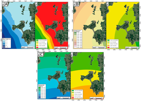
Figure 6.
(A) Map of significant wave heights in the study area (left) and its corresponding vulnerability map (right). Vulnerability intervals: 3.5–4 m, 4–5 m, 5–6 m, 6–7 m, and >7 m. (B) Map of sea-level change around the study area (left) and its corresponding vulnerability map (right). Vulnerability intervals in mm/year: 1.100–2.050, 2.051–3.000, 3.001–3.850, 3.851–4.910, and 4.911–5.860. (C) Map of extreme tidal range around the study area (left) and its corresponding vulnerability map (right). Vulnerability intervals in meters: 4.385–4.400, 4.401–4.420, 4.421–4.430, 4.431–4.450, and 4.451–4.478.
2.2.9. Sea-Level Factor (Fsl)
Through this factor, the relative sea-level change is analyzed using historical data recorded by tide gauges located near the study area. The data were sourced from the REDMAR dataset, which, as in the previous case, is available through Ports of State (Figure 5). The primary purpose of this dataset is to continuously measure, record, analyze, and store sea-level data in ports, with real-time data access being one of its key features. In this instance, data were obtained from the tide gauges in Villagarcía 2, Marin, and Vigo 2, resulting in different time series for each of them. Data for Villagarcía 2 and Vigo 2 cover the period from 1992 to 2021, while data for Marin spans the period from 2010 to 2021. Additionally, data from the Cascáis tide gauge, located in Portugal, were acquired through the PSMSL (Permanent Service for Mean Sea Level) website (psmsl.org), where international tide gauge data are archived. Historical data for this particular tide gauge extend from 1882 to 1993.
From the obtained data, the change in mean sea level was calculated for each tide gauge in millimeters, and these values were entered into and represented in a Geographic Information System (GIS). Interpolation was employed to generate a map depicting the average sea-level rise in the vicinity of the study area (Figure 6B). By reclassifying the acquired intervals, the following values were assigned: 1.1–2.05 (value 1), 2.05–3 (value 2), 3–3.96 (value 3), 3.85–4.91 (value 4), and 4.91–5.86 (value 5).
2.2.10. Extreme Tidal Range Factor (Ftr)
This factor analyzes the difference in height between high and low tides, with the tidal range varying from a few centimeters to several meters, depending on the geographical location of the tide gauge. As in the previous case, the data were obtained through the REDMAR dataset provided by Ports of State, including data for Villagarcía 2, Marin, and Vigo 2, as well as through the PSMSL website for the Cascáis tide gauge. Once the data was collected, it was input into a Geographic Information System (GIS), and interpolation was performed to generate the map of extreme tidal ranges in the study area. Despite the study area being located in a mesotidal regime (2–4 m), extreme tidal ranges exceeding 4 m were recorded. The vulnerability ranges assigned to the obtained values are as follows: 4.38–4.40 (value 1), 4.40–4.42 (value 2), 4.42–4.43 (value 3), 4.43–4.45 (value 4), and 4.45–4.47 (value 5) (Figure 6C).
2.3. Coastal Flooding Analysis
To support the results obtained through the vulnerability index, a coastal flood analysis of the study area was conducted using the Flood Hazard Index (FHI). Despite the last tsunami in Galicia being associated with the Lisbon earthquake of 1755, and the fact that the earthquake was more perceptible than the subsequent tsunami, Galicia is considered an exposed area to this natural hazard due to several proximal and distant focal mechanisms in the North Atlantic that could trigger a tsunami. These mechanisms include volcanic activity in the Azores and Madeira islands, seismic activity in the Mid-Atlantic Ridge, the Caribbean Plate, and the Azores-Gibraltar oceanic convergence zone, as well as large sediment masses mobilized along the North American coast. In the case of the Lisbon tsunami, maximum elevations of up to 3.3 m were recorded [38]. However, for this study involving extreme values, the maximum elevation reached by this tsunami on the coast was set to 8 m [39].
The coastal flood analysis is based on the parameters of significant wave height (Fw), sea-level change (Fsl), and extreme tidal range (Ftr), which are used to estimate flood hazard in different scenarios. The values for significant wave height and extreme tidal range are considered constant, while the sea-level change parameter values vary, capturing both minimum and maximum rates of rise (mm/year) from the interpolation conducted using Ports of State data.
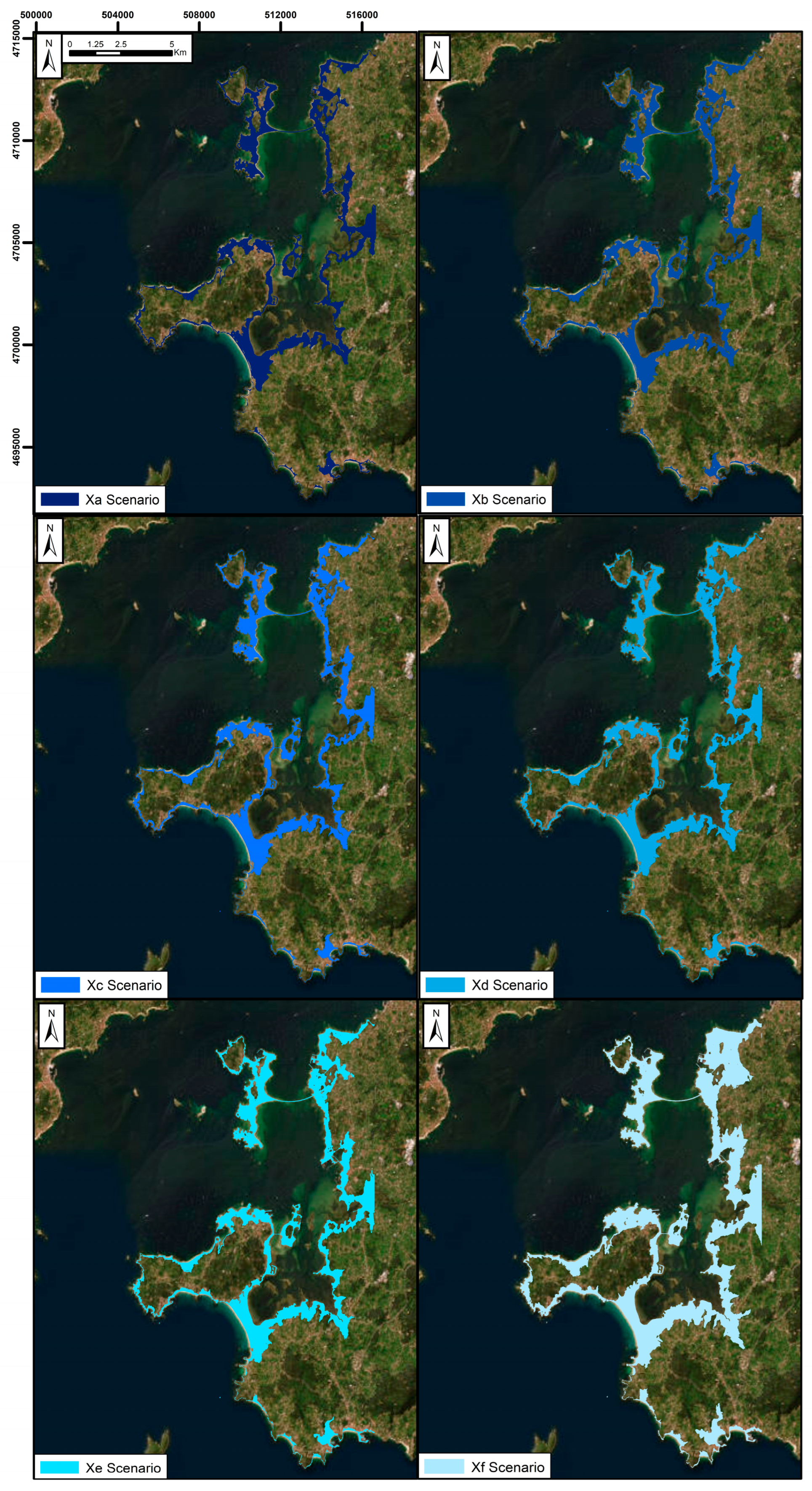
As a result, the scenarios used for flood risk analysis include present conditions, defined as a 25-year interval (Xa); 100 years (Xb); 500 years (Xc); 1000 years (Xd); and extreme storm (Xe) and tsunami (Xf) scenarios. These data and values are presented in Table 1, where summing the obtained values provides the maximum and minimum absolute extent of sea-level rise for each scenario.

Table 1.
Analyzed scenarios and their corresponding parameter values (in meters).
3. Results
3.1. Coastal Vulnerability in the Ría of Arosa
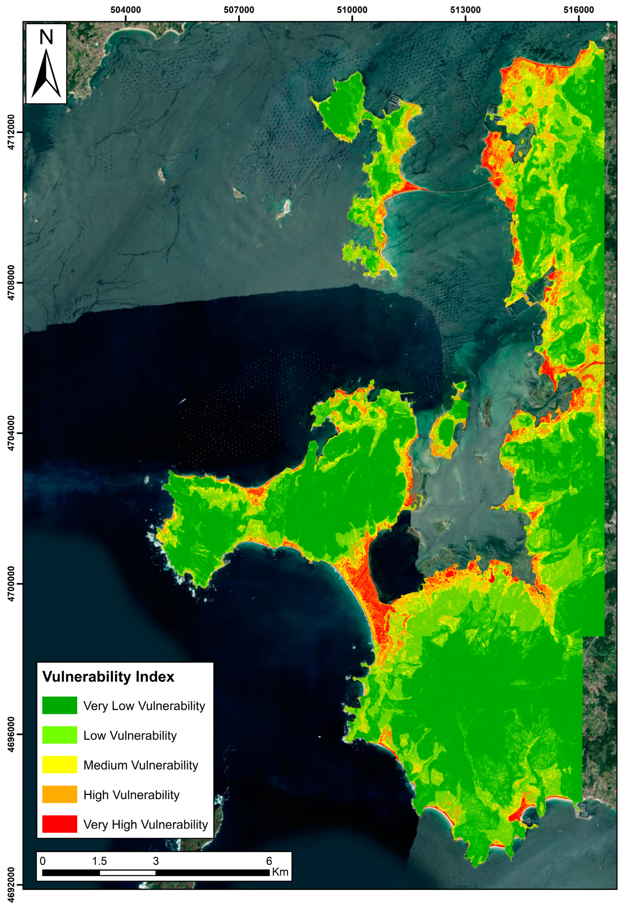
After obtaining all the parameters, the coastal vulnerability of the Ría of Arosa was calculated by modifying the vulnerability index developed by the USGS. To calculate the vulnerability index using the ArcGIS program, map algebra (raster calculator) was used to combine different parameters and generate the vulnerability map along the coast of the estuary (Figure 7). Therefore, a higher index indicates greater vulnerability to rising water levels.
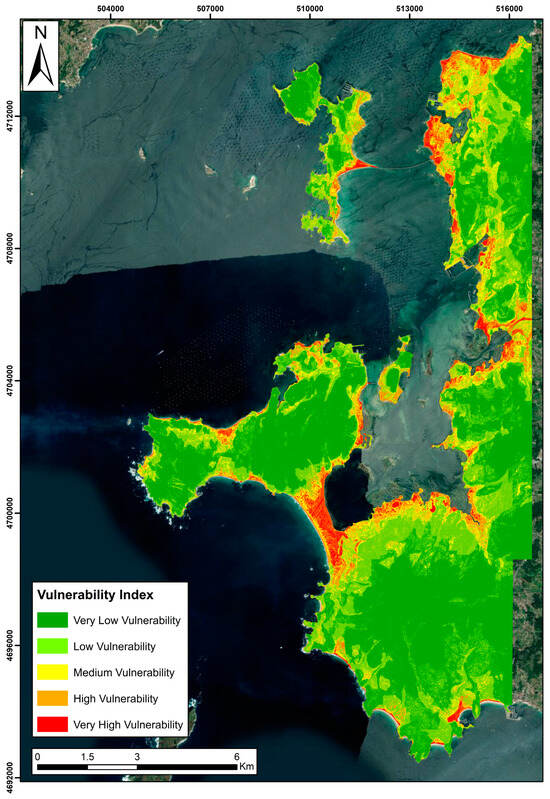
Figure 7.
Vulnerability index map of the Ría of Arosa. The higher the index obtained, the greater the vulnerability to rising water.
In general, a higher vulnerability can be observed near the coast, with vulnerability decreasing as one moves away from the coastline. Along the coastline, the highest vulnerability is often found in areas dominated by beaches and wetlands, while lower vulnerability is typically observed in cliff areas. When it comes to the most vulnerable localities, Sangenjo is considered the municipality with the highest vulnerability to sea-level rise, while El Grove or the Isla de Arosa exhibit the lowest vulnerability. Vulnerability can also be observed around the mouth of the Umia River and the tombolo of El Grove, where much of the area exhibits very high vulnerability.
In Villanueva de Arosa (Figure 7), the highest vulnerability is mainly concentrated along the coast, but it is worth noting that most of its pixels show a medium vulnerability. The most vulnerable areas in this locality are where there is no coastal protection, allowing water infiltration through the beaches in this area. However, urbanized areas protected by barriers or walls, such as the area near the port and the main urban core of the locality, show lower vulnerability values. In Cambados (Figure 7), high vulnerability values stand out in the floodplain of the Umia River, decreasing to medium and low values as one moves away from the flood-prone area. On the other hand, in the municipality of El Grove, predominantly low vulnerability values are found, increasing towards the coast but without significantly high vulnerability. However, it is observed that in the tombolo of El Grove (Figure 7), very high vulnerability prevails, making it the most vulnerable area in the entire study area. Finally, in the locality of Sangenjo (Figure 7), low vulnerability values predominate, with some high values in beach areas. Nevertheless, between Sangenjo and the locality of Portonovo, there is an area with very high vulnerability following the course of two streams that converge at the beach.
3.2. Coastal Flood Analysis of Ría of Arosa
Once the table of scenarios was complete, the maximum values obtained were used to generate flood risk maps for the coast of the Ría of Arosa. The sea-level rise scenarios were overlaid onto the orthophoto from the present year (2020), allowing for the visualization of various degrees of flood risk along the coast and areas with the highest water inundation potential in different scenarios (Figure 8).
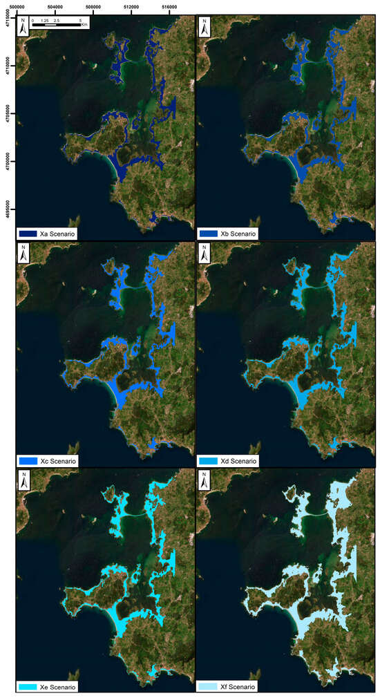
Figure 8.
Flood risk results for different scenarios.
It can be observed that, from scenario Xb to scenario Xe, there is no significant change in the extent reached by the sea level. This is because the difference in extent between these scenarios generally does not exceed one meter, with the minimum difference being 40 cm (from scenario Xd to scenario Xe) and the maximum difference being 80 cm (from scenario Xc to scenario Xd). In other words, the change is not very noticeable on the maps. However, the map of the extreme tsunami scenario (Xf) shows a significant change in extent, with a difference of 6 m when compared to the extreme storm scenario (Xe) and almost 8 m of difference when compared to the present situation (Xa).
In Villanueva de Arosa, there is not much variation in the extent of inundation between scenarios Xb and Xe, with most of the urbanized area near the sea being covered in scenario Xb (urban center, industrial areas, the port, etc.). With each subsequent scenario, the extent of water inundation expands over these urbanized areas. However, it is in scenario Xf where the most significant difference in extent can be observed, reaching urbanized areas further away from the coastline.
In Cambados, water inundation not only occurs from the sea but also from the Umia River, as this town is located near the mouth of the river. Most of the urbanized area near the coast is covered, with minimal variations in the first five scenarios, including urbanized areas (parts of the town center) further inland within the floodplain of the Umia River. Scenario Xf (tsunami) reaches urbanized areas further inland, both from the sea and the floodplain of the river. However, it does not extend to cover all urbanized areas in the town, leaving a significant portion unaffected.
In El Grove, scenarios Xb to Xe cover most of the urbanized areas along the coast. It can be observed that water infiltration is greater when it enters through a beach area than when it enters through a cliff area. In scenario Xf, the water covers more urbanized space but still does not reach some of the urbanized areas further inland from the coastline.
Lastly, in Sangenjo, it is worth noting that the most significant water infiltration occurs along two streams in the area, covering the urbanized areas near them. In the rest of the locality, the scenarios cover the ports but do not substantially inundate the other urban areas, with minimal variations in the extent of inundation in different scenarios. In the final scenario (Xf), the water covers more ground but still does not inundate the terrain more significantly than in the other scenarios.
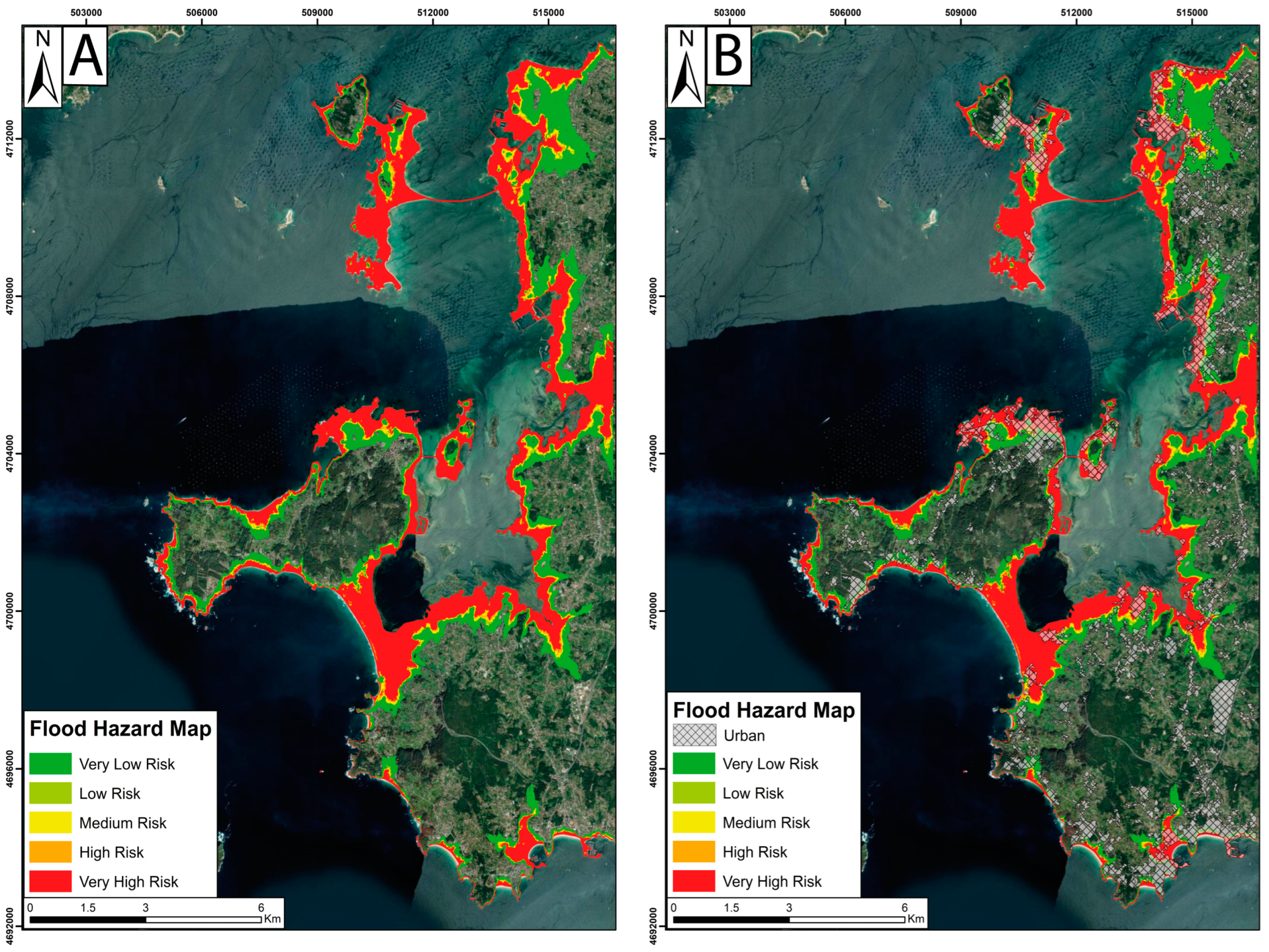
By weighting the different extents of water inundation based on their flood risk, the flood risk map of the SE sector of Ría of Arosa can be generated (Figure 9). As a result, the mainland area occupied by all scenarios will be the area with the highest flood risk (5), which is the zone closest to the sea. Conversely, the area covered by the fewest scenarios will represent the least vulnerable area (1), which, in this case, is represented by the extreme tsunami scenario (Xe) and is the zone furthest from the sea.

Figure 9.
(A) Flood risk map of SE sector of Ría of Arosa. (B) Flood risk map of the SE sector of the Ría de Arosa in which the urban areas have been added.
The flood risk map (Figure 9A) indeed exhibits similarities with the map obtained through the vulnerability index. As with the vulnerability index, the flood risk map shows higher risk in areas closer to the coast, while areas further inland have a lower risk of inundation. Overall, it can be observed that the tombolo of El Grove (where the Umia–O Grove intertidal complex is located), the Isla de Arosa, and the surroundings of the Umia River have a larger inundation area. Additionally, upon closer examination of the map, it is noteworthy that El Grove is at risk of the tombolo becoming submerged, effectively separating this municipality from the mainland and turning it into an island. Similarly, the Isla de Arosa is at risk of potentially becoming three separate islands in the future.
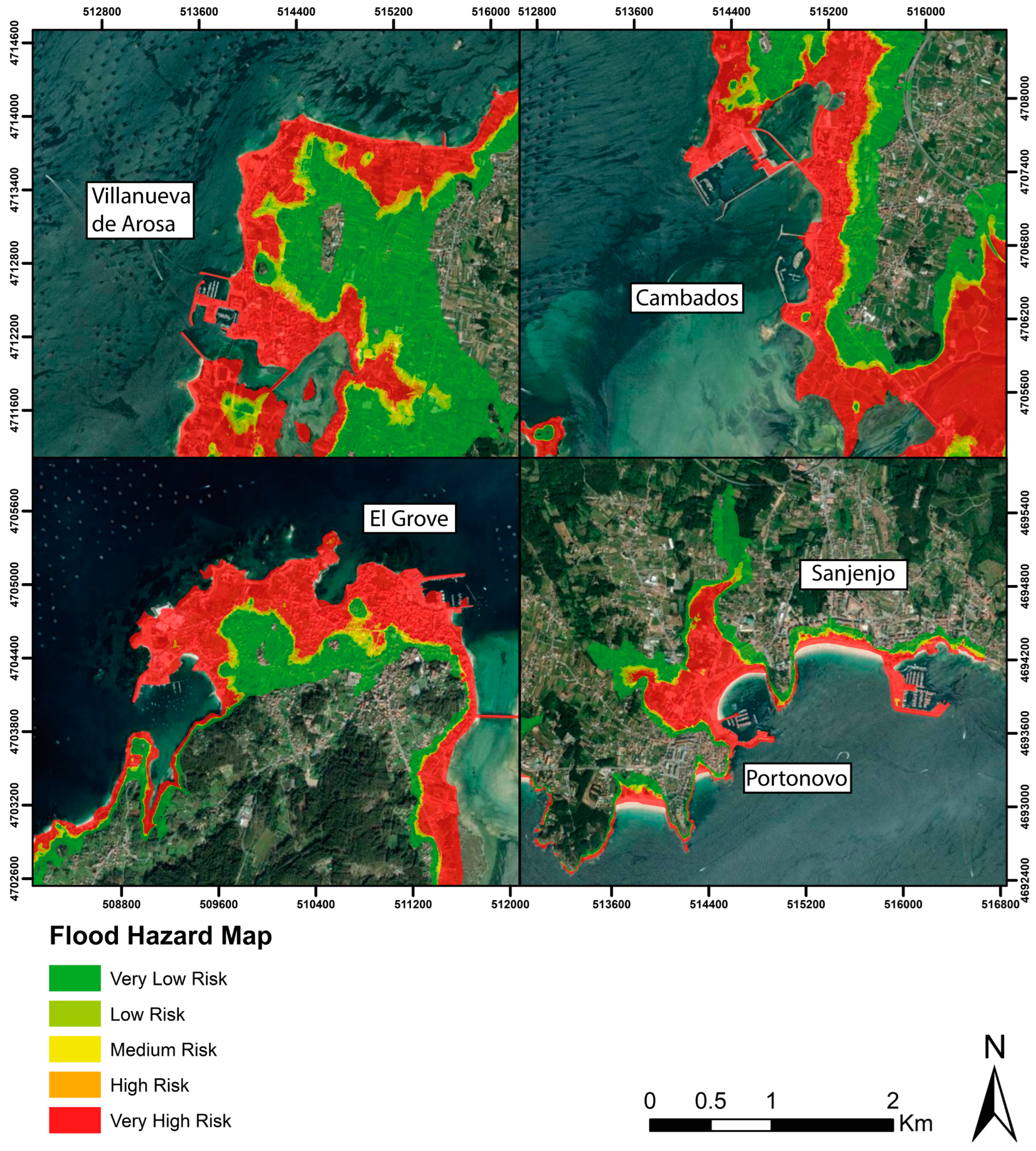
Creating detailed maps that focus on urban centers and urbanized areas in general allows for an examination of how different degrees of flood risk affect these zones (Figure 10). In this case, one can observe the urban centers of Villanueva de Arosa, Cambados, El Grove, and Sangenjo, which are areas with the highest population density (Table 2). These areas are also subject to the flood risk that encompasses the same zones explained previously.

Figure 10.
Detailed maps of the risk of flooding in the urban centers of each municipality.
Table 2.
Parameters for calculating exposure to flood risk (INE.es).
Using the flood risk map and the 2018 land use map, it is possible to assess exposure to risk by considering several parameters: municipality area, population size, population density, elevation, and distance from the coast of each municipality (Table 2). First, the urbanized areas, including urban centers, industrial areas, and infrastructure, can be identified using the land use map. Geographic information system (GIS) tools can be employed to delineate these areas and calculate the square kilometers of urbanized land. By applying geospatial techniques, the exposed area can be easily determined.
The results of flood risk exposure in the Ría of Arosa for different scenarios indicate that the coastal sector with the largest urbanized area exposed to the risk of marine flooding is 1.90 km2 in El Grove, where the population density is 494.46 inhabitants/km2, and the flood risk could potentially affect 944 people. However, the greatest population exposed to the risk is on the Isla de Arosa, where 947 people could be affected by flooding in an exposed urbanized area of 1.36 km2 (Figure 9B).
Summing up all the results, it is estimated that in the studied area of the Ría of Arosa, there is a total of 7.45 km2 of urbanized area exposed to the risk of flooding, putting 3707 inhabitants at risk. This represents approximately 6.46% of the total population in the studied area.
4. Discussion
4.1. Socio-Economic Impact Due to Coastal Flooding
Studying or assessing coastal vulnerability to the risk of sea-level rise-induced flooding in the Ría of Arosa coast, and considering that approximately 50% of the world’s population lives in the 10% of land area that comprises the coastline [40], it is possible to relate the results to the impact it will have on society and the economy of the study area.
In Spain, coastal population increased at an annual rate of 1.9% in the first decade of the 21st century. In Galicia specifically, the population density in municipalities located on the coast in the others provinces of Galicia (Coruña with 269 inhabitants/km2 and Lugo with 92 inhabitants/km2) is below the national average of Spain (435 inhabitants/km2). However, in the province of Pontevedra, the population density is higher, at 724 inhabitants/km2 [41]. The total population in coastal municipalities in Galicia is 1.1 million, with approximately 11,500 people living in flood-prone areas [42], meaning areas at high risk of flooding. In total, in Galicia, 59% of the total population of the autonomous community resides in its coastal areas, which account for less than 10% of the entire Galician territory [43].
Coastal tourism in Galicia, with more than 700 beaches along a 1400 km long coastline in northern Spain, is considered of great importance. The coastal areas of Rías Altas and Rías Bajas are the ones with the most coastal tourism activity, representing 53.7% of all coastal tourism in the autonomous community. In addition to coastal tourism, the Ría of Arosa is known for its significant wine tourism, featuring some of the best white wines in the country, as well as cultural tourism with visits to towns and churches (turismo.gal).
In Galicia, the majority of the employed population in coastal areas is in the service sector (financial, public, commercial, and tourism) (67.2%), and the primary sector activity in coastal areas, as mentioned earlier, includes fishing, shellfish harvesting, and aquaculture, with a high production and export of seafood products nationwide, particularly in aquaculture, which accounts for 98% of all mussel production in Spain [43].
Flooding in the area would have a significant negative impact on the economy, potentially affecting various sectors. In the tourism sector, flooding can lead to direct or indirect damage, causing harm to tourism infrastructure and significant losses for hotels and businesses dedicated to tourism. This disruption in business operations leads to reservation cancellations, reduced tourism, and significant income losses for tourism-related enterprises.
The loss of tourism can also occur due to tourists’ perceptions of risk and unfavorable conditions in the area. Decreased tourism results in reduced demand for personnel in the sector, leading to job losses for workers dependent on tourism, such as waiters, tour guides, hotel staff, etc. [44].
Another sector negatively affected by flood risk is the fishing and aquaculture industry, which can suffer damage to port and maritime infrastructure in addition to potential water contamination with sediments and harmful substances, leading to a decrease in marine density and biomass. This reduction in marine life results in decreased catches of fish and shellfish, reducing income for those engaged in these activities [45,46].
All these damages across various economic sectors generate costs for the recovery, repair, and reconstruction of the affected areas, requiring significant investments. This places pressure on the government and various organizations to allocate financial resources for damage repair, which can strain public finances and limit investment capacity in other areas [47].
4.2. Action Strategies against Coastal Flooding
In the face of the socio-economic impact that a coastal flooding event can cause, such as in the case of Ría of Arosa, it is crucial to develop and implement various strategies of action. These strategies can help minimize the damage caused by flooding and the associated repair costs. Currently, it is proposed that the most appropriate action is to carry out a combination of structural and non-structural measures, which are based on coastal territorial planning [48,49]. The preparation of these maps is above all useful to correctly establish territorial planning measures on the coast. In this work, different strategies focused on action against coastal flooding are presented.
One of the most commonly employed and potentially effective strategies in addressing the risk of coastal flooding involves coastal infrastructure, which can be divided into two types of defenses.
The first is hard engineering, which involves the construction and fortification of coastal structures (such as levees, breakwaters, groynes, and retaining walls). These measures can reduce the impact of the risk by mitigating wave intensity and coastal erosion, thus protecting populated areas and critical infrastructure. However, it is important to note that these measures may not be sustainable in the long term, as they can disrupt the natural physical environment, potentially altering the hydrodynamic regime.
The second is soft engineering, primarily focused on beach replenishment to protect areas experiencing sediment loss due to erosion. This approach aims to safeguard against extreme weather events, such as storms.
Another method that can be utilized is the restoration and management of coastal ecosystems like mangroves, wetlands, or marshes. These natural features can act as natural barriers against hazards, absorbing and retaining water [50,51].
Land use planning and urban development constitute another strategy against flood risk that can help reduce both damage and costs associated with natural events. This involves identifying high-risk zones and avoiding development in flood-prone areas, establishing buffer zones, and imposing construction restrictions in vulnerable areas. Promoting resilient construction practices in coastal regions is also crucial [51,52].
Passive strategies for mitigating flood risk include hazard response systems, early warning alerts, and community education and awareness. Hazard response and early warning systems entail monitoring and predicting sea levels, and disseminating clear information about flooding conditions and safety measures. This aids in predicting imminent flooding and the swift evacuation of populations in high-risk areas. Community education and awareness efforts involve providing information and promoting best safety practices, hazard response, and evacuation plans, as well as raising awareness about the importance of coastal systems [51,53].
5. Conclusions
After conducting the study, several conclusions can be drawn. Firstly, the methodology employed allows for the precise and effective delineation of coastal areas at risk of inundation due to sea-level rise at an economical cost. Furthermore, the results obtained provide valuable information regarding the degree of vulnerability and the flood risk profile along the southern coast of Ría of Arosa, in the event of a potential sea-level rise, whether it occurs gradually or during extreme events.
The vulnerability and flood risk maps represent the risk associated with any sea-level rise in Ría of Arosa. The calculated urbanized area affected by flood risk is approximately 7.45 km2, but this figure increases when considering agricultural areas and non-urbanized or uninhabited zones. Concerning the population exposed to flood risk, there is a total of 3707 individuals exposed, with a higher exposure on the Isle of Arosa and the El Grove peninsula.
The validity of the study’s methodology is confirmed through the alignment of the affected areas obtained in the results, using both the vulnerability index method (based on empirical parameters within the study area) and the risk method (based on deterministic methods employing temporal trend scenarios).
Lastly, the produced maps serve as a preventive measure that can help mitigate the risk of this coastline, which includes urban developments and tourism infrastructure, attracting a large number of tourists. Therefore, this tool can be effective in identifying sectors requiring structural measures to minimize the risk of sea-level rise impacts, whether due to natural trends or short- and long-term extreme events.
Author Contributions
Conceptualization, C.E.N., A.M.M.-G. and B.E.; methodology, C.E.N., A.M.M.-G. and B.E.; software, C.E.N. and B.E.; validation, C.E.N. and A.M.M.-G.; formal analysis, C.E.N., A.M.M.-G. and B.E.; investigation, C.E.N. and B.E.; resources, C.E.N., A.M.M.-G. and B.E.; data curation C.E.N., A.M.M.-G. and B.E.; writing—original draft preparation, C.E.N.; writing—review and editing, C.E.N. and A.M.M.-G.; visualization, C.E.N.; supervision, A.M.M.-G.; project administration, A.M.M.-G.; funding acquisition, A.M.M.-G. All authors have read and agreed to the published version of the manuscript.
Funding
Grant 131874B-I00 funded by MCIN/AEI/10.13039/501100011033. Ministry for the Ecological Transition and the Demographic Challenge.
Informed Consent Statement
Not applicable.
Data Availability Statement
The data presented in this study are available within this article.
Acknowledgments
This research was assisted by the GEAPAGE research group (Environmental Geomorphology and Geological Heritage) of the University of Salamanca.
Conflicts of Interest
The authors declare no conflict of interest.
References
- Park, S.J.; Lee, D.K. Prediction of coastal flooding risk under climate change impacts in South Korea using machine learning algorithms. Environ. Res. Lett. 2020, 15, 094052. [Google Scholar] [CrossRef]
- Kirschbaum, M.U. The temperature dependence of soil organic matter decomposition, and the effect of global warming on soil organic C storage. Soil Biol. Biochem. 2005, 27, 753–760. [Google Scholar] [CrossRef]
- Mori, N.; Yasuda, T.; Mase, H.; Tom, T.; Oku, Y. Projection of extreme wave climate change under global warming. Hydrol. Res. Lett. 2010, 4, 15–19. [Google Scholar] [CrossRef]
- Trenberth, K.E. Changes in precipitation with climate change. Clim. Res. 2011, 47, 123–138. [Google Scholar] [CrossRef]
- Rahmstorf, S. A semi-empirical approach to projecting future sea-level rise. Science 2007, 315, 368–370. [Google Scholar] [CrossRef]
- Intergovernmental Panel on Climate Change (IPCC). Climate Change 2007, The Physical Science Basis; Contribution of Working Group I to the Fourth Assessment Report of the Intergovernmental Panel on Climate Change 2007; Cambridge University Press: Cambridge, UK, 2007. [Google Scholar]
- Intragovernmental Panel on Climate Change (IPCC). Sea Level Change. In Climate Change 2013, The Physical Science Basis; Contribution of Working Group I to the Fifth Assessment Report of the Intergovernmental Panel on Climate Change 2013; Cambridge University Press: Cambridge, UK; New York, NY, USA, 2013. [Google Scholar]
- Intergovernmental Panel on Climate Change (IPCC). Climate Change 2014, Impacts, Adaptation, and Vulnerability; Part A: Global and Sectoral Aspects; Contribution of Working Group II to the Fifth Assessment Report of the IPCC 2014; Cambridge University Press: Cambridge, UK; New York, NY, USA, 2014; pp. 1–32. [Google Scholar]
- Vellinga, M.; Wood, R. Impacts of thermohaline circulation shutdown in the twenty-first century. Clim. Chang. 2008, 91, 43–63. [Google Scholar] [CrossRef]
- Pfeffer, W.T.; Harper, J.T.; O’Neel, S. Kinematic constraints on glacier contributions to 21st-century sea-level rise. Science 2008, 321, 1340–1343. [Google Scholar] [CrossRef]
- Grinsted, A.; Moore, J.C.; Jevrejeva, S. Reconstructing Sea level from paleo and projected temperatures 200–2100 AD. Clim. Dyn. 2010, 34, 461–472. [Google Scholar] [CrossRef]
- Vermeer, M.; Rahmstorf, S. Global Sea level linked to global temperature. Proc. Natl. Acad. Sci. USA 2009, 106, 21527–21532. [Google Scholar] [CrossRef]
- Katsman, C.A.G.; Oldenborgh, J.V. Exploring high-end scenarios for local sea level rise to develop flood protection strategies for a low-lying delta—The Netherlands as an example. Clim. Dyn. 2011, 109, 617–645. [Google Scholar] [CrossRef]
- Thieler, E.R.; Himmelstoss, E.A.; Zichichi, J.L.; Ergul, A. Digital Shoreline Analysis System (DSAS) Version 4.3—An ArcGIS Extension for Calculating Shoreline Change. In U.S. Geological Survey Open-File Report 2008–1278; U.S. Geological Survey: Reston, VA, USA, 2009. [Google Scholar]
- Ojeda, J.; Álvarez, J.I.; Martín, D.; Fraile, P. El uso de las TIG para el cálculo del índice de vulnerabilidad costera (CVI) ante una potencial subida del nivel del mar en la costa andaluza. GeoFocus Int. Rev. Geogr. Inf. Sci. Technol. 2009, 9, 83–100. [Google Scholar]
- Nicholls, R.J.; Cazenave, A. Sea-level rise and its impact on coastal zones. Science 2010, 328, 1517–1520. [Google Scholar] [CrossRef]
- Di Paola, G.; Rizzo, A.; Benassai, G.; Corrado, G.; Matano, F.; Aucelli, P.P.C. Sea-level rise impact and future scenarios of inundation riskalong the coastal plains in Campania (Italy). Environ. Earth Sci. 2021, 80, 608. [Google Scholar] [CrossRef]
- Bhable, S.; Kayte, S.; Mali, S.; Kayte, J.N.; Maher, R. A review paper on coastal hazard. Int. J. Eng. Res. Appl. 2015, 5, 83–93. [Google Scholar]
- Neumann, B.; Vafeidis, A.T.; Zimmermann, J.; Nicholls, R.J. Future coastal population growth and exposure to sea-leevl rise and coastal flooding-a global assessment. PLoS ONE 2015, 10, e0118571. [Google Scholar] [CrossRef] [PubMed]
- Klein, R.J.; Nicholls, R.J.; Ragoonaden, S.; Capobianco, M.; Aston, J.; Buckley, E.N. Technological options for adaptation to climate change in coastal zones. J. Coast. Res. 2001, 17, 531–543. [Google Scholar]
- Szlafsztein, C.; Sterr, H. A GIS-based vulnerability assessment of coastal natural hazards, state of Pará, Brazil. J. Coast. Conserv. 2007, 11, 53–66. [Google Scholar] [CrossRef]
- Balica, S.F.; Wright, N.G.; Van der Meulen, F. A flood vulnerability index for coastal cities and its use in assessing climate change impacts. Nat. Hazards 2012, 64, 73–105. [Google Scholar] [CrossRef]
- Vittal Hegde, A.; Radhakrishnan Reju, V. Development of coastal vulnerability index for Mangalore coast, India. J. Coast. Res. 2007, 23, 1106–1111. [Google Scholar] [CrossRef]
- Martínez-Graña, A.M.; Boski, T.; Goy, J.L.; Zazo, C.; Dabrio, C.J. Coastal-flood risk management in central Algarve: Vulnerability and flood risk indices (South Portugal). Ecol. Indic. 2016, 71, 302–316. [Google Scholar] [CrossRef]
- Martínez-Graña, A.; Gómez, D.; Santos-Francés, F.; Bardají, T.; Goy, J.L.; Zazo, C. Analysis of flood risk due to sea level rise in the Menor Sea (Murcia, Spain). Sustainability 2018, 10, 780. [Google Scholar] [CrossRef]
- Chazarra, A.; Flórez-García, E.; Peraza-Sánchez, B.; Tohá-Rebull, T.; Lorenzo-Mariño, B.; Criado, E.; Moreno-García, J.V.; Romero-Fresneda, R.; Botey, M.R. Mapas Climáticos de España (1981–2010) y Eto (1996–2016); Agencia Estatal de Meteorología (AEMET): Madrid, Spain, 2018.
- Martínez-Graña, A.M.; Goy, J.L.; Zazo, C. Cartografía Geomorfológica y Patrimonio Geológico Cuaternario en la Ría de Arosa (Pontevedra-La Coruña, Galice, España); Universidad Politécnica de Madrid: Madrid, Spain, 2007. [Google Scholar]
- Llana-Fúnez, S.; Marcos, A. The Malpica-Lamengo Line: A major crustal-scale shear zone in the Variscan belt of Iberia. J. Struct. Geol. 2001, 23, 1015–1030. [Google Scholar] [CrossRef]
- Cuesta, A. Petrología Granítica del Pluton de Caldas de Reyes (Pontevedra, España): Estructura, Mineralogía, Geoquímica y Petrogenesis; Nova Terra; Universidad de Oviedo: Oviedo, Spain, 1991; Volume 5, 363p. [Google Scholar]
- Gallastegui, G. Petrología del Macizo Granodiorítico de Bayo-Vigo (Provincia de Pontevedra, España). Ph.D. Thesis, Universidad de Oviedo, Oviedo, Spain, 1993; 363p. [Google Scholar]
- Pedraza, J. Geomorfología: Principios, Métodos y Aplicaciones; No. 551.4 PED; Rueda, 1996. Available online: https://www.researchgate.net/profile/Javier-De-Pedraza/publication/235864020_Geomorfologia_Principios_Metodos_y_Aplicaciones_Texto/links/5ebbb2bc299bf1c09ab944cf/Geomorfologia-Principios-Metodos-y-Aplicaciones-Texto.pdf (accessed on 10 October 2023).
- Martínez-Graña, A.M.; Arias, L.; Goy, J.L.; Zazo, C.; Silva, P. Geomorphology of the mouth of the Arosa estuary (Coruña-Pontevedra, Spain). J. Maps 2017, 13, 554–562. [Google Scholar] [CrossRef]
- Hallegatte, S. Strategies to adapt to an uncertain climate change. Glob. Environ. Chang. 2009, 19, 240–247. [Google Scholar] [CrossRef]
- Hammar-Klose, E.; Thieler, E.R. Coastal Vulnerability to Sea-Level Rise, a Preliminary Database for the US. Atlantic, Pacific, and Gulf of Mexico Coasts; Digital Data Series DDS-68; US Geological Survey: Reston, VA, USA, 2001; Volume 1.
- Pilkey, O.H.; Davis, T.W. An analysis of coastal recession models, North Carolina coast. In Sea-Level Fluctuation and Coastal Evolution; Nummedal, D., Pilkey, O.H., Howard, J.D., Eds.; SEPM (Society for Sedimentary Geology) Special Publications: Tulsa, OK, USA, 1987; Volume 41, pp. 59–68. [Google Scholar]
- Masselink, G.; Russell, P.; Rennie, A.; Brooks, S.; Spencer, T. Impacts of climate change on coastal geomorphology and coastal erosion relevant to the coastal and marine environment around the UK. MCCIP Sci. Rev. 2020, 2020, 158–189. [Google Scholar]
- Himmelstoss, E.A.; Henderson, R.E.; Kratzmann, M.G.; Farris, A.S. Digital Shoreline Analysis System (DSAS) Version 5.1 User Guide 2021–1091; US Geological Survey: Reston, VA, USA, 2021.
- Paleo, U.F. (Ed.) Incertidumbre en la tierra apacible. Los riesgos naturales en Galice. In Riesgos Naurales en Galice: El Encuentro Entre Naturales y Sociedad; Servizo de Publicacións e Intercambio Científico da USC: Santiago de Compostela, Spain, 2010; pp. 1–9. [Google Scholar]
- Luque, L.; Lario, J.; Civis, J.; Silva, P.G.; Zazo, C.; Goy, J.L.; Dabrio, J. Sedimentary record of a tsunami during Roman times, Bay of Cadiz, Spain. J. Quat. Sci. 2002, 17, 623–631. [Google Scholar] [CrossRef]
- Shi, C.; Hutchinson, S.M.; Yu, L.; Xu, S. Towards a sustainable coast: An integrated coastal zone management framework for Shanghai, People's Republic of China. Ocean. Coast. Manag. 2001, 44, 411–427. [Google Scholar] [CrossRef]
- Toubes, D.R.; Gössling, S.; Hall, C.M.; Scott, D. Vulnerability of coastal beach tourism to flooding: A case study of Galice, Spain. Environments 2017, 4, 83. [Google Scholar] [CrossRef]
- De Galice, A. Estudio Ambiental Estratégico. Plan de Xestión do Risco de Inundación da Demarcación. In Hidrográfica de Galice-Costa (Ciclo 2015–2021); Aguas de Galice 2016; Santiago de Compostela, Spain, 2016; Available online: https://www.miteco.gob.es/es/agua/temas/gestion-de-los-riesgos-de-inundacion/planes-gestion-riesgos-inundacion/evaluacion_ambiental_planes_gestion_ri.html (accessed on 10 October 2023).
- Ferreiro, F.J.; Vaquero, A. Análisis económico del litoral gallego: Situación actual y perspectivas futuras. Adm. Ciudad. 2010, 5, 47–66. [Google Scholar]
- Toubes, D.R.; Araújo-Vila, N.; Fraiz-Bera, J.A. Factors influencing the assessment of tourism damage caused by river floods. Rev. Tur. Desenvolv. 2021, 1, 51–61. [Google Scholar]
- Milner, A.M.; Robertson, A.L.; McDermott, M.J.; Klaar, M.J.; Brown, L.E. Major flood disturbance alters river ecosystem evolution. Nat. Clim. Chang. 2012, 3, 137–141. [Google Scholar] [CrossRef]
- George, S.D.; Baldigo, B.P.; Smith, A.J.; Robinson, G.R. Effects of extreme floods on trout populations and fish communities in a Catskill Mountain River. Freshw. Biol. 2015, 60, 2511–2522. [Google Scholar] [CrossRef]
- Adger, W.N.; Hughes, T.P.; Folke, C.; Carpenter, S.R.; Rockstrom, J. Social-ecological resilience to coastal disasters. Science 2005, 309, 1036–1039. [Google Scholar] [CrossRef]
- Malekpour, S.; Brown, R.R.; de Haan, F.J.; Wong, T.H.F. Preparing for Disruptions: A Diagnostic Strategic Planning Interpretation for Sustainable Development. Cites 2017, 63, 58–69. [Google Scholar] [CrossRef]
- Dedekorkut-Howes, A.; Torabi, E.; Howes, M. When the tide gets high: A review of adaptative responses to sea level rise and coastal flooding. J. Environ. Plan. Manag. 2020, 63, 2102–2143. [Google Scholar] [CrossRef]
- Temmerman, S.; Meire, P.; Bouma, T.J.; Herman, P.M.; Ysebaert, T.; De Vriend, H.J. Ecosystem-based coastal defence in the face of global change. Nature 2013, 504, 79–83. [Google Scholar] [CrossRef]
- Anfuso, G.; Postacchini, M.; Di Luccio, D.; Benassai, G. Coastal sensitivity/vulnerability characterization and adaptation strategies: A review. J. Mar. Sci. Eng. 2021, 9, 72. [Google Scholar] [CrossRef]
- Bapalu, G.V.; Sinha, R. GIS in flood hazard mapping: A case study of Kosi River Basin, India. GIS Dev. Wkly. 2005, 1, 1–3. [Google Scholar]
- Di Luccio, D.; Benassai, G.; Budillon, G.; Mucerino, L.; Montella, R.; Pugliese Carratelli, E. Wave run-up prediction and observation in a micro-tidal beach. Nat. Hazards Earth Syst. Sci. 2018, 18, 2841–2857. [Google Scholar] [CrossRef]

Disclaimer/Publisher’s Note: The statements, opinions and data contained in all publications are solely those of the individual author(s) and contributor(s) and not of MDPI and/or the editor(s). MDPI and/or the editor(s) disclaim responsibility for any injury to people or property resulting from any ideas, methods, instructions or products referred to in the content. |
© 2023 by the authors. Licensee MDPI, Basel, Switzerland. This article is an open access article distributed under the terms and conditions of the Creative Commons Attribution (CC BY) license (https://creativecommons.org/licenses/by/4.0/).