Article

Research on a Decoupling Algorithm for the Dual-Deformable-Mirrors Correction System

1
Faculty of Automation and Information Engineering, Xi’an University of Technology, Xi’an 710048, China
2
Shaanxi Civil-Military Integration Key Laboratory of Intelligence Collaborative Networks, Xi’an 710126, China
3
College of Physics and Electronics, Shaanxi University of Technology, Hanzhong 723001, China
*
Author to whom correspondence should be addressed.
Appl. Sci. 2023, 13(22), 12112; https://doi.org/10.3390/app132212112
Submission received: 1 October 2023 / Revised: 29 October 2023 / Accepted: 2 November 2023 / Published: 7 November 2023

Abstract

:
Wavefront distortion caused by atmospheric turbulence can be described as different types of aberrations, such as piston, tilt, defocusing, astigmatism, coma and so on. The operation of dual deformable mirrors can have mutual coupling effects, which affect the correction effect of wavefront distortion. This study combines a fast-steering mirror (FSM) and a deformable mirror (DM) to form a dual-deformable-mirrors wavefront correction system, and proposes a decoupling algorithm that can correct any specified aberration. In this decoupling algorithm, both the FSM and the DM are controlled using the mode method, and the specific corrected aberrations are obtained based on a limited matrix. The compensation ability of the DM is directly characterized by the mode coefficients of the aberrations, which can achieve independent correction of any order of aberrations and effectively reduce the coupling effect of the dual-deformable-mirrors wavefront correction system. An adaptive optical dual-deformable-mirrors wavefront correction system experiment was built to verify the decoupling algorithm. When the DM corrects the 3rd-, 10th-, and 25th-order aberrations, and the FSM only corrects the 1st- and 2nd-order aberrations, the coupling coefficients are approximately 1.17 × 1 0 3 , 1.814 × 1 0 2 and 7.81 × 1 0 3 , respectively, and their magnitude reaches 10−2 and below 10−2, respectively. The experimental results show that the decoupling algorithm can effectively suppress the coupling effect between the FSM and the DM.

1. Introduction

The Woofer–Tweeter system is a typical dual-deformable-mirrors wavefront correction system [1], consisting of a large stroke, low spatial-frequency deformable mirror (Woofer), and a small stroke, high spatial-frequency deformable mirror (Tweeter). These two deformable mirrors work together to improve the wavefront correction effect. However, when both deformable mirrors are working simultaneously, coupling effects occur, which can lead to the wastage of correction ability by some deformable mirrors. If this phenomenon cannot be effectively suppressed, coupling errors will gradually accumulate, eventually leading to the complete consumption of the stroke of the deformable mirror by coupling. When the aberration to be corrected in the system changes, the deformable mirror affected by coupling will have difficulty in effectively compensating for the aberration, leading to a decrease in the system’s correction ability [2]. Therefore, coupling compensation between deformable mirrors has become an important research direction for dual-deformable-mirrors wavefront correction systems in terms of aberration compensation ability and stability.
To fully utilize the advantages of adaptive optics dual-deformable-mirrors wavefront correction systems, it is crucial to further improve their performance and eliminate potential coupling between the deformable mirrors. Numerous scholars have addressed this issue, with different approaches proposed over the years. In 1998, Sivokon analyzed combining low and high spatial-resolution systems to enhance their spatial correction capability, but this approach required two expensive adaptive optical systems [3]. In 2013, Liu proposed a decoupling control algorithm based on Zernike mode decomposition that greatly reduced costs but could not independently correct high-order aberrations [4]. In 2016, Liu proposed a Zonal decoupling algorithm that utilizes the traditional direct slope method to control both deformable mirrors [5]. This approach effectively suppressed the coupling effect between the deformable mirrors, but was not suitable for engineering applications [2]. In 2018, Cheng proposed a slope-based decoupling algorithm that showed better performance in suppressing coupling errors but was also unsuitable for dual-deformable-mirrors wavefront correction systems with FSM and DM combined [6]. In 2021, Kong introduced a decoupling control algorithm based on Numerical Orthogonal Polynomials (NOP), which aimed to eliminate cross coupling between dual wavefront correctors. However, the limitation of this algorithm is that each order of aberration cannot be independently corrected [7]. In 2021, Yang used dual-deformable-mirrors combination control for fiber power coupling, enhancing the efficiency of spatial optical fiber coupling [8]. In 2023, Liu proposed a dual-deformable-mirrors decoupling control method based on pattern projection suppression that enabled the two deformable mirrors to work efficiently together while eliminating low-order correction components in Tweeter [9]. These decoupling algorithms have been successfully applied to various adaptive optical dual-deformable-mirrors wavefront correction systems, significantly reducing coupling effects between deformable mirrors. Nonetheless, few decoupling algorithms are available for dual-deformable-mirrors wavefront correction systems combined with FSM and DM, where each order of aberration cannot be independently controlled or corrected. Different application scenarios have varying requirements for different types of aberrations. Hence, specific aberrations can be corrected according to actual needs to meet the diverse needs of different application scenarios, improving system performance and laying the foundation for large aperture telescope application. In the field of astronomical observation, as the aperture of telescopes continues to increase, so does their sensitivity to atmospheric turbulence. This results in larger amplitude and higher spatial-resolution wavefront aberrations that need to be corrected. Therefore, adaptive optical systems must also increase their ability to correct these aberrations with greater accuracy and amplitude. However, different types of wavefront correctors are often limited by technical issues such as material selection, manufacturing processes, and system-integration complexity. As a result, it becomes challenging for adaptive optical systems equipped with a single wavefront corrector to meet the requirements of large travel and high spatial-frequency aberrations.
To address this challenge, researchers have explored the use of multiple wavefront correctors with different performance characteristics working together. By combining the characteristics of each corrector, it is possible to achieve high amplitude correction for low spatial-frequency aberrations and synchronous correction for small amplitude high spatial-frequency aberrations. This cooperative approach has proven to be an effective solution to the limitations faced by single wavefront correctors in adaptive optical systems. This article proposes a decoupling algorithm to address the issues associated with coupling between FSM and DM in dual-deformable-mirrors wavefront correction systems. The decoupling algorithm utilizes the mode method to control FSM and DM. By applying the mode method wavefront reconstruction principle, the slope measured by the Hartmann wavefront sensor is converted into Zernike coefficients, which are then used to directly calculate the initial control voltage for the FSM and DM. The final control voltage of the FSM and DM is then determined using a Proportional Integral (PI) controller, enabling independent correction of any order aberration while avoiding cross-coupling effects. This approach significantly improves the performance and flexibility of the system, making it of great significance for enhancing their capabilities.
The rest of this paper is organized as follows. Section 2 describes the principle of the dual-deformable-mirrors wavefront correction system and decoupling algorithm. Section 3 conducts a numerical simulation of the proposed algorithm. Section 4 establishes an experimental platform for the dual-deformable-mirrors wavefront correction system for experimental research. Section 5 provides a detailed analysis of the coupling effect. Finally, Section 6 concludes the paper.

2. Principle of Wavefront Correction with Dual Deformable Mirrors

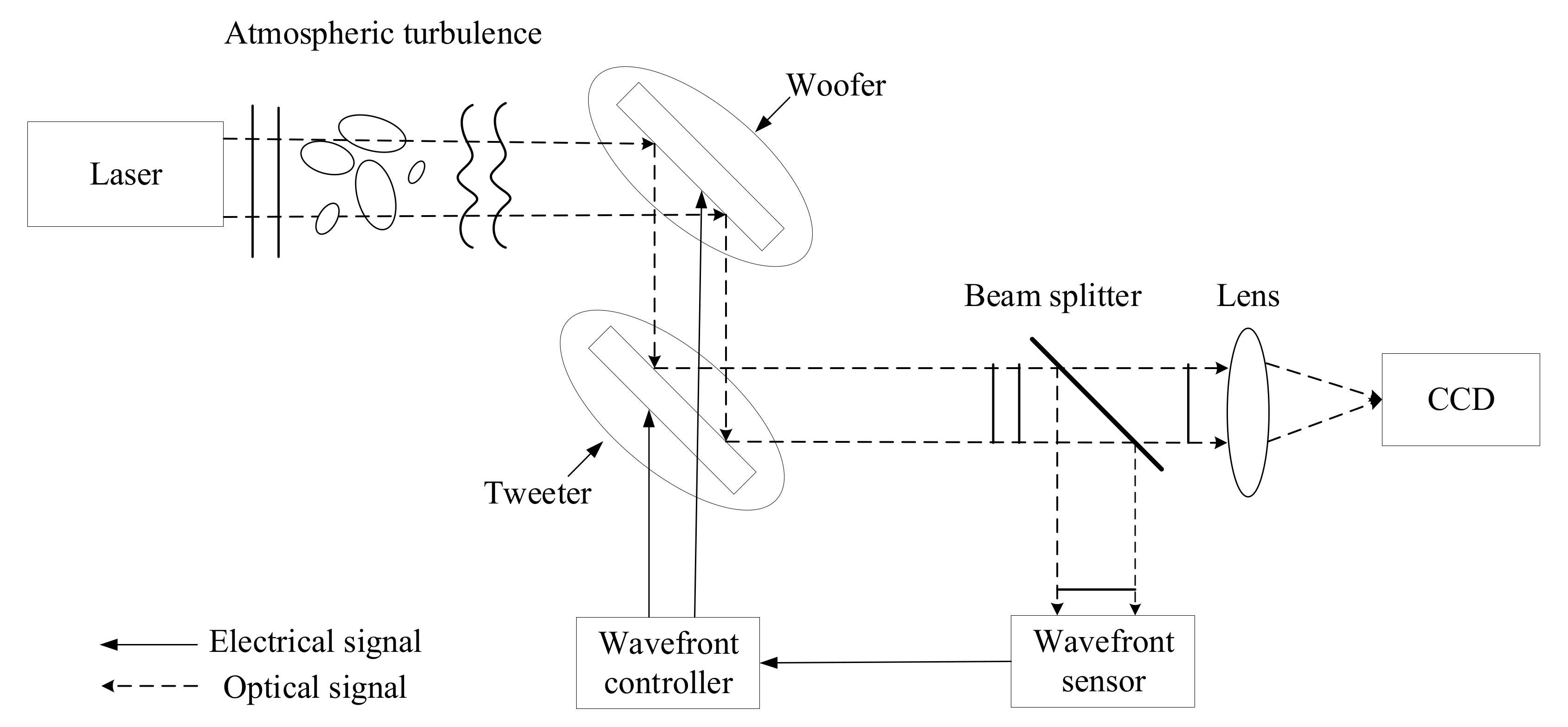
2.1. Principle of Dual-Deformable-Mirrors Correction System

The working principle of the dual-deformable-mirrors correction system is shown in Figure 1. The system mainly consists of three parts: wavefront sensor, wavefront controller, and wavefront corrector (two) [10]. When a beam of light propagates in the atmosphere, wavefront distortion is generated due to atmospheric turbulence, and it is corrected using a wavefront corrector. In the dual-deformable-mirrors correction system of this study, wavefront distortion is graded and corrected by two wavefront correctors. Wavefront corrector 1 is generally an FSM or a large stroke, low spatial-frequency DM (commonly referred to as Woofer), responsible for correcting low-order aberrations. Wavefront corrector 2 is generally a small stroke, high spatial-frequency DM (commonly referred to as Tweeter), responsible for correcting high-order aberrations. The system utilizes wavefront sensors to measure the wavefront of the received beam in real-time, feedback the measured wavefront information to the wavefront controller, and then calculate and obtain the control voltage of the wavefront corrector through a certain control algorithm, providing real-time control signals for the wavefront corrector. The wavefront corrector receives real-time control voltage from the wavefront controller, fits the surface shape to correct wavefront distortion, and improves the communication quality of the dual-deformable-mirrors wavefront correction system.

2.2. Principle of Separation Coefficient Algorithm

The distorted wavefront generated by the interference of atmospheric turbulence can be expanded using Zernike polynomials, and the expression for wavefront ϕ ρ is [11,12]:
ϕ ρ = i = 1 a i Z i ρ
In the equation, a i represents the i-th order Zernike coefficient and Z i ρ represents the i-th order Zernike polynomial [12]. This study uses the Zernike polynomial defined by Noll in polar coordinates, whose expression is [13]:
Z   i = n + 1 R n m ρ 2 cos m θ m 0   a n d   m   i s   e v e n n + 1 R n m ρ 2 sin m θ m 0   a n d   m   i s   o d d n + 1 R n m ρ m = 0
Among them, (ρ, θ) is the polar coordinate. The integers m and n represent the angular and radial levels, respectively, and there is a relationship between the two as follows:
m n n m = k k N
And the radial polynomial R n m ρ is defined as [14]:
R n m ρ = s = 0 n m 2 1 s n s ! s ! n + m / 2 s ! n m / 2 s ! ρ n 2 s
The lower-order modes of Zernike polynomials in the circular domain are consistent with Seidel aberrations, and the specific expressions for the aberrations represented by the first 15 orders of Zernike polynomials are shown in Table 1.
Assuming the influence function of the i-th actuator of the DM is fi, it can generally be measured using a Zygo interferometer or wavefront sensor. The j-th order Zernike mode is denoted as Zj. The cross-correlation matrix Cfz between the influence function of the DM and the Zernike modes can be represented as [9]:
C f z i , j = f i r Z j r d 2 r
Similarly, the expression for calculating the autocorrelation matrix Cff between the influence functions of the DM actuator is as follows [9]:
C f f i , j = f i r f j r d 2 r
According to Equations (5) and (6), the conversion matrix T from the Zernike mode coefficient to the control voltage of the DM can be obtained as [9]:
T = C f f i , j 1 C f z i , j
In the equation, Cfz is the cross-correlation matrix obtained from Equation (5). Cff is the autocorrelation matrix obtained from Equation (6). C f f 1 is the inverse matrix of matrix Cff; then, the expression of the control voltage to be loaded each time by the DM is [9]:
v = T a
In the equation, a = a 1 , a 2 , ... , a n T is the Zernike coefficient, dimension is n × 1 , and n is the order of the Zernike polynomial. T is the transformation matrix between Zernike mode coefficients and DM control voltages. v = v 1 , v 2 , ... , v P T is the initial control voltage of the DM, and P is the number of actuators of the DM.
The Shack–Hartmann Wavefront Sensor (SH-WFS) can measure the slope, and its slope matrix is represented as:
S   =   Z a
In the equation, S = S x 1 , S x 2 , ... , S x m , S y 1 , S y 2 , ... , S y m is the slope matrix directly measured by the SH-WFS, dimension is 2 m × 1 , and m is the number of subapertures of the SH-WFS. Z is the wavefront reconstruction matrix, dimension is 2 m × n . a = a 1 , a 2 , ... , a n T is the Zernike coefficient, dimension is n × 1 , and n represents the order of the Zernike polynomial.
According to the wavefront reconstruction principle of the Zernike mode method [15], the Zernike coefficient can be reconstructed using the measured slope S, and the expression is as follows:
a = Z + S
In the equation, Z+ is the generalized inverse matrix of Z.
The mode coefficient expression for correcting aberrations with Woofer is as follows:
a w = I w a = I w Z + S
In the equation, a w = a w 1 , a w 2 , ... , a w n T is the mode coefficient assigned to the Woofer for aberration correction. Iw is the diagonal matrix of n × n , also known as the limiting matrix of low-order aberrations. For example, if the Woofer corrects 1st- to 2nd-order aberrations, the expression for Iw is as follows:
I w = 1 1 0 ... 0 0
Based on Equation (8), the initial control voltage of the Woofer can be directly calculated. The expression is:
v w = T w a w = T w I w Z + S
In the equation, v w = v w 1 , v w 2 , ... , v w h T is the initial control voltage of the Woofer, and h is the number of actuators for the Woofer. Tw is the conversion matrix between the Zernike mode coefficient and the control voltage of the Woofer, calculated by Equations (5)–(7). a w is the mode coefficient that the Woofer calculated by Equation (11) will correct for aberrations.
After obtaining the initial control voltage of the Woofer using Equation (13), a PI controller is used to solve the final control voltage of the Woofer and send it to the Woofer for operation. In order to accurately calculate the control voltage of the Woofer, the final control voltage expression of the Woofer at time k is:
V w ( k ) = k i _ w V w ( k 1 ) + k p _ w v w ( k 1 )
In the equation, k i _ w is the integral gain coefficient of the PI controller, and k p _ w is the proportional gain coefficient of the PI controller. V w ( k ) = V w 1 , V w 2 , V w 3 , ... , V w h T is the final control voltage of the Woofer, and h is the number of actuators for the Woofer. v w ( k 1 ) is the initial control voltage of the Woofer calculated at the previous moment.
At the same time, the mode coefficient expression for correcting aberrations in Tweeter is as follows:
a t = I t a = I t Z + S
In the equation, a t = a t 1 , a t 2 , ... , a t n T is the mode coefficient assigned to Tweeter for aberration correction. It is the diagonal matrix of n × n , also called the limiting matrix of higher-order aberrations. For example, if Tweeter only corrects 3rd-order aberrations, the expression for It is as follows:
I t = 0 0 1 ... 0 0
According to Equation (8), the initial control voltage of the Tweeter can be directly calculated, and its expression is:
v t = T t a t = T t I t Z + S
In the equation, v t = v t 1 , v t 2 , ... , v t t T is the initial control voltage of the Tweeter, and t is the number of actuators for the Tweeter. Tt is the conversion matrix between Zernike mode coefficient and the Tweeter control voltage, calculated by Equations (5)–(7). a t is the mode coefficient of the Tweeter calculated by Equation (15) that will correct for aberrations.
After obtaining the initial control voltage of the Tweeter using Equation (17), a PI controller is used to solve the final control voltage of the Tweeter and send it to the Tweeter for operation. In order to accurately calculate the control voltage of the Tweeter, the final control voltage expression of the Tweeter at time k is:
V t ( k ) = k i _ t V t ( k 1 ) + k p _ t v t ( k 1 )
In the equation, k i _ t is the integral gain coefficient of the PI controller, and k p _ t is the proportional gain coefficient of the PI controller. V t ( k ) = V t 1 , V t 2 , V t 3 , ... , V t t T is the final control voltage of the Tweeter, and t is the number of actuators for the Tweeter. v t k 1 is the initial control voltage of the Tweeter calculated at the previous moment.
By using Equations (14) and (18), the final control voltage of the Woofer and the Tweeter can be calculated to obtain the corrected wavefront phase. The corrected wavefront phase is denoted as ϕ k , and the iterative phase expression after the k-th correction is:
ϕ k + 1 = ϕ k + ( V w k f w ) + ( V t k f t )
In the equation, fw is the influence function of the Woofer, and ft is the influence function of the Tweeter.
In practical applications, the measurement and calculation of Z, Z+, Tw, Tt, fw and ft can be completed in advance and saved for future use, allowing for quick and efficient access during the calibration process. This decoupling algorithm not only streamlines the program’s performance by reducing its running time and storage space but also significantly enhances computational efficiency. This decoupling algorithm provides the flexibility to correct any order of aberration independently, while also enabling independent correction of each order of aberration. This makes it highly adaptable to different types of dual-deformable-mirrors system and enables efficient and accurate wavefront correction for a wide range of applications.
The above elucidates the principle of the separation coefficient algorithm, and the flowchart of the algorithm is illustrated in Figure 2. The algorithm proposed in this article is implemented using MatlabR2016b software. The process begins by setting the slope data Sr of the ideal wavefront to a 0 matrix, representing a plane wavefront. The slope data collected by the Hartmann wavefront sensor, Sc, is then subtracted from Sr to obtain the error slope Se. Using the wavefront reconstruction principle, Se is converted into Zernike coefficients, which are then used to calculate the Zernike coefficients that need to be corrected by FSM and DM. A limited matrix is used for this purpose. Next, the initial voltage is calculated based on its conversion matrix. The voltage at the previous moment is used to solve the voltage of FSM and DM at the previous moment. The PI controller is employed to determine the final control voltage for both FSM and DM. These voltages are then used to drive the FSM and DM, obtaining the corrected residual wavefront correction. The Hartmann wavefront sensor can then obtain the slope data of the corrected residual wavefront, forming a closed-loop correction.
The Peak-to-Valley (PV) value represents the difference between the maximum and minimum values of the wavefront phase, indicating the maximum level of wavefront phase defects. However, it ignores the proportion of this part in the overall wavefront. Therefore, evaluating wavefront quality based solely on PV value is not rigorous enough. On the other hand, the Root-Mean-Square (RMS) value focuses more on the overall information of the wavefront phase. It reflects the degree of deviation of all points on the wavefront from their ideal positions. Therefore, combining PV and RMS values can more accurately represent the wavefront condition. This study mainly uses PV and RMS values to evaluate the level of distortion in the wavefront [16]. Based on the phase compensation of two deformable mirrors, the coupling coefficient is used to quantitatively describe the coupling effect of the adaptive optics dual-deformable-mirrors correction system [4]. A coupling coefficient value closer to 0 indicates a smaller coupling effect between Woofer and Tweeter, while a coupling coefficient value closer to 1 indicates a larger coupling effect.

3. Numerical Simulation Analysis

To further validate the algorithm proposed in this article, experimental data were analyzed in the laboratory of Xi’an University of Technology. The transmitting end of the data measurement was positioned in Teaching building 5 of Xi’an University of Technology, while the receiving end was located in building 2 of Discipline, and the straight-line distance between the two buildings is 600 m. The slope data of wavefront distortion were measured using the Shack–Hartmann wavefront sensor. According to the wavefront reconstruction principle [15], the wavefront reconstruction matrix was inverted and the product of the slope data measured by the Hartmann wavefront sensor was obtained (i.e., Equation (10) to obtain the initial Zernike coefficient of wavefront distortion, as depicted in Figure 3a. Given the Zernike coefficient value of wavefront distortion, the phase of wavefront distortion can be calculated by substituting it into Equation (1), as shown in Figure 3b, which displays the phase diagram of wavefront distortion.
Next, a dual-deformable-mirrors wavefront correction system consisting of FSM (Woofer) and a 69-unit DM (Tweeter) is mainly used to correct the wavefront distortion data measured in the experiment. The FSM corrects the 2nd-order aberration, the DM corrects the 30th-order aberration, and the parameters of the PI controller are set to: k i _ w = 0.999 , k p _ w = 0.1 , k i _ t = 0.999 , k p _ t = 0.1 . The wavefront phase diagrams corrected by the FSM and DM, respectively, as well as the wavefront phase diagrams corrected by working together, are shown in Figure 4.
Figure 4 presents the phase diagrams of the FSM and DM after correcting the aberration individually and in combination. Specifically, Figure 4a illustrates the wavefront phase diagram after correction with an FSM, while Figure 4b shows the residual wavefront phase diagram after correction with a DM. Additionally, Figure 4c depicts the residual wavefront phase diagram after both FSM and DM have been employed for correction. As shown in Figure 3a, the 2nd order and 30th-order aberrations have the largest Zernike coefficient values, indicating that they contribute significantly to the total wavefront aberration. Therefore, the FSM is used to correct the 2nd-order aberration, while the DM corrects the 30th-order aberration. Comparing Figure 3b with Figure 4b, it is evident that the tilted degree of the corrected wavefront distortion phase diagram is minimal, indicating that the residual wavefront after correction has a minimal proportion of tilted aberrations. However, when the DM was used to correct the 30th-order aberration without compensating for the 2nd-order aberration, as shown in Figure 4b, there was a degree of tilt in the corrected wavefront phase diagram. As seen in Figure 4c, there was a significant change between the corrected wavefront phase diagram and the initial distorted wavefront phase diagram. By evaluating their PV and RMS values, it can be concluded that the proposed algorithm’s wavefront correction ability is accurately reflected, demonstrating that the decoupling algorithm achieves independent correction of specified aberrations.
In a dual-deformable-mirrors wavefront correction system, the deformation generated by two deformable mirrors is typically used to correct wavefront aberration. However, when the two deformable mirrors are coupled, their deformations can affect each other, leading to an unwanted coupling effect. To evaluate this effect, the coupling coefficient is employed as an important indicator. Based on the influence function and control voltage of the FSM and DM, the correction amount of the FSM and DM is calculated. Substituting these correction amounts into the coupling coefficient expression [4], the value of the coupling coefficient between the FSM and DM is solved. The coupling coefficient diagram is presented in Figure 5, where the black line represents the coupling coefficient curve for 2nd-order aberrations corrected by the FSM, and 2nd-order and 30th-order aberrations corrected by the DM. It is observed that there exists a coupling effect between the FSM and DM with a coupling coefficient of approximately 4.8 × 1 0 1 , indicating an order of approximately 10−1. In the proposed algorithm, a finite matrix is used to constrain the Zernike coefficients. By modifying the elements on the diagonal of the matrix defined by Equations (12) and (16), it is ensured that only the 2nd-order aberration is corrected by the FSM, while only the 30th-order aberration is corrected by the DM. As shown in the red line, this results in a coupling coefficient value around 1.3 × 1 0 2 , indicating that the algorithm effectively suppresses the coupling effect between the FSM and DM.

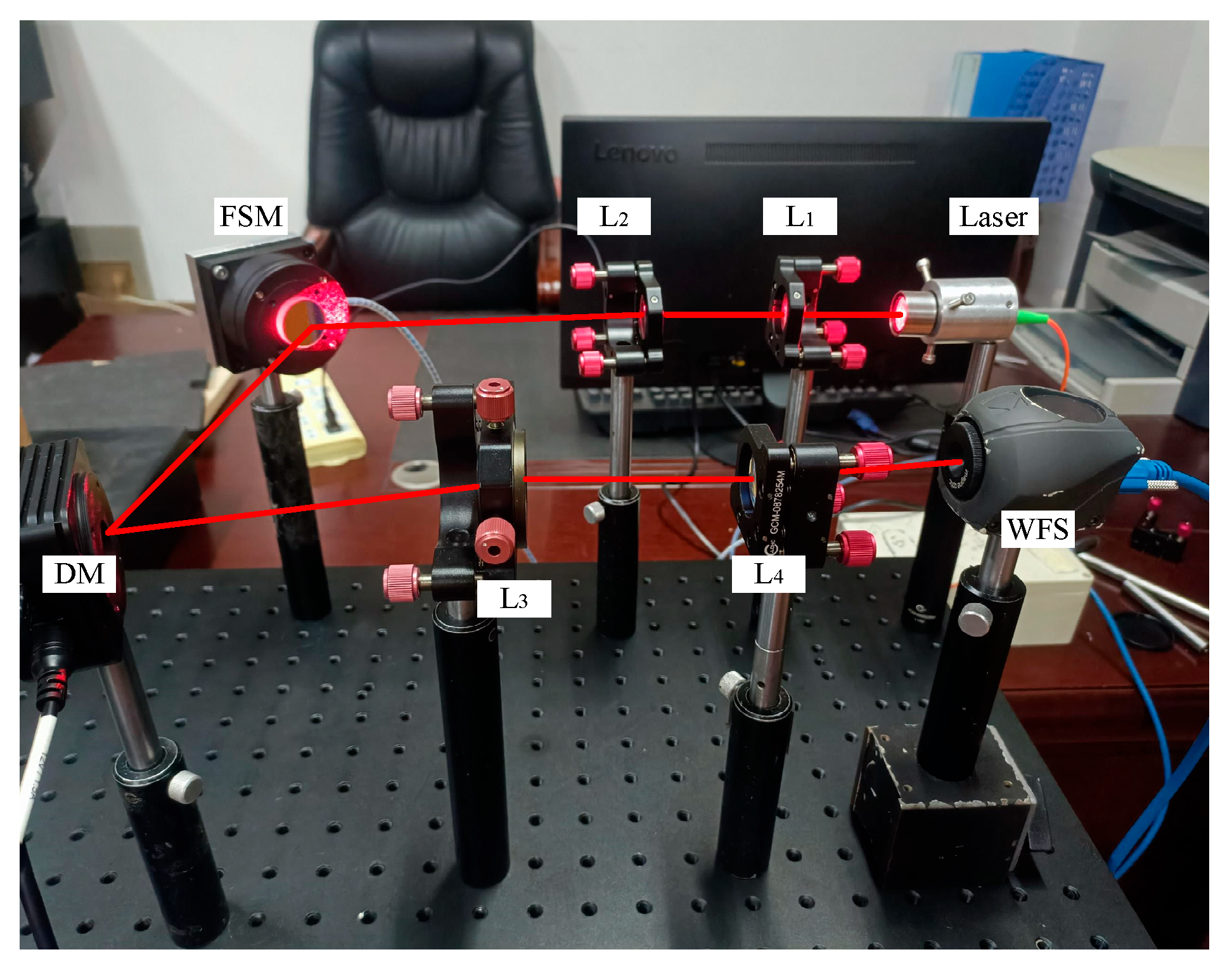
4. Experimental Research

In adaptive optics systems, the FSM is usually regarded as a special DM that only produces tilt aberration compensation. To verify the importance of theoretical results, an experimental platform for a dual-deformable-mirror wavefront correction system was built indoors to correct wavefront distortion. The experimental setup is illustrated in Figure 6. The beam is emitted by a 650 nm semiconductor laser and extended and collimated through a 4f system composed of lens L1 and lens L2. The collimated beam is incident on the surface of the FSM, and then on the surface of the DM. The FSM and DM correct the specified aberrations as needed. The beam corrected by FSM and DM is incident onto a 4f system composed of lens L3 and lens L4 for beam reduction. The wavefront sensor detects at the focal point of lens L4 and transmits the detected wavefront information to the wavefront controller (computer). The computer calculates the control voltage using an appropriate control algorithm and sends it to the FSM and DM for closed-loop correction of the distorted wavefront over multiple iterations. This forms a typical adaptive optics dual-deformable-mirrors closed-loop correction system.
According to the experimental diagram constructed in Figure 6, the experimental parameters of the PI controller are: k i _ w = 0.999 , k p _ w = 0.1 , k i _ t = 0.999 , k p _ t = 0.1 , and the decoupling algorithm studied in this paper is used for indoor experiments. Figure 7 shows the coupling coefficient curve between the FSM and the DM.
Figure 7a presents the coupling coefficient curve when the FSM only corrects the 1st and 2nd-order aberrations, and the DM only corrects the 3rd-order aberrations. The approximate trend of the curve indicates that the coupling coefficient is approximately 1.17 × 1 0 3 . Figure 7b displays the coupling coefficient curve when the FSM only corrects the 1st and 2nd-order aberrations, and the DM only corrects the 10th order aberrations, with a coupling coefficient of approximately 1.814 × 1 0 2 . Figure 7c shows the coupling coefficient curve when the FSM only corrects the 1st- and 2nd- order aberrations, and the DM only corrects the 25th-order aberrations, with a coupling coefficient of approximately 7.81 × 1 0 3 . Through experiments, it was demonstrated that the decoupling algorithm is effective in suppressing the coupling effect between the FSM and the DM. It can perform graded correction on aberrations, selectively allocate any order of aberrations for correction, and achieve independent correction of any order of aberrations. The coupling coefficients reached levels of 10−2 and below, effectively suppressing the coupling effect between the FSM and the DM.

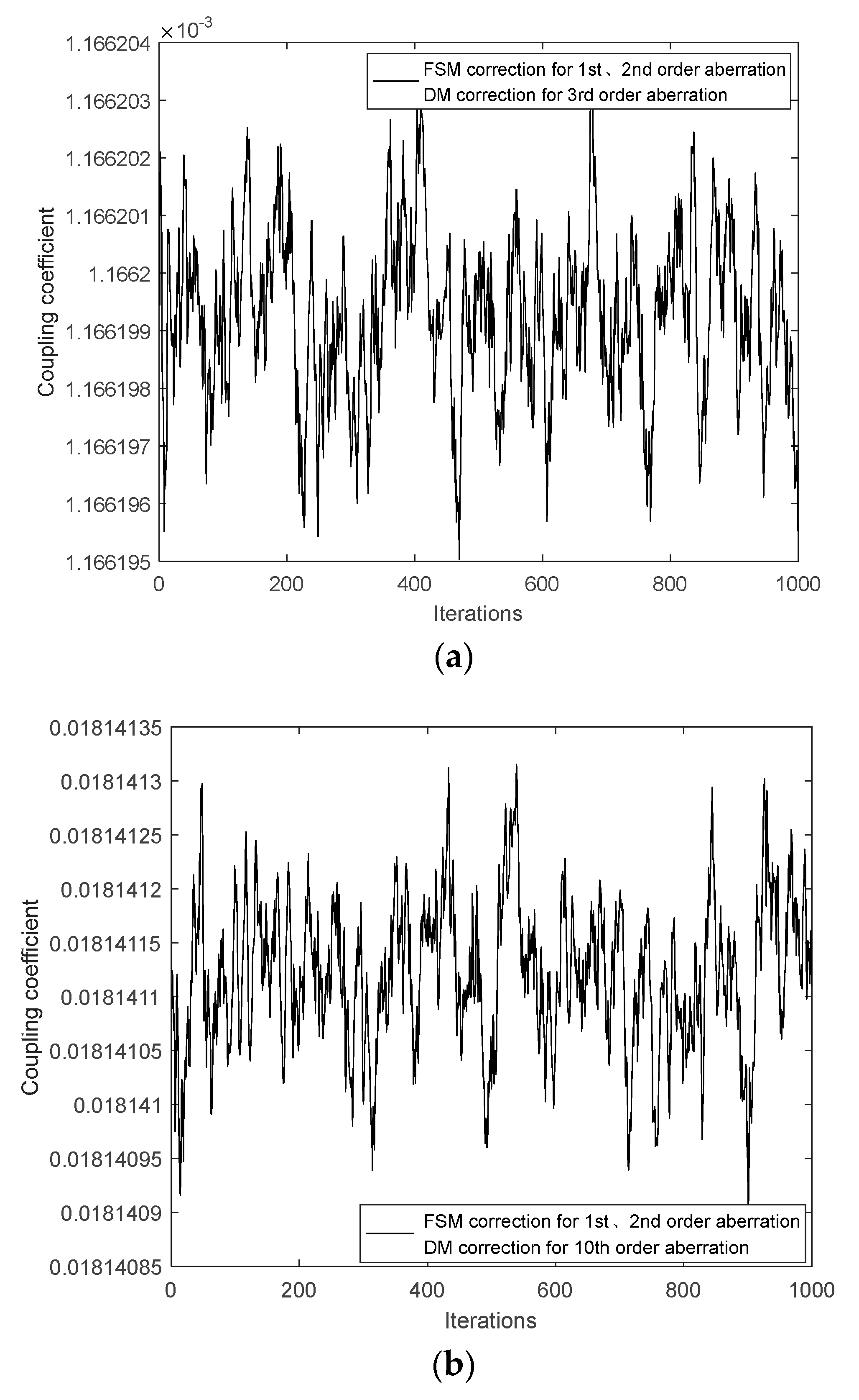
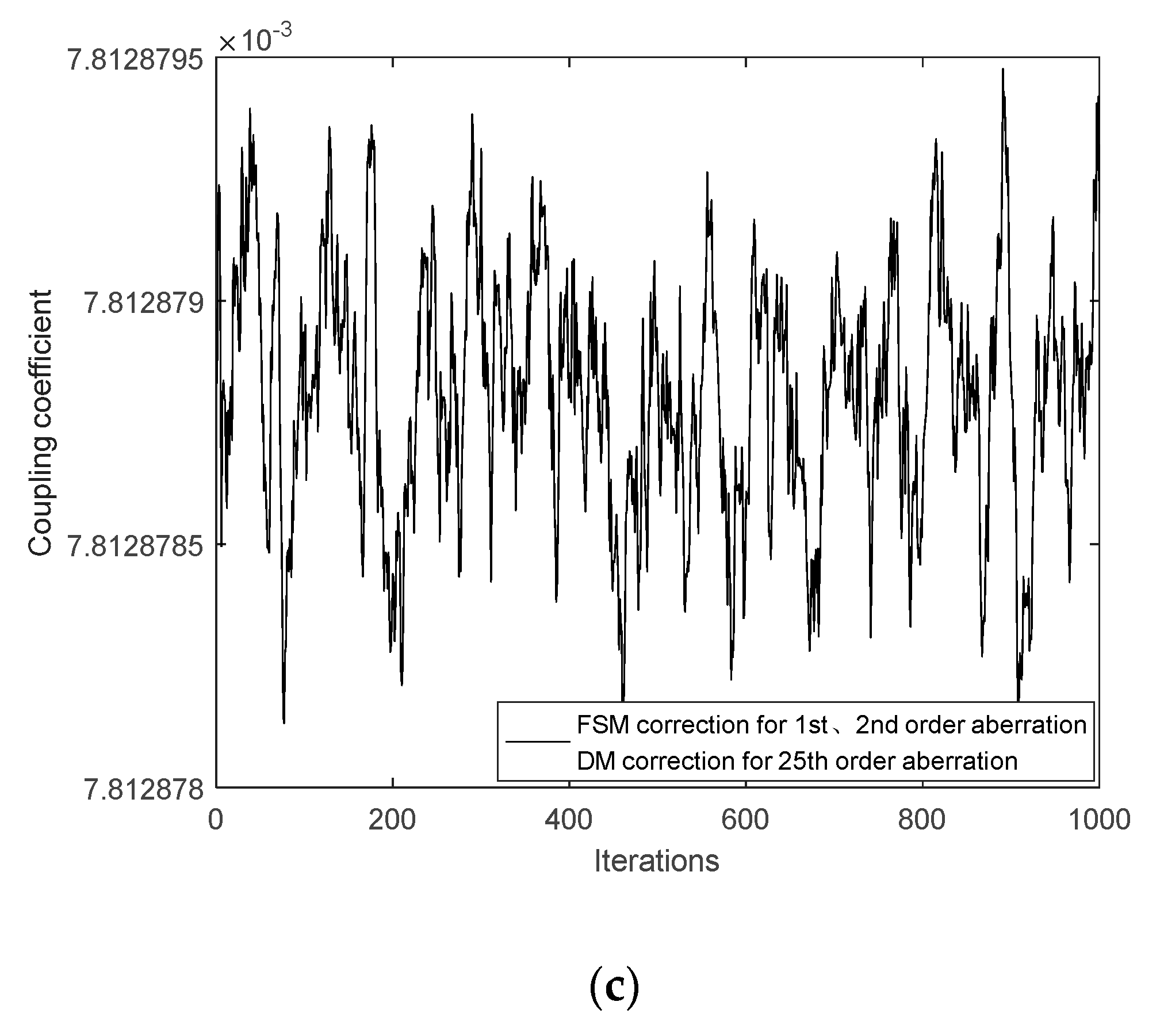
5. Coupling Analysis

The coupling coefficient is calculated from the directional cosine of the Woofer phase compensation and the Tweeter phase compensation. This coefficient represents the degree of correlation between them [17]. Through research, the coupling effect of the dual-deformable-mirrors wavefront correction system can be effectively reduced, achieving independent correction of each order of aberrations and correction of any order of aberrations, as well as targeted correction of specific aberrations in different scenes. This will make the dual-deformable-mirrors wavefront correction system more widely used and lay the foundation for the application of large aperture telescopes. For example, when correcting 3rd-order aberrations, the mode coefficients of the aberrations are 0.657761, 2.42713, and 0.0423 μm. Figure 8 shows the saturation margin of the DM actuator and the coupling coefficient curve between the FSM and the DM.
Figure 8a depicts the coupling coefficient curve between the FSM and the DM. Figure 8b displays the saturation margin of the DM actuator. By combining Figure 8a,b, the black line in Figure 8a represents the coupling coefficient curve when correcting the 1st-order and 2nd-order aberrations of the FSM and the 1st-, 2nd- and 3rd-order aberrations of the DM. The red line represents the coupling coefficient curve when correcting the 1st- and 2nd-order aberrations of the FSM and the 3rd-order aberration of the DM. The black line in Figure 8b represents the saturation margin of the DM actuator, corresponding to the black line in Figure 8a. The red line represents the saturation margin of the DM actuator, corresponding to the red line in Figure 8a. As can be seen from the black line in Figure 8b, it is evident that the saturation margin of some actuators of the DM decreases rapidly, which reduces the ability to correct aberrations and affects the correction of more high-order aberrations. This will seriously affect the stroke of the DM actuator, resulting in resource waste and increased costs. Therefore, the decoupling study of the dual deformable mirrors wavefront correction system is crucial.

6. Conclusions

This article presents a decoupling algorithm for a dual-deformable-mirrors wavefront correction system. The algorithm utilizes Zernike coefficients to directly represent the compensating ability of the DM and enables independent correction of each order of aberration. Based on the expression formula of the coupling coefficient in a typical dual-deformable-mirrors wavefront correction system, this study analyzes the coupling effect of correcting different aberrations and draws the following conclusions:
(1)
The utilization of a typical dual-deformable-mirrors wavefront correction system can achieve independent correction of various order aberrations and targeted correction of specific aberrations in different scenes, effectively suppressing the coupling effect between deformable mirrors.
(2)
The algorithm studied in this paper is simple and feasible, and it has been verified that the algorithm can be applied to the feasibility of the dual-deformable-mirrors wavefront correction system with a wavefront sensor. This research holds great practical significance in engineering and provides an important reference basis for its practical applications.

Author Contributions

Conceptualization, X.K.; methodology, J.L. and H.W.; software, H.W.; validation, J.L., H.W., M.H. and X.K.; formal analysis, X.K.; investigation, M.H.; resources, J.L.; data curation, J.L., M.H. and H.W.; writing—original draft preparation, H.W.; writing—review and editing, J.L. and H.W.; supervision, X.K.; project administration, H.W. All authors have read and agreed to the published version of the manuscript.

Funding

The Key Industrial Innovation Chain Project of Shaanxi Province [grant number 2017ZDCXLGY-06-01]; the General Project of National Natural Science Foundation of China [grant number 61377080]; the Xi’an Science and Technology Planning Project [grant number 2020KJRC0083]; and the Xi’an Science and Technology Plan (22GXFW0115).

Institutional Review Board Statement

The study did not require ethical approval.

Informed Consent Statement

The study did not require ethical approval.

Data Availability Statement

The data or code cannot be made publicly available. Data sharing is not applicable to this article because of the limitations of our patent work.

Conflicts of Interest

The authors declare no conflict of interest.

Nomenclatures

The following nomenclatures are used in this manuscript:
FSMFast-steering mirror
DMDeformable mirror
WooferFSM or a large stroke, low spatial-frequency DM
Tweetera 69-unit DM or a small stroke, high spatial-frequency DM
PVPeak-to-Valley
RMSRoot-Mean-Square
NOPNumerical Orthogonal Polynomials
PIProportional Integral

References

  1. Gerard, B.L.; Dillon, D.; Cetre, S.; Jensen-Clem, R. First laboratory demonstration of real-time multi-wavefront sensor single conjugate adaptive optics. SPIE 2023, 12680, 570–576. [Google Scholar]
  2. Liu, W.; Dong, L.; Yang, P.; Xu, B. Zonal decoupling algorithm for dual deformable mirror adaptive optics system. Chin. Opt. Lett. 2016, 14, 020101–020105. [Google Scholar]
  3. Sivokon, V.P.; Vorontsov, M.A. High-resolution adaptive phase distortion suppression based solely on intensity information. J. Opt. Soc. Am. A 1998, 15, 234–247. [Google Scholar] [CrossRef]
  4. Liu, W.; Dong, L.; Yang, P.; Lei, X.; Yan, H.; Xu, B. A Zernike mode decomposition decoupling control algorithm for dual deformable mirrors adaptive optics system. Opt. Express 2013, 21, 23885–23895. [Google Scholar] [CrossRef] [PubMed]
  5. Zhao, W.; Zhao, M.; Wang, S.; Yang, P. Influence of near ground phase vortex on correction of adaptive optics. Chin. J. Quantum Electron. 2020, 37, 466–476. [Google Scholar]
  6. Cheng, T.; Liu, W.; Pang, B.; Yang, P.; Xu, B. A slope-based decoupling algorithm to simultaneously control dual deformable mirrors in a woofer–tweeter adaptive optics system. Chin. Phys. B 2018, 27, 1–9. [Google Scholar] [CrossRef]
  7. Kong, L.; Cheng, T.; Yang, P.; Wang, S.; Yang, C.; Zhao, M. Decoupling control algorithm based on numerical orthogonal polynomials for a woofer-tweeter adaptive optics system. Opt. Express 2021, 29, 22331–22344. [Google Scholar] [CrossRef] [PubMed]
  8. Yang, S.; Ke, X. Experimental study on adaptive optical wavefront correction with dual mirrors in free space optical communication. Optik 2021, 242, 1–12. [Google Scholar] [CrossRef]
  9. Liu, W.; Xv, B.; Sun, W. Decoupling Control Algorithm Used for Wave Front Sensor-Free Adaptive Optics System with Dual Deformable Mirrors Based on Mode Project-Constraint. Chin. J. Lasers 2023, 50, 106–112. [Google Scholar]
  10. Zou, W.; Qi, X.; Burns, S.A. Woofer-tweeter adaptive optics scanning laser ophthalmoscopic imaging based on Lagrange-multiplier damped least-squares algorithm. Biomed. Opt. Express 2011, 2, 1986–2004. [Google Scholar] [CrossRef] [PubMed]
  11. Hu, M. A Review of Simulation Methods for the Optical Wavefront Distorted by Atmospheric Turbulence. Opt. Optoelectron. Technol. 2003, 1, 10–12. [Google Scholar]
  12. Yang, W.; Wang, J.; Wang, B. A method used to improve the dynamic range of Shack–Hartmann wavefront sensor in presence of large aberration. Sensors 2022, 22, 7120–7134. [Google Scholar] [CrossRef] [PubMed]
  13. Noll, R.J. Zernike polynomials and atmospheric turbulence. J. Opt. Soc. Am. 1976, 66, 207–211. [Google Scholar] [CrossRef]
  14. Hu, Z.; Jiang, W. Simulation of the Optical Wavefront Distorted by Atmospheric Turbulence. Opto-Electron. Eng. 1995, 22, 50–56. [Google Scholar]
  15. Xv, C.; Hao, S.; Wang, Y.; Zhao, Q.; Liu, Y. Atmospheric Turbulence Distortion Wave-Front Reconstruction Based on Modal Mutual Information. J. Air Force Eng. Univ. 2020, 21, 65–70. [Google Scholar]
  16. Wu, Y. Application Research of Adaptive Optics Technique in Atmospheric Optical Communications; Graduate School of Chinese Academy of Sciences (Institute of Optoelectronics Technology): Beijing, China, 2013. [Google Scholar]
  17. Wu, J. The Beauty of Mathematics in Computer Science; Posts and Telecommunications Press: Beijing, China, 2012. [Google Scholar]
Figure 1. Schematic diagram of dual-deformable-mirrors wavefront correction system.
Applsci 13 12112 g001
Figure 2. Flowchart of separation coefficient algorithm.
Applsci 13 12112 g002
Figure 3. Initial wavefront distortion. (a) Zernike coefficient. (b) Wavefront distortion phase diagram.
Applsci 13 12112 g003
Figure 4. Wavefront phase diagrams. (a) Wavefront phase diagram after FSM correction. (b) Wavefront phase diagram after DM correction. (c) Wavefront phase diagram after both FSM and DM correction.
Applsci 13 12112 g004
Figure 5. Coupling coefficient curve between the FSM and the DM.
Applsci 13 12112 g005
Figure 6. Experimental diagram of typical adaptive optics dual-deformable-mirrors wavefront correction system.
Applsci 13 12112 g006
Figure 7. Coupling coefficient curve between FSM and DM.(a) FSM only corrects the 1st and 2nd-order aberrations, DM only corrects the 3rd-order aberrations (b) FSM only corrects the 1st and 2nd-order aberrations, DM only corrects the 10th order aberrations (c) FSM only corrects the 1st- and 2nd-order aberrations, DM only corrects the 25th-order aberrations.
Applsci 13 12112 g007aApplsci 13 12112 g007b
Figure 8. Curves. (a) Coupling coefficient curve. (b) Saturation margins of DM actuators.
Applsci 13 12112 g008
Table 1. Aberration expressions for the first 15 orders Zernike polynomials.
i(n, m)Polar CoordinatesCartesian CoordinatesAberration Type
1(0, 0)11Piston
2(1, 1) 2 ρ cos θ 2xX-direction Tilt
3(1, −1) 2 ρ sin θ 2yY-direction Tilt
4(2, 0) 3 2 ρ 2 1 3 2 x 2 + 2 y 2 1 Defocus
5(2, −2) 6 ρ 2 sin 2 θ 2 6 x y Y-direction Coma
6(2, 2) 6 ρ 2 cos 2 θ y 2 x 2 X-direction Coma
7(3, −1) 2 2 3 ρ 3 2 ρ sin 2 θ 2 2 3 x 3 + 3 x y 2 2 x Y-direction Astigmatism
8(3, 1) 2 2 3 ρ 3 2 ρ cos 2 θ 2 2 3 x 3 + 3 x y 2 2 y X-direction Astigmatism
9(3, −3) 2 2 ρ 3 sin 3 θ 2 2 3 x y 2 x 3 Trefoil Aberration
10(3, 3) 2 2 ρ 3 cos 3 θ 2 2 y 3 3 x 2 y Trefoil Aberration
11(4, 0) 5 6 ρ 4 6 ρ 2 + 1 5 6 y 4 + 12 x 2 y 2 + 6 x 4 6 x 2 6 y 2 + 1 Spherical Aberration
12(4, 2) 10 4 ρ 4 3 ρ 2 cos 2 θ 10 4 y 4 4 x 4 + 3 x 2 3 y 2
13(4, −2) 10 4 ρ 4 3 ρ 2 sin 2 θ 10 8 x y 3 + 8 x 3 y 6 x y
14(4, 4) 10 ρ 4 cos 4 θ 10 x 4 6 x 2 y 2 + y 4 Quatrefoil Aberration
15(4, −4) 10 ρ 4 sin 4 θ 10 4 x y 3 4 x 3 y Quatrefoil Aberration
Disclaimer/Publisher’s Note: The statements, opinions and data contained in all publications are solely those of the individual author(s) and contributor(s) and not of MDPI and/or the editor(s). MDPI and/or the editor(s) disclaim responsibility for any injury to people or property resulting from any ideas, methods, instructions or products referred to in the content.

