Brake Squeal Investigations Based on Acoustic Measurements Performed on the FIVE@ECL Experimental Test Bench

Abstract

Radiated noise is a major topic of interest regarding the brake squeal phenomenon as it is directly linked to the noise generated which can be potentially detrimental to user comfort and perception. However, very few studies offer in-depth and comprehensive insight into the analysis and understanding of acoustic noise during squeal events. This study is intended to provide an original contribution to this issue by investigating acoustic phenomena occurring during the squeal phenomenon via a digital antenna composed of 117 microphones. Experiments are performed on the Friction-Induced Vibration and noisE test bench at Ecole Centrale de Lyon (FIVE@ECL). The first main aim is to investigate the characteristics of the acoustic radiated field during brake squeal and more particularly to describe the evolution of the radiated field patterns per revolution of the disc system. The second major aim is to illustrate the possibility of reconstructing the radiated acoustic field everywhere in the space surrounding the brake system, leading to the construction of a robust representation of 3D acoustic patterns, providing acoustic squeal events in the physical space around the brake system. Results show that the vibratory signature remains identical during squeal event braking test. The acoustic signature of squeal noise consists mainly of a fundamental frequency and its harmonic components, with secondary lower contributions from other fundamental frequencies. The associated radiated acoustic field during squeal events are characterized by different directivities and intensities of the acoustic radiated field for each squeal frequency, with potential changes in these directivities and intensities over short times corresponding to the rotation period of the disc.

1. Introduction

The problem of friction-induced self-excited vibrations and acoustic radiation has been widely studied for many years as it is one of the major problems encountered in the design of industrial brake systems. General reviews on this subject can be found in [1,2,3,4,5]. Despite the large number of studies that have been carried out on this subject, understanding the physical phenomena involved in brake squeal and predicting squeal noise remain a major concern in many industrial applications related to the automotive [6,7,8,9,10,11], aeronautical [12,13] and railway [14,15,16,17] sectors. Indeed, the study of brake squeal is a multi-physics problem that requires advanced analysis in various fields such as vibration, tribology, thermodynamics and acoustics, for example. As a result, academic test rigs [18,19,20,21,22,23,24,25,26,27] have been developed in order to propose experimental contributions in order to better understand friction-induced vibrations and noise.

Although many experimental studies have been carried out to investigate the problems of friction-induced vibration, only a few experimental studies have so far been conducted to investigate the impact of squeal noise on the basis of the resulting radiated sound field. In most cases, a single microphone is used to measure squeal noise, which does not allow the complete and consistent analysis of radiated noise during squeal events. Although a study of the link between friction-induced vibrations and squeal noise using acoustic measurements with a nine-microphone antenna was recently carried out by authors of [26]; these previously proposed results do not allow detailed analysis of the radiated field. Furthermore, specific studies on the acoustic holography of brake squeal have also been performed to measure the movement of the disc and the associated travelling waves [28,29]. Thus, Flint and Hald [29] used acoustic measurements to estimate the parietal velocity field of a braking system to characterise its dynamic behaviour. The near-field acoustic measurements were processed, and an inversion algorithm was used to reconstruct the parietal estimates. This study highlighted wave propagation phenomena, showing the appearance of travelling waves, whose direction of progression changes during squeal. More generally, the problems of source identification can be addressed by performing near-field pressure measurements [29,30]. However, the direct acoustic field in the surrounding space has never been studied in detail, i.e., in terms of temporal evolution, sound level, as well as directivity characterization. This question is one of the contributions of the present study, the main objective of which is to characterise the squeal phenomenon from the point of view of acoustic radiation by deploying pressure measurement devices in front of the braking system subjected to vibrations induced by friction and acoustic noise. With regard to this objective, although the braking system and operating conditions considered are similar to those already proposed in previous studies [25,26], here, we focus more specifically on the analysis of the radiated sound field and the characterization of the squeal frequencies in terms of amplitude and acoustic directivity, by carrying out pressure measurements for a large number of test points. In order to achieve this goal, a 1.5 m diameter antenna with 117 microphones is used to determine the acoustic field and describe it over a large surface and not just at a limited number of spatial points. Thus, it is possible to carry out an analysis of the acoustic radiated field and obtain the characterization of squeal noise by the direct exploitation of these pressure measurements. To the best of our knowledge, this type of acoustic characterization for the problem of friction-induced vibration and noise for brake systems has not yet been addressed in the literature.

Furthermore, a second objective is to apply a well-known method (i.e., the SONAH method described in [31]) to reconstruct the radiated acoustic field so as to visualize, for a given test and a series of pressure measurements carried out, the radiated acoustic field everywhere in the surrounding space of the brake system. With regard to the second objective, the aim is to use the measurements to apply a method to rebuild the acoustic field not only at the measurement points but globally, thereby permitting the complete visualization of the acoustic field in space. We recall that it is not possible to vary the position of the microphones in a specific braking test or compile different braking tests with different microphone positions, as the problem of vibration and friction-induced noise is characterized by a potentially complex non-linear behaviour that evolves over time. Moreover, while having a greater number of microphones makes it possible to have more complete information on the pressure field on one surface, it is not sufficient to systematically ensure the detailed visualization of acoustic phenomena, which can vary greatly over a small distance. Therefore, we propose to implement a pressure field reconstruction method that is frequently used, notably in the framework of acoustic source detection problems [31,32,33].

This paper is organized as follows. First of all, a brief reminder of the general description of the laboratory brake system known as Friction-Induced Vibration and noisE at the Ecole Centrale de Lyon (FIVE@ECL) and the experimental device used for the study are discussed. Then, the pressure measurements are analyzed to characterize the different frequencies involved in squeal noise. In the following sections, a method for reconstructing the acoustic field is discussed and validated on the basis of experimental tests performed on the brake system under study. Furthermore, we demonstrate the feasibility of globally reconstituting the radiated acoustic field in the whole 3D space in the vicinity of the brake system, thus providing a substantial and original improvements to the description of radiated noise during squeal events.

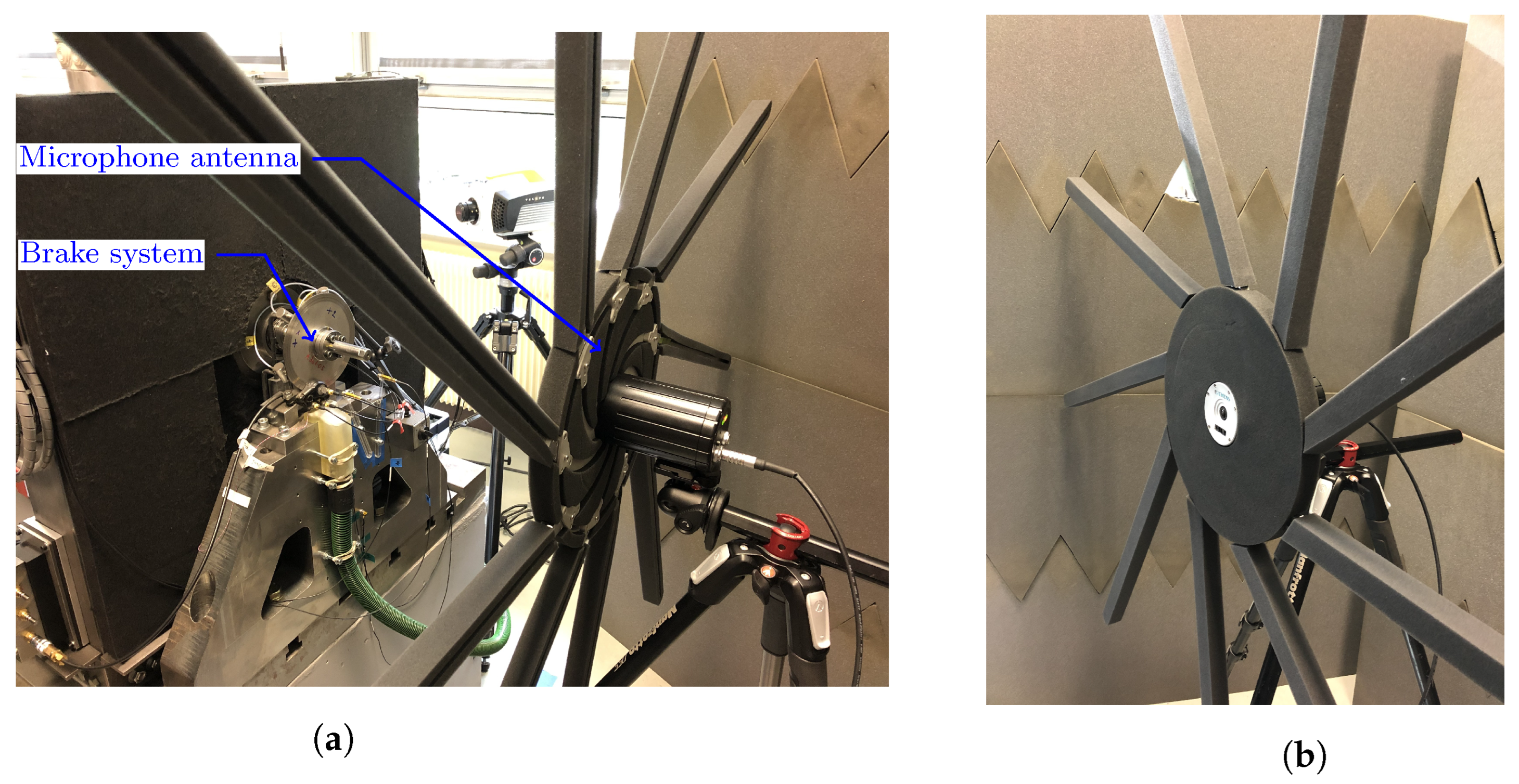
2. Description of the Experimental FIVE@ECL Test Bench and Data Acquisition

A detailed description as well as the main characteristics of the experimental FIVE@ECL test bench can be found in [25]. More specifically with respect to the brake system under study, it is composed of one disc with a 0.16 m external diameter, 0.033 m internal diameter and a thickness of 0.002 m, two F03C pads and a caliper XT M785 from the Japanese manufacturer Shimano. Figure 1a shows the braking system for the experimental FIVE@ECL test bench.

In order to analyze and characterize the squeal phenomenon and the associated radiated noise, braking tests are conducted through the programmed variation of the pressure to the pads and speed to the disc rotation. These two parameters correspond to the two operational parameters monitored during a braking test whereas the motor torque and the temperature are non-controlled and measurable operational parameters directly resulting from the braking test conditions. The choice is made to perform a constant speed braking test, a protocol classically used in the field of friction-induced vibration and noise on academic test benches. The main objective is to limit the number of operating parameters (such as rotation speed) and to illustrate the fact that brake squeal occurs not only when the rotation speed of the disc is slowing down, which has already been discussed in [17,25].

Figure 2 illustrates the experimental protocol with the different phases and the time evolution of the four operational parameters (i.e., the rotating speed of the disc, the motor torque, the brake pressure and the pad temperature) during a braking test. The protocol for one braking test is defined as follows:

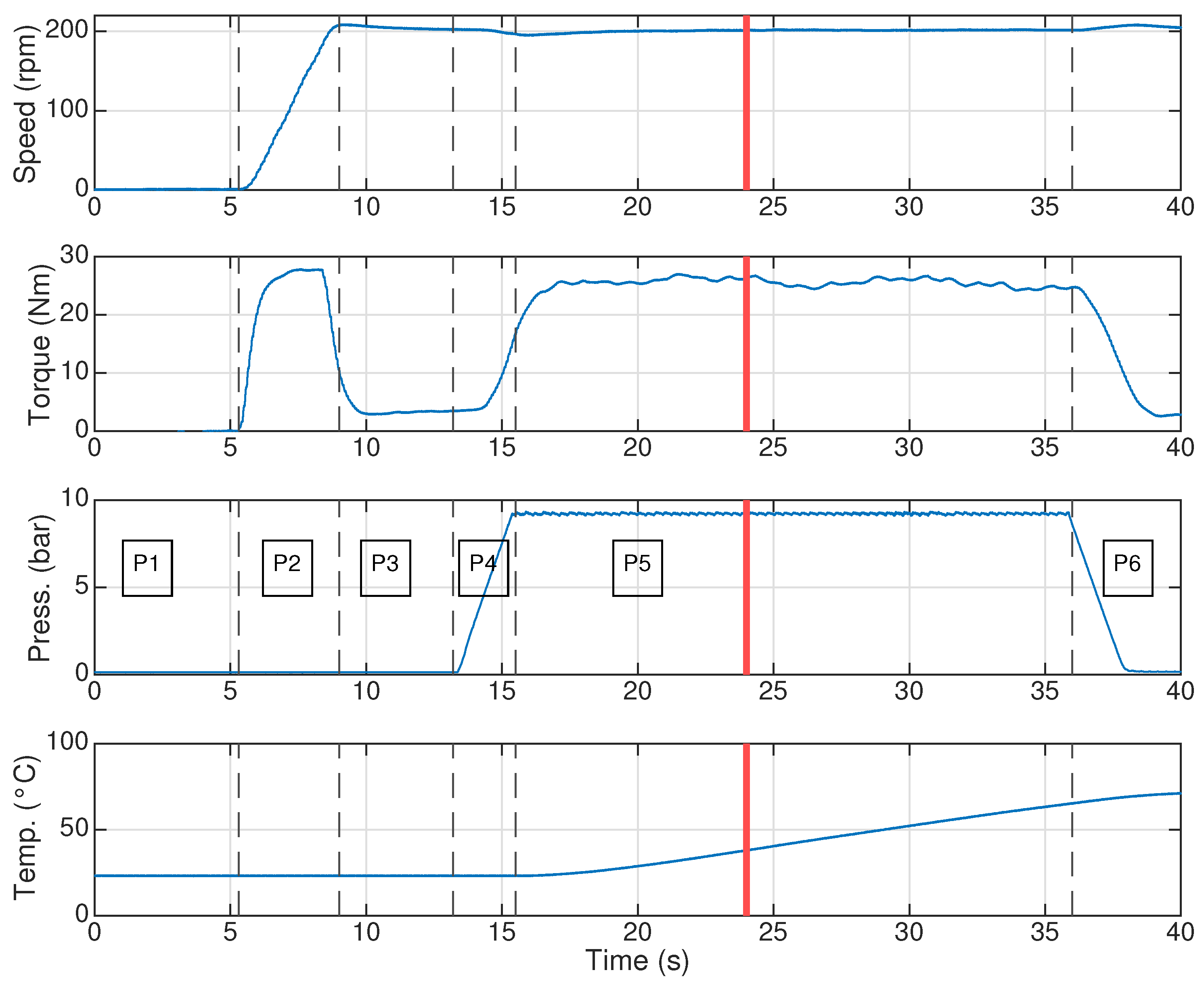
• $t=0$ s: braking system at rest and the start of data acquisition;
• 0 s $<t<$ 5.3 s: Phase 1—no rotation;
• 5.3 s $<t<$ 9 s: Phase 2—increasing the rotation of the disc from 0 to 200 rpm (keeping the brake pressure at zero);
• 9 s $<t<13.2$ s: Phase 3—system rotating at 200 rpm without brake pressure;
• 13.2 s $<t<$ 15.5 s: Phase 4—rise in brake pressure from 0 to 9 bars. This period corresponds to the pads and the disc coming into contact along with the emergence of friction-induced vibrations and squeal noise;
• 15.5 s $<t<$ 36 s: Phase 5—braking phase by keeping the brake pressure at nine bars and the disc rotation speed at 200 rpm;
• $t>$ 36 s: Phase 6—brake pressure release.

The different phases of the protocol are indicated on the Figure 2 by the notation Pi for the ith phase (with i $=1,\dots ,6$). In the rest of the study, we focus on the analysis of the radiated noise in the time interval $t\in [16;35]$ s, which is the phase of the braking test where the squeal phenomenon is established and the brake pressure and rotation of the disc are constant.

As previously explained, one of the main originalities of the present work is to provide a detailed and in-depth analysis of the radiated noise during a braking test to characterize squeal noise. In order to achieve this objective, it is necessary to set up a specific experimental system to accurately measure the radiated field over a large number of test points. The measurements are carried out in collaboration with the company MicrodB by using an LMS SoundCam 1.5 m large digital antenna with 117 microphones, as shown in Figure 1b. The position of each microphone in the plane of the antenna is shown in Figure 3. This digital microphone antenna is modular enough to cover a wide frequency range (from 100 to 20,000 Hz). The position of the digital microphone antenna in relation to the braking system is chosen at 0.12 m. More precisely, it corresponds to the distance between the microphone array plane and the disc plane, i.e., the distance between the center of the antenna (aligned with the the center of the brake disc) and the brake disc system. It should be noted that the distance between the center of the disc and each microphone is slightly different, which is taken into account for the acoustic field reconstruction discussed in Section 4. In addition, in order to better reproduce free field conditions and ensure the predominance of the direct field, absorbing panels are placed around the antenna, as illustrated in Figure 1b.

3. Experimental Study of Squeal Noise

The first objective of this study is to characterize the squeal noise by analyzing the acoustic signature during a braking test. Firstly, a preliminary analysis based on the estimation of the decay of the sound pressure as a function of distance between a microphone and the center of the brake disc and the frequency content of squeal noise during a braking test are investigated. Secondly, the characteristics of each frequency based on squeal noise identified are analyzed in greater detail.

3.1. Preliminary Analysis

The preliminary analysis of the tests carried out is conducted in two steps.

Firstly, the evolution of the mean square pressure as a function of distance for each microphone from the braking system (which corresponds to the origin of squeal noise) is estimated by analyzing the experimental results of the temporal evolution of the squeal noise. For each microphone, the mean square of the temporal signal is estimated for 15.5 s $<t<$ 36 s (i.e., on the phase of the braking test when the squeal noise is generated). Figure 4 shows a cloud of points obtained from the measurements carried out in one braking test. A decrease in the signal almost proportional to the square of the distance is observed (i.e., the decrease is more precisely identified as equal to $\frac{1}{r^{1.94}}$). This result allows us a regorous conduct of our study, knowing that the experimental results are not related to external disturbances (such as unwanted reflections due to non-controlled experimental conditions, for example).

Secondly, Figure 5 illustrates the spectrogram obtained from one typical evolution of squeal noise by considering one microphone of the digital antenna. A Fourier transform is calculated with a time window $\Delta t=\frac{0.1}{3}$ s, the sampling frequency of the measurements being 56,250 Hz. It can be observed without any ambiguity that the squeal noise generated for $t>15.5$ s is mainly composed of one fundamental frequency $f_1=610$ Hz and the associated harmonic components denoted by $f_2=2f_1=1220$ Hz, $f_3=3f_1=1830$ Hz, $f_4=4f_1=2440$ Hz and $f_5=5f_1=3050$ Hz. These results are of course in agreement with those of previous studies [25,26]. Moreover, some additional phenomena due to thermal effects can also be the cause of complex secondary transient phenomena during squeal events. This is characterized by several additional second-order contributions corresponding to frequencies that decrease during squeal events (as observed in the frequency ranges $[900;1200]$ Hz and $[1200;1600]$ Hz). For more details on these unexpected thermal effects on squeal events, the reader can refer to [27].

For the rest of the study, we focus on frequencies $f_1$, $f_2$, $f_3$, $f_4$ and $f_5$ that correspond to the main contributions of squeal noise. Moreover, to illustrate the effectiveness of the methodology to reconstruct the acoustic field from measurements in the near field, the results presented in the following sections are proposed only at $t=24$ s (denoted by the red lines in Figure 2 or the dashed line in Figure 5) for which the five frequencies of interest are clearly visible. The acoustic phenomenon of squeal over the entire duration of the braking test remains outside the scope of this study and will be the subject of future work. Nevertheless, we check that the acoustic behavior remains relatively the same for several seconds. Hence, the results proposed here are not specific for one specific time interval (i.e., $t=24$ s) but remain valid during squeal events.

It should be noted that the potential links between the emergence of friction-induced vibrations and squeal noise in the near-field and far-field were discussed in depth previously in [26]. Although the frequency signature observed in vibration is similar to that analyzed on radiated noise during transient and stationary squeal events, it is observed that the largest frequency contributions of squeal noise are not necessarily the largest frequency contributions of the friction-induced vibrations detected on the two pads, the disc and the caliper. It can therefore be concluded that there is no obvious link between the acoustic levels and the vibration levels for each frequency contribution. In addition, for a more detailed comment on the phenomena of friction-induced vibrations during squeal events, the interested readers should refer to [25]. It is noteworthy that the repeatability validation of squeal events observed on the FIVE@ECL test bench was discussed in previous studies [25]. In conclusion, the previous results published in [26] also demonstrate the interest of performing a specific analysis of squeal noise for a more detailed investigation of the squeal phenomenon, as proposed in the context of the present study.

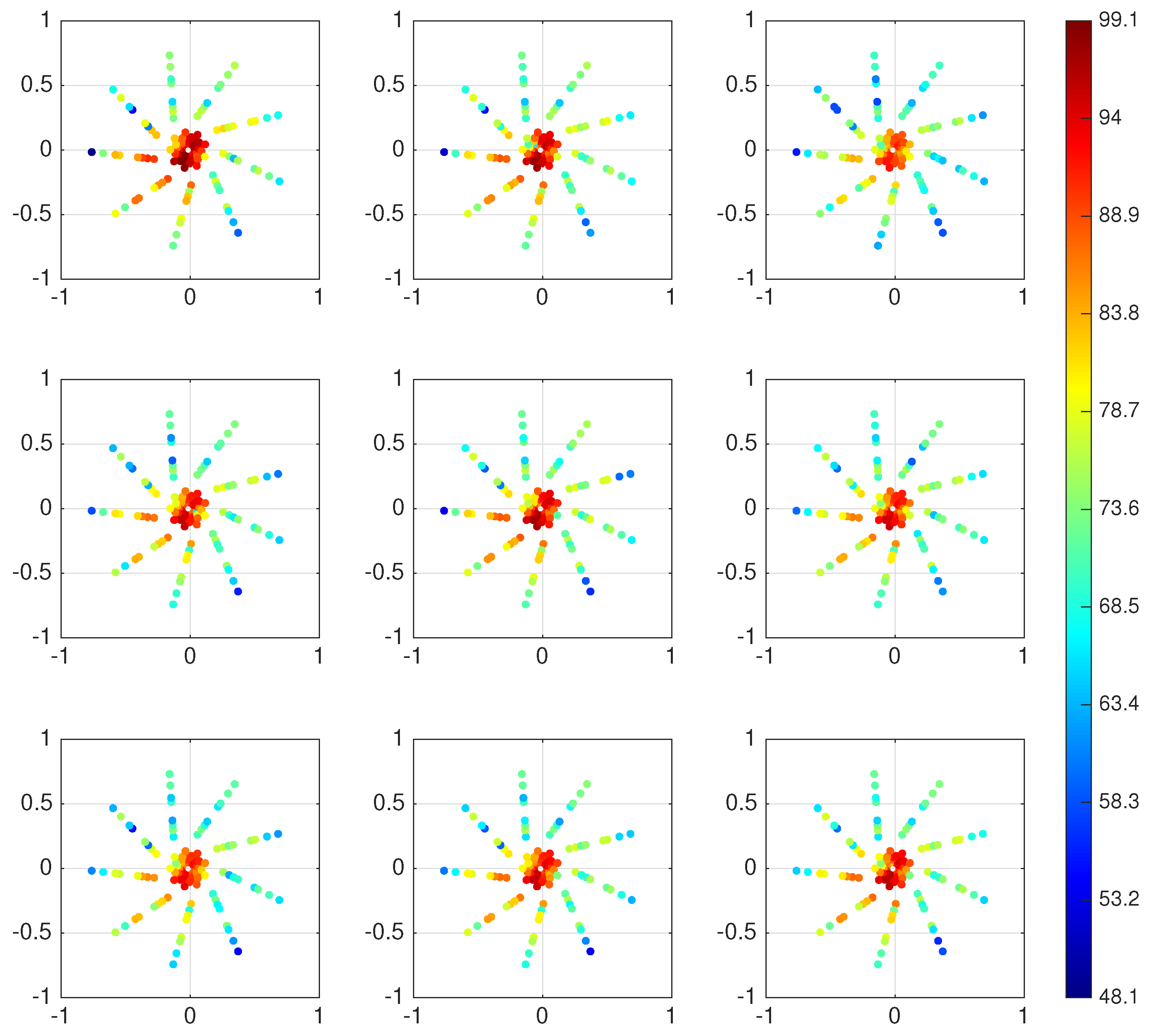
3.2. Characterisation of Squeal Frequencies

In this section, we are interested in a more precise characterization of the acoustic radiation associated with frequencies $f_1$, $f_2$, $f_3$, $f_4$ and $f_5$ previously identified in Figure 5. The objective is to provide an understanding of squeal noise and its transient evolution over short times associated with the rotation period of the brake system. Due to the fact that the rotation speed of the disc is 200 rpm, the transient evolution over time of each frequency component of the squeal noise is analyzed over two revolutions using nine pictures per revolution, starting at $t=24$ s. It is verified that this choice of discretization in time is sufficient to properly capture the temporal evolution of the acoustic diagram over a period of rotation, not only in terms of level but also in terms of directivity. In order to conduct this study, a Fourier transform is calculated with a time window $\Delta t=0.03$ s, which represents a compromise making it possible to isolate and define the local spatial behavior of the acoustic radiation while keeping a good approximation of the frequency estimate, as the sampling frequency of the measurements is 56,250 Hz.

Figure 6, Figure 7, Figure 8, Figure 9 and Figure 10 illustrate the evolution of the squeal noise for all the microphones of the digital antenna and at each frequency of interest (i.e., $f_1$, $f_2$, $f_3$, $f_4$ and $f_5$). The temporal evolution of the acoustic radiation must be viewed from left to right, in sequence from top to bottom. The pictures are displayed evenly over time by considering two periods of disc revolution. In other words, nine views of the acoustic pattern are taken per time interval corresponding to one revolution of the disc, these views being taken with identical time intervals between each of them (i.e., $\Delta t=0.33$ s).

At $f_1$ and $f_2$, a variation in terms of both level and directivity that can be linked to the rotating speed of the disc can be observed, although this phenomenon is less pronounced for $f_2$. The maximum level for $f_2$ is lower than that for $f_1$. When comparing the results during the first and the second revolutions (see the nine first pictures compared with the nine last pictures in Figure 6), the temporal evolution of both the pattern and the level are similar. This illustrates good repeatability of the characteristics of the squeal noise decomposed over these frequencies with a repeatable evolution over a period of revolution of the disc. It can also be noted that the maximum level for $f_2$ remains localized at half $x>0$ (see Figure 3), although the directivity is not constant on one revolution of the disc. At $f_3$, the acoustic radiation has a relatively homogeneous directivity and level on the two revolutions of the disc. The maximum level is close to that observed for the first frequency $f_1$ and the directivity is characterized by a level maximum which remains at half $x<0$. The squeal noise related to $f_4$ is characterized by a high level around 100 dB. Contrary to the results previously discussed for the first three frequencies, the evolution of the acoustic radiation per revolution is relatively stable for $f_4$ and the directivity reveals a high level located in the centre of the microphone antenna and mainly oriented along a diagonal at 45 degrees to the x-axis. Finally, the highest acoustic level is obtained for $f_5$. Although the acoustic level seems fairly homogeneous and located at the center of the antenna over the two revolutions of the disc, the directivity seems to be linked to the periodicity of a revolution of the disc and mainly oriented along a diagonal at 45 degrees to the x-axis. In conclusion, this analysis illustrates that evolutions per revolution of the radiated acoustic fields for the contribution of the five main frequencies during a braking test can be complex and very different for each frequency. They are further characterized by three main criteria (cf.

Table 1. Criteria used to characterize the five first frequencies.

	${\mathit{f}}_1$	${\mathit{f}}_2$	${\mathit{f}}_3$	${\mathit{f}}_4$	${\mathit{f}}_5$
Max sound level	91.2 dB	80.4 dB	90.6 dB	99.1 dB	101.4 dB
Shape variation per disc revolution	yes	yes	no	no	no
Directivity	cf. figures and description in the body of the text.

): the maximum sound level and its localization, the directivity of the acoustic radiation and the periodic or non-periodic evolution of the acoustic pattern and level per revolution of the disc.

It is worth noting that in the proposed study, the analysis is carried out by examining the directivity of the squeal noise and its evolution over time relative to the fixed brake reference frame. There are two reasons for this choice: the first one is that some elements of the disc (caliper, pads) do not rotate and the friction zone that generates the brake squeal and the associated radiated noise is therefore immobile in the fixed frame of reference. The second reason relates to the experimental set-up itself, since the system for measuring radiated noise is non-rotating. Instead of examining the time variation of squeal noise in the fixed brake reference frame it would also be possible to interpret the time variation that the pictures show as a sound emitted at the frequency of the brake rotation. However, in the latter case, it would not be possible to easily dissociate the acoustic filed emitted which are non-rotating and rotating over time in the fixed frame of the brake system, knowing that such results then make it possible to offer first analyses on the fact that the squeal noise comes from fixed parts, rotating parts or a combination of both.

4. Acoustic Field Reconstruction

The first part of this study focused on providing basic understanding of the evolution of the radiated acoustic fields per disc revolution and conclusions on the characterization of squeal noise on the main frequencies of interest. In the following, a methodology is presented for reconstructing acoustic quantities based on acoustic pressure measurements obtained from the digital microphone antenna situated at 0.12 m in front of the braking system.

This section is organized as follows: first, the method for reconstructing 3D acoustic quantities based on acoustic pressure measurements is briefly described. It should be noted that the proposed strategy is based on well-known developments previously published in [31,34,35,36]. The following section of the paper therefore only aims to offer the basic elements for the interested reader who can refer to [31,34,35,36] for more detailed additional explanations. Then, its effectiveness is tested by estimating the radiated acoustic field at the measurement points defined by the 117 microphones of the digital antenna. Finally, the acoustic field is calculated downstream of the acoustic antenna and according to the three spatial dimensions.

4.1. Methods for 3D Reconstruction

The method used for reconstructing acoustic quantities based on acoustic pressure measurements is based on the well-known near-field acoustical holography (NAH) and the statistically optimized NAH (SONAH) method [31,34,35,36]. This method is based on the first step of reconstructing the acoustic field in the free field from acoustic measurements taken in the near field. The reconstruction performed can then be used to define the inverse problem which leads to the localization of the source. In the context of the present study, this methodology is developed to provide a 3D reconstruction of the radiated acoustic field due to squeal noise.

The method consists in reconstructing an acoustic field in a $\Omega$ domain made up of a homogeneous light fluid from pressure measurements. The main assumption is that the reconstructed field can be reconstructed from a series of elementary plane waves noted ${\mathrm{\Psi }}_n$ with $n=1,\cdots ,N$ such that

$$p_i\left({\mathbf{r}}_i\right)=\sum _{n=1}^N{a}_n{\mathrm{\Psi }}_n\left({\mathbf{r}}_i\right),$$

(1)

where $p_i\left({\mathbf{r}}_i\right)$ corresponds to the measured pressures. We note that $i=1,\cdots ,I$, I is the number of available and reliable measurements. Coefficients $a_n$ are the unknowns of the identification problem. This problem can be over-determined or under-determined depending on whether the number of measurements is higher or lower than the number N of coefficients that have to be identified. In order to better represent all the possibilities of acoustic radiation, it is nevertheless advisable to opt for a high value of N. Equation (1) can be written in matrix form such that

$$\mathbf{p}=\mathbf{Ba},$$

(2)

where $\mathbf{p}$ is the vector of pressures $\left\{p_i\left({\mathbf{r}}_i\right)\right\}$, $\mathbf{a}$ is the vector of coefficients $\left\{a_n\right\}$, and $\mathbf{B}$ a matrix containing the values at points ${\mathbf{r}}_i$ of functions ${\mathrm{\Psi }}_n$:

$$\mathbf{B}=\left[\begin{array}{cccc}{\mathrm{\Psi }}_1\left({\mathbf{r}}_1\right)& {\mathrm{\Psi }}_2\left({\mathbf{r}}_1\right)& \cdots & {\mathrm{\Psi }}_N\left({\mathbf{r}}_1\right)\\ {\mathrm{\Psi }}_1\left({\mathbf{r}}_2\right)& {\mathrm{\Psi }}_2\left({\mathbf{r}}_2\right)& & {\mathrm{\Psi }}_N\left({\mathbf{r}}_2\right)\\ ⋮& & \ddots & ⋮\\ {\mathrm{\Psi }}_1\left({\mathbf{r}}_I\right)& {\mathrm{\Psi }}_2\left({\mathbf{r}}_I\right)& \cdots & {\mathrm{\Psi }}_N\left({\mathbf{r}}_I\right)\end{array}\right].$$

(3)

The problem defined by Equation (2) has to be reversed. To achieve this, the following equation is used:

$$\tilde{\mathbf{a}}={\mathbf{B}}^H{\left({\mathbf{BB}}^H+\epsilon \mathbf{I}\right)}^{-1}\mathbf{p},$$

(4)

where symbol ${(.)}^H$ represents the Hermitian transpose and $\epsilon$ the Tikhonov regularization coefficient. We consider $\epsilon ={\left[{\mathbf{A}}^H\mathbf{A}\right]}_{ii}^{-D/10}$ with $D=10$, as recommended by Hald [31] and Gomes [37]. Obtaining $\tilde{\mathbf{a}}$ makes it possible to recalculate the pressure field $\tilde{p}$ everywhere in $\Omega$:

$$\tilde{p}\left(\mathbf{r}\right)=\sum _{n=1}^N{\tilde{a}}_n{\mathrm{\Psi }}_n\left(\mathbf{r}\right).$$

(5)

This equation can also be rewritten in matrix form:

$$\tilde{p}\left(\mathbf{r}\right)={\tilde{\mathbf{a}}}^T\mathit{\alpha }\left(\mathbf{r}\right),\mathit{\alpha }\left(\mathbf{r}\right)=\left\{\begin{array}{c}{\mathrm{\Psi }}_{\mathbf{1}}\left(\mathbf{r}\right)\\ {\mathrm{\Psi }}_{\mathbf{2}}\left(\mathbf{r}\right)\\ ⋮\\ {\mathrm{\Psi }}_{\mathbf{N}}\left(\mathbf{r}\right)\end{array}\right\}.$$

(6)

By combining Equations (4) and (6), the following equation that directly links the calculated pressure in $\mathbf{r}$ and the measured pressures can be obtained such that

$$\tilde{p}\left(\mathbf{r}\right)={\mathbf{p}}^T{\left({\mathbf{A}}^H\mathbf{A}+\epsilon \mathbf{I}\right)}^{-1}{\mathbf{A}}^H\mathit{\alpha }\left(\mathbf{r}\right),$$

(7)

where $\mathbf{A}={\mathbf{B}}^T$.

Then, it is necessary to specify the shapes of functions $\mathrm{\Psi }$. With this in mind, plane wave ${\mathrm{\Phi }}_{\mathbf{k}}$ is defined as follows:

$${\mathrm{\Phi }}_{\mathbf{k}}\left(\mathbf{r}\right)=F\left(k_z\right)e^{-j\left(k_{x}x+k_{y}y+k_z(z-z^{+})\right)},$$

(8)

where F is the amplitude of wave, $z^{+}$ is the plane of the virtual source and $\mathbf{k}=\{k_x,k_y,k_z\}$ is the wave number whose component $k_z$ is defined as follows:

$$k_z=\left\{\begin{array}{cc}\sqrt{k^2-(k_x^2+k_y^2)}\hfill & \mathrm{if}(k_x^2+k_y^2)\le k^2\hfill \\ -j\sqrt{(k_x^2+k_y^2)-k^2}\hfill & \mathrm{if}(k_x^2+k_y^2)>k^2\hfill \end{array}\right.,$$

(9)

with $k^2={\parallel \mathbf{k}\parallel }^2=k_x^2+k_y^2+k_z^2$. The work of Hald [31,38,39] on the SONAH method showed that it is relevant to define the projection functions $\mathrm{\Psi }$ according to the waves defined in Equation (8):

$${\mathrm{\Psi }}_n\left(\mathbf{r}\right)=\kappa {\mathrm{\Phi }}_{k_n}\left(\mathbf{r}\right),\kappa =\sqrt{\frac{\Delta k_x\Delta k_y}{2\pi k^2}}.$$

(10)

$\Delta k_x$ and $\Delta k_y$ result from the discretization of the wave number and therefore from the choice of the number of projection functions used. It is also shown that a good choice of function $F\left(k_z\right)$ is obtained with

$$F\left(k_z\right)=F_0\sqrt{\frac{k}{|k_z|}}.$$

(11)

It is interesting to note that it is possible to calculate matrix ${\mathbf{A}}^H\mathbf{A}$ and vector ${\mathbf{A}}^H\mathit{\alpha }$ to avoid choosing the number of N functions retained. Therefore, as Hald shows for the SONAH method [31],

$${\left[{\mathbf{A}}^H\mathbf{A}\right]}_{ij}=\sum _n{\mathrm{\Phi }}_{k_n}^{*}\left({\mathbf{r}}_i\right){\mathrm{\Phi }}_{k_n}\left({\mathbf{r}}_j\right)\frac{\Delta k_x\Delta k_y}{2\pi k^2}\underset{\begin{array}{c}\Delta k_x\to 0\\ \Delta k_y\to 0\end{array}}{⟶}\frac{1}{2\pi k^2}{\int }_{-\infty }^{\infty }{\int }_{-\infty }^{\infty }{\mathrm{\Phi }}_k^{*}\left({\mathbf{r}}_i\right){\mathrm{\Phi }}_k\left({\mathbf{r}}_j\right)d{k}_{x}d{k}_y,$$

(12)

$${\left[{\mathbf{A}}^H\mathit{\alpha }\left(\mathbf{r}\right)\right]}_i=\sum _n{\mathrm{\Phi }}_{k_n}^{*}\left({\mathbf{r}}_i\right){\mathrm{\Phi }}_{k_n}\left(\mathbf{r}\right)\frac{\Delta k_x\Delta k_y}{2\pi k^2}\underset{\begin{array}{c}\Delta k_x\to 0\\ \Delta k_y\to 0\end{array}}{⟶}\frac{1}{2\pi k^2}{\int }_{-\infty }^{\infty }{\int }_{-\infty }^{\infty }{\mathrm{\Phi }}_k^{*}\left({\mathbf{r}}_i\right){\mathrm{\Phi }}_k\left(\mathbf{r}\right)d{k}_{x}d{k}_y.$$

(13)

This calculation procedure makes it possible to define a formulation which allows the linking of calculated pressures to the measured pressures without discretizing the number of waves and the number of projection functions. However, it should be noted that the process of numerical calculation of the integrals involved in Equations (12) and (13) gives rise to spatial discretization.

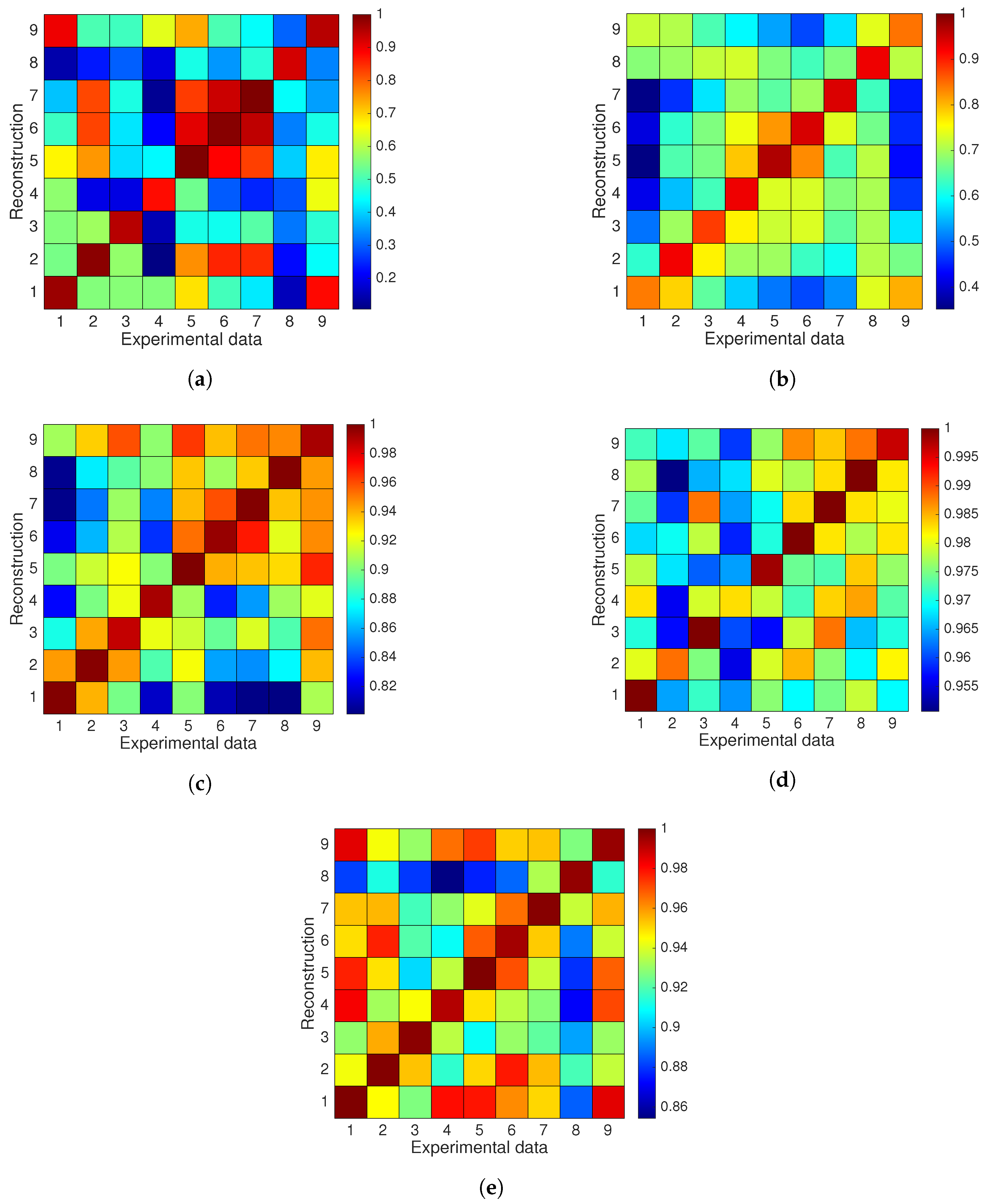
4.2. Reconstruction of Squeal Noise and Comparison with Experiments

The acoustic field reconstruction based on the method proposed in Section 4.1 is applied to validate its effectiveness for reproducing the characterization of squeal noise at the location of the antenna microphones. These numerical calculations for the reconstruction of the radiated field are compared with the direct pressure measurements provided by the antenna microphones (by considering the main frequencies of interest, as previously stated in Section 3.2) in order to validate the assumptions of the method adopted, in particular the plane wave and free field assumptions. We notice that the Tikhonov regularization proposed in Equation (4) prevents the reconstruction from exactly matching the experiments, since we use the $\epsilon$ value recommended by Hald [31], which is assumed to be well-suited to the method proposed.

Figure 11, Figure 12, Figure 13, Figure 14 and Figure 15 show the reconstruction of the acoustic patterns for frequencies $f_1=610$ Hz, $f_2=1220$ Hz, $f_3=1830$ Hz, $f_4=2440$ Hz and $f_5=3050$ Hz, respectively. The reconstruction of the radiated acoustic field is proposed by examining nine frames displayed evenly over time by considering one period of disc revolution (to be compared to the previous radiated acoustic fields obtained by the direct pressure measurements of the microphones antenna shown in the first nine subfigures of Figure 6, Figure 7, Figure 8, Figure 9 and Figure 10, respectively).

These show that the evolution of the radiated field is repeatable over several rounds and that a nine-frame discretization is sufficient to provide an appropriate representation of the temporal evolution of the acoustic pattern for both level and directivity. Whatever the frequency considered, it can be seen very clearly that the different patterns and their evolution in terms of both directivity and level are very well reproduced.

In order to quantify the error between the direct pressure measurements and the reconstructed acoustic field for each frequency of interest in the squeal noise, the well-known correlation coefficient is used. Considering two families of sequences defined by $\mathbf{A}=[{\mathbf{A}}_1,{\mathbf{A}}_2,\dots ,{\mathbf{A}}_N]$ and $\mathbf{B}=[{\mathbf{B}}_1,{\mathbf{B}}_2,\dots ,{\mathbf{B}}_N]$, the associated correlation coefficients can be represented in matrix $\mathbf{R}$ according to the following formula:

$${\mathbf{R}}_{mn}=\frac{{\left|{\left({\mathbf{A}}_n-{\overline{\mathbf{A}}}_n\right)}^T.\left({\mathbf{B}}_m-{\overline{\mathbf{B}}}_m\right)\right|}^2}{∥{\mathbf{A}}_n^T-{\overline{\mathbf{A}}}_n∥.∥{\mathbf{B}}_m^T-{\overline{\mathbf{B}}}_m∥},$$

(14)

where ${\overline{\mathbf{A}}}_{\mathbf{n}}$ and ${\overline{\mathbf{B}}}_{\mathbf{m}}$ are the mean values of vectors ${\mathbf{A}}_n$ and ${\mathbf{B}}_m$. ${\mathbf{R}}_{mn}$ is called the scalar correlation coefficient corresponding to the nth sequence of $\mathbf{A}$ and the mth sequence of $\mathbf{B}$. Each correlation coefficient returns a scalar value between 0 and 1. If ${\mathbf{R}}_{mn}$ is close to one, this means that there is a very good correlation between the two sequences, while a value close to zero corresponds to a bad correlation. It should be noted that in the present case, vectors ${\mathbf{A}}_i$ and ${\mathbf{B}}_i$ (with $i=1,\dots ,N$) correspond to the data for one specific frequency of interest, obtained from the direct pressure measurements and the reconstructed acoustic field for the 117 microphones (i.e., the size of vectors ${\mathbf{A}}_i$ and ${\mathbf{B}}_i$ is $117\times 1$). Moreover, as explained previously, the evolution of the acoustic radiated field patterns for one disc revolution is discretized by using nine frames, thus the scalar N is equal to nine (i.e., the size of matrices $\mathbf{A}$ and $\mathbf{B}$ is $117\times 9$). The results provided in Figure 16 offer the scalar correlation coefficient $R_{mn}$ (for $m=1,\dots ,9$ and $n=1,\dots ,9$) between the direct pressure measurements and the reconstructed acoustic field for each frequency of interest and by considering the nine sequences per disc revolution. Thus, the diagonal terms provide information on the quality of the method for reconstructing the acoustic field and its evolution over one revolution of the disc, while the extra-diagonal terms provide only information on the similarity for the two selected samples (i.e., one experimental item of data from the mth sequence and one reconstructed field from the nth sequence with $n\ne m$) considered at two different times. By analyzing the results proposed in Figure 16, it can first be mentioned that the effectiveness of the reconstruction method is validated since all the diagonal terms, whatever the frequency considered, are composed of values very close to one. This shows, unambiguously, that for all 117 microphones, the evolution of the reconstructed radiated field is in very good agreement with the evolution of the measured acoustic field and thus that the reconstruction of the squeal noise by the method proposed provides an appropriate representation of the temporal evolution of the acoustic pattern for both level and directivity. In addition, due to the fact that the reconstructed radiated field and the direct acoustic data measurements are similar over the nine discrestized times, the extra-diagonal terms of ${\mathbf{R}}_{mn}$ can be used to quantify the temporal evolution, per one revolution of the disc, for the radiated acoustic pattern for both level and directivity for the five frequencies of interest. Thus, if we consider the results associated with the first two frequencies more specifically (see Figure 16a for $f_1=610$ Hz and Figure 16b for $f_2=1220$ Hz), the values of the extra-diagonal terms indicate a temporal evolution of the sound field pattern over one revolution of the disc. This is in very good agreement with the experimental observations proposed in Section 3.2 which indicate that the variation of the radiated acoustic fields in terms of level and directivity can be linked to the rotation speed of the disc. Moreover, the fact that this phenomenon is considered to be greater for $f_1$ is also reflected in the values of the extra-diagonal coefficients ${\mathbf{R}}_{mn}$ indicating values closer to zero for frequency $f_1$. This points to non-similarity between two quantities taken at different temporal instants, characterizing a stronger temporal evolution of the acoustic radiated field. Furthermore, the extra-diagonal terms for the last three frequencies of interest all remain above 0.8 (see Figure 16c for $f_3=1830$ Hz, Figure 16d for $f_4=2440$ Hz and Figure 16e for $f_5=3050$ Hz). This indicates that the acoustic pattern changes very little over time. These results are again in very good agreement with the observations proposed previously in Section 3.2. To further the analysis, we note that for frequency $f_4$, the acoustic pattern can be considered as constant versus the rotation of the disc due to the fact that the correlation coefficients are always above 0.95 (see Figure 16d).

Table 2. Uses of the indicator ${\mathbf{R}}_{mn}$ to characterize the evolution of the acoustic field versus time for one disc revolution.

	${\mathit{f}}_1$	${\mathit{f}}_2$	${\mathit{f}}_3$	${\mathit{f}}_4$	${\mathit{f}}_5$
${\displaystyle \underset{m}{min}\left[{\mathbf{R}}_{mm}\right]}$	0.85	0.8	0.99	0.98	0.99
${\displaystyle \underset{(m,n)}{min}\left[{\mathbf{R}}_{mn}\right]}$	0.07	0.37	0.81	0.95	0.86
Evolution vs. time	very strong	strong	low	none	low

groups these observations and highlights the temporal evolution of the acoustic patterns corresponding to frequencies $f_1$ and $f_2$, and the temporal constancy of the patterns linked to frequencies $f_3$, $f_4$ and $f_5$. ${\displaystyle \underset{m}{min}\left[{\mathbf{R}}_{mm}\right]}$ corresponds to the minimum value observed for the diagonal terms. This allows validating the relevance of the method for reconstructing the acoustic radiated field measured. If all the values are close to one for all the frequencies of interest, this means that the method implemented can be used to reconstruct the evolution of the acoustic radiated field during squeal events with effectiveness and robustness and thus achieve a robust representation of 3D acoustic models for understanding of acoustic squealing events, which is discussed in the next section. ${\displaystyle \underset{(m,n)}{min}\left[{\mathbf{R}}_{mn}\right]}$ highlights the minimal value of the extra-diagonal terms. As explained previously, if this value is small, the acoustic pattern evolves over time per disc revolution. This is therefore an interesting indicator for quantifying a more or less significant fluctuation of the acoustic radiated field over time.

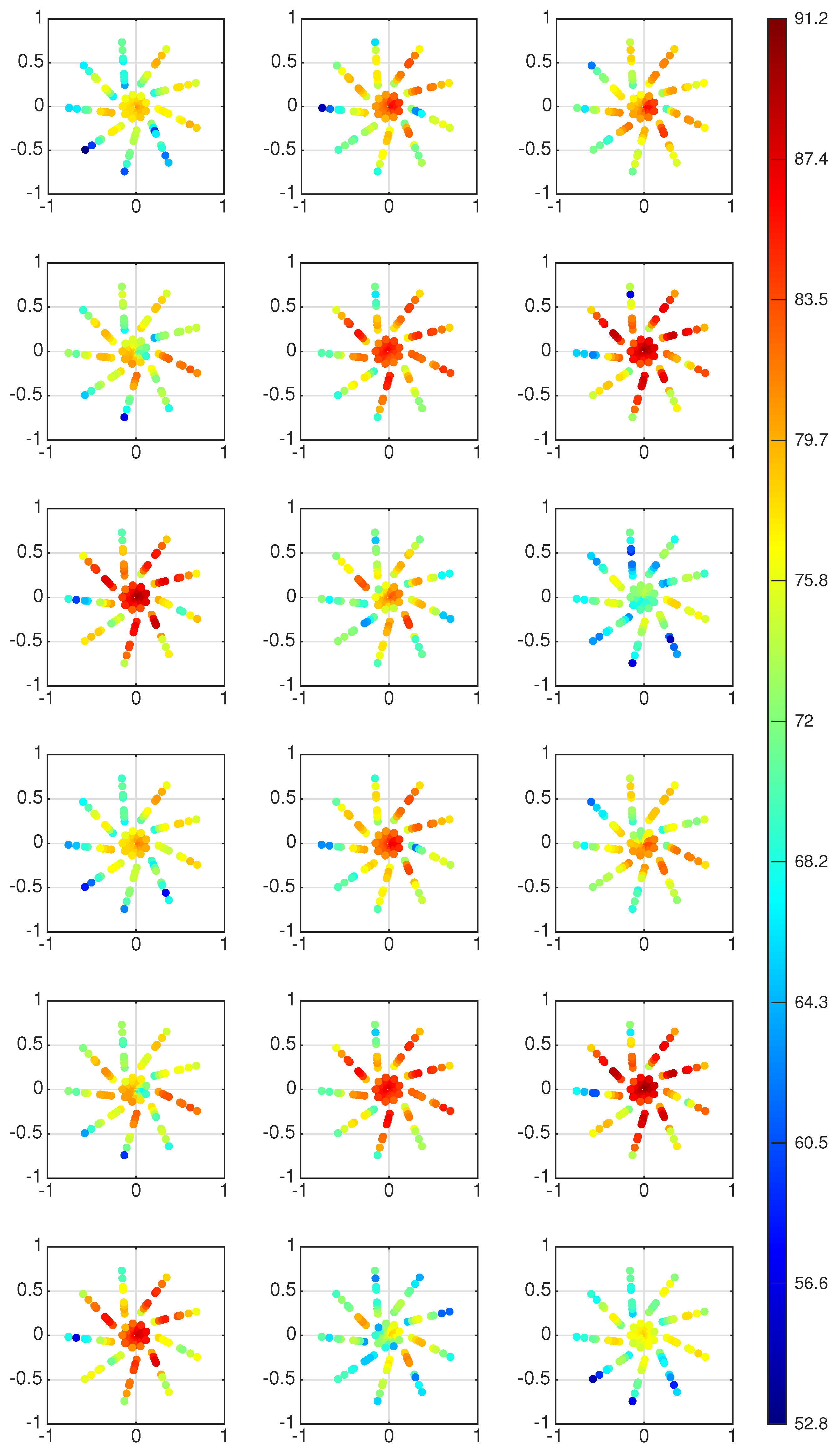
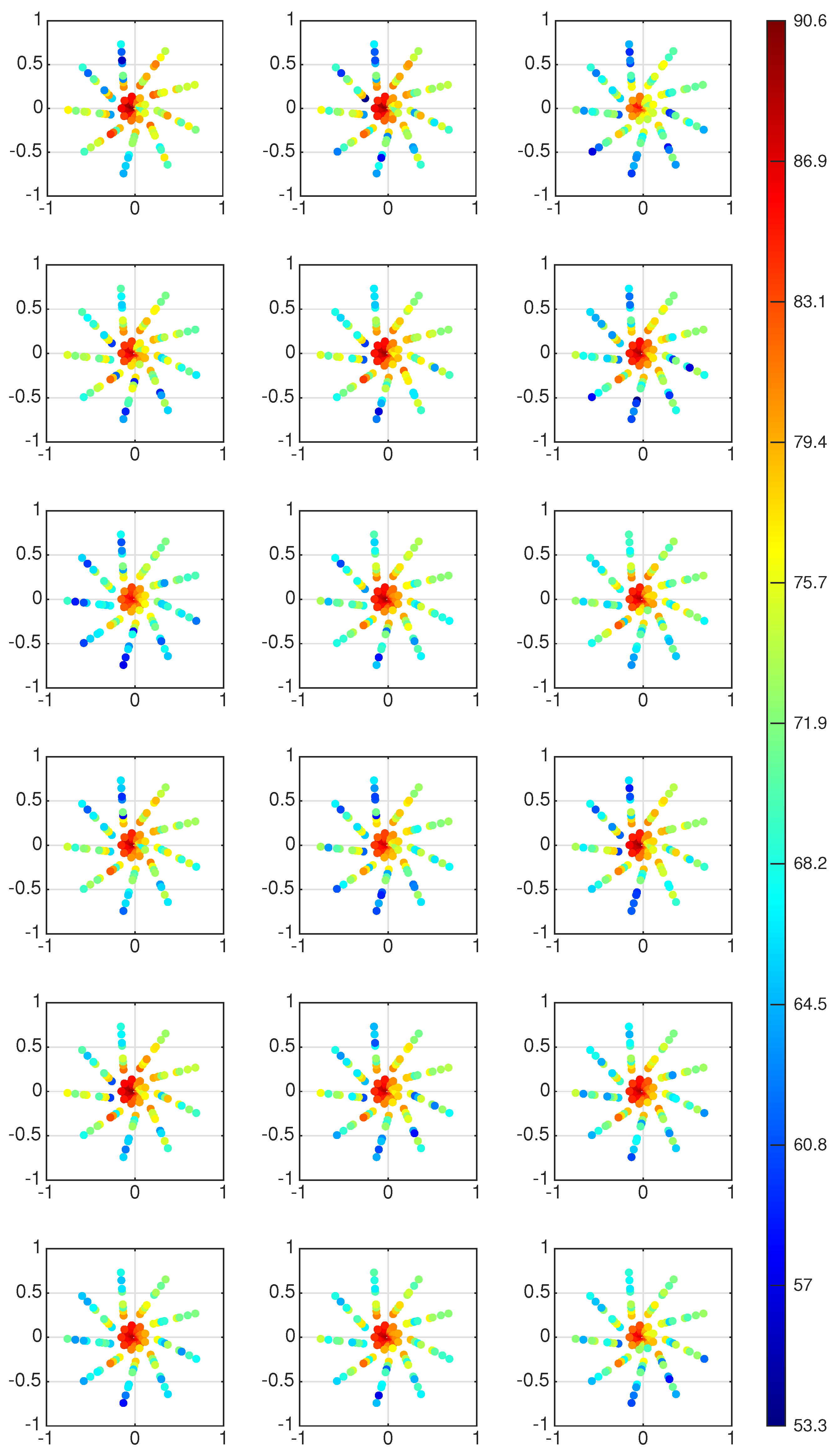
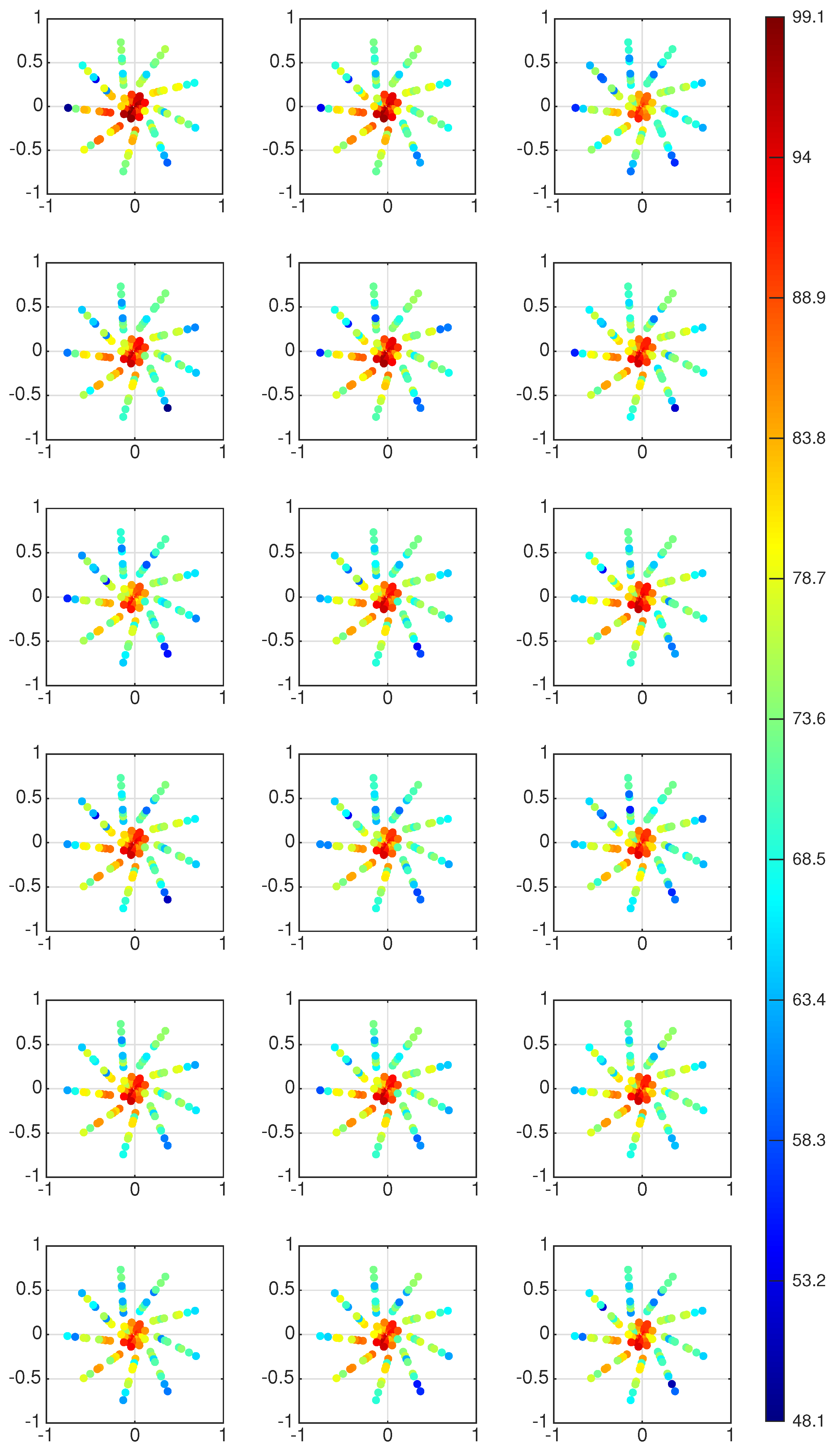
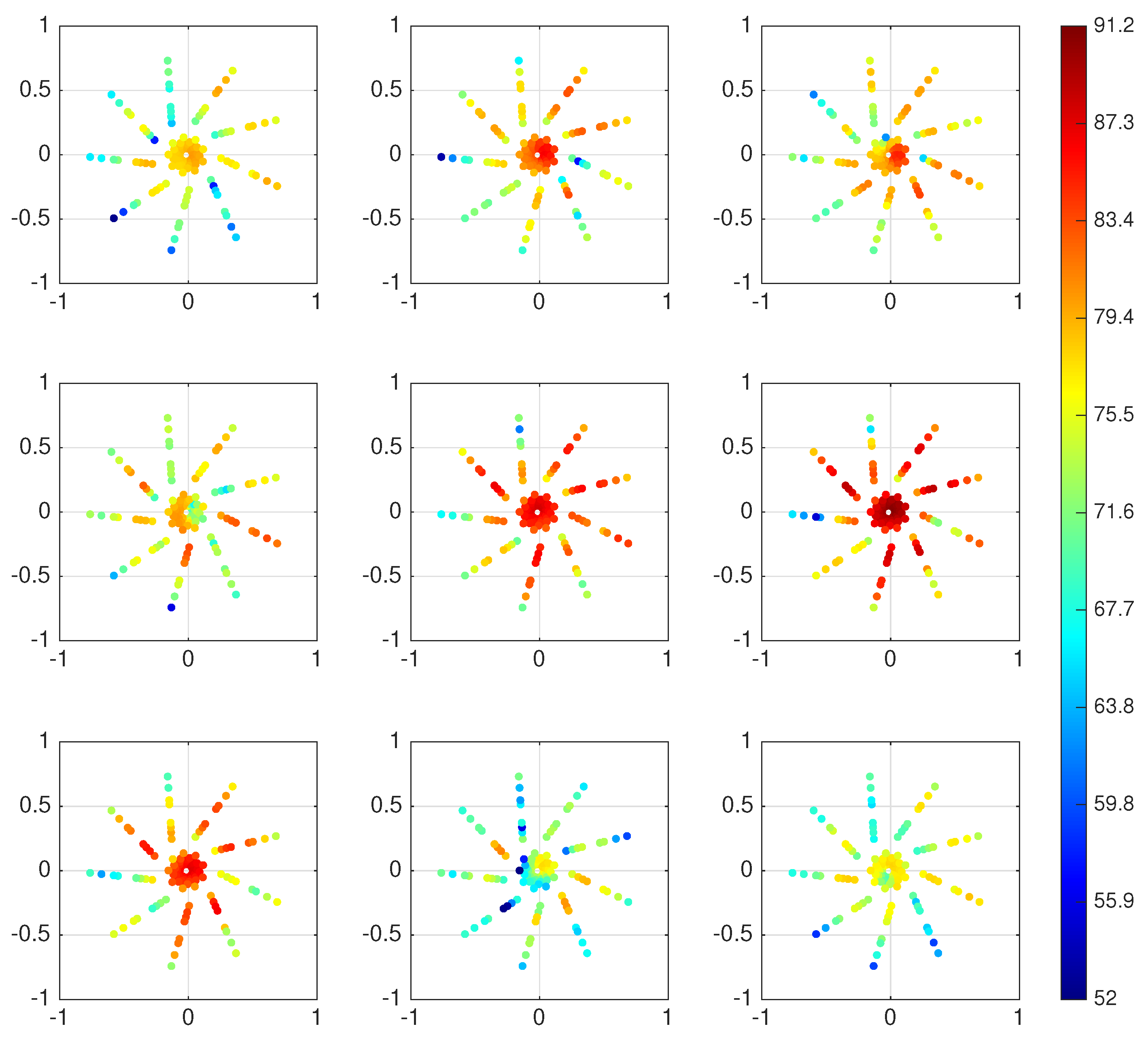
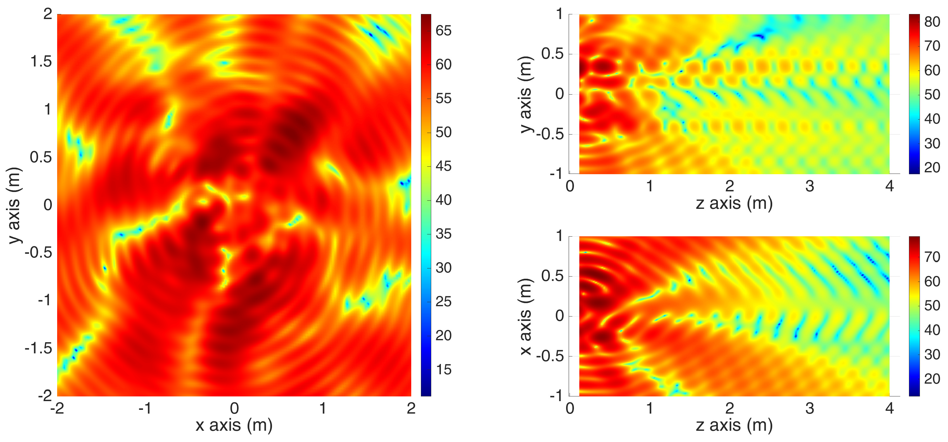
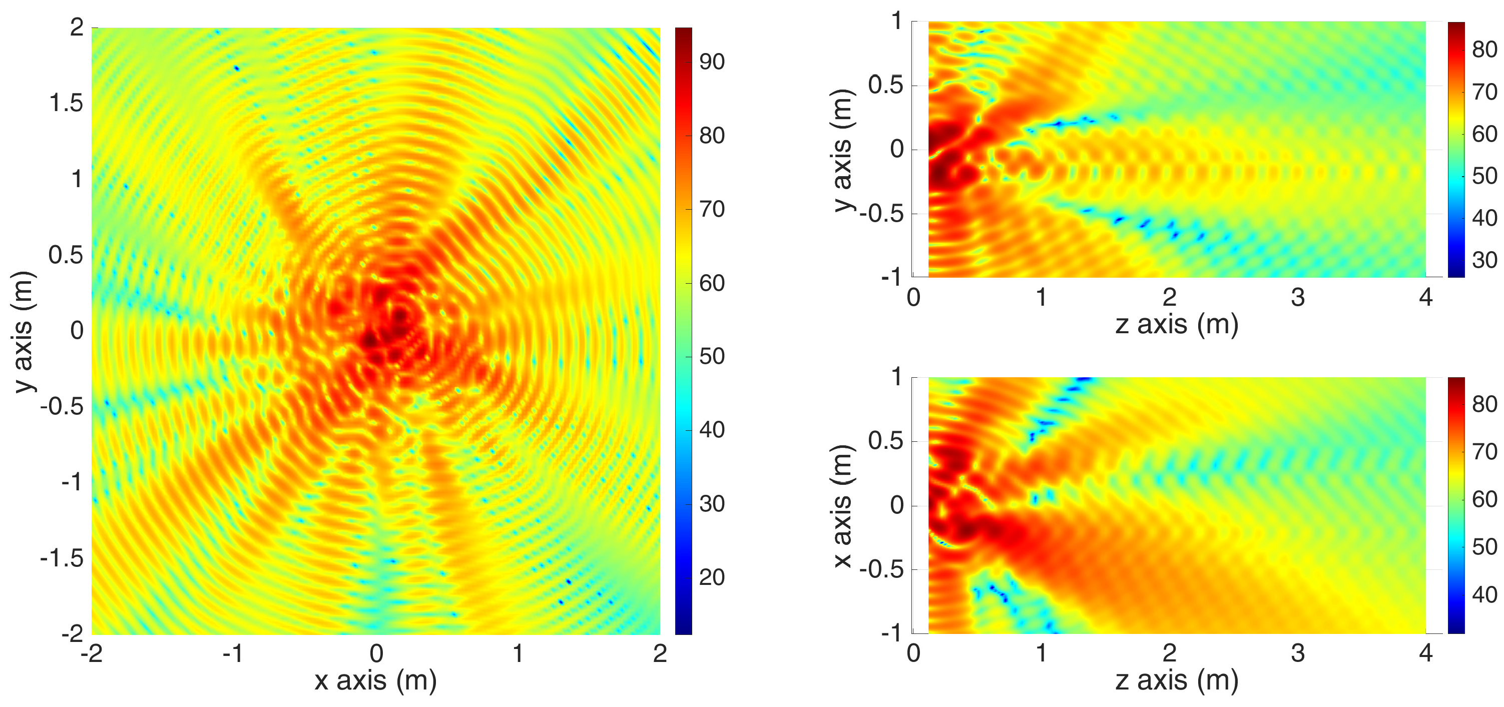
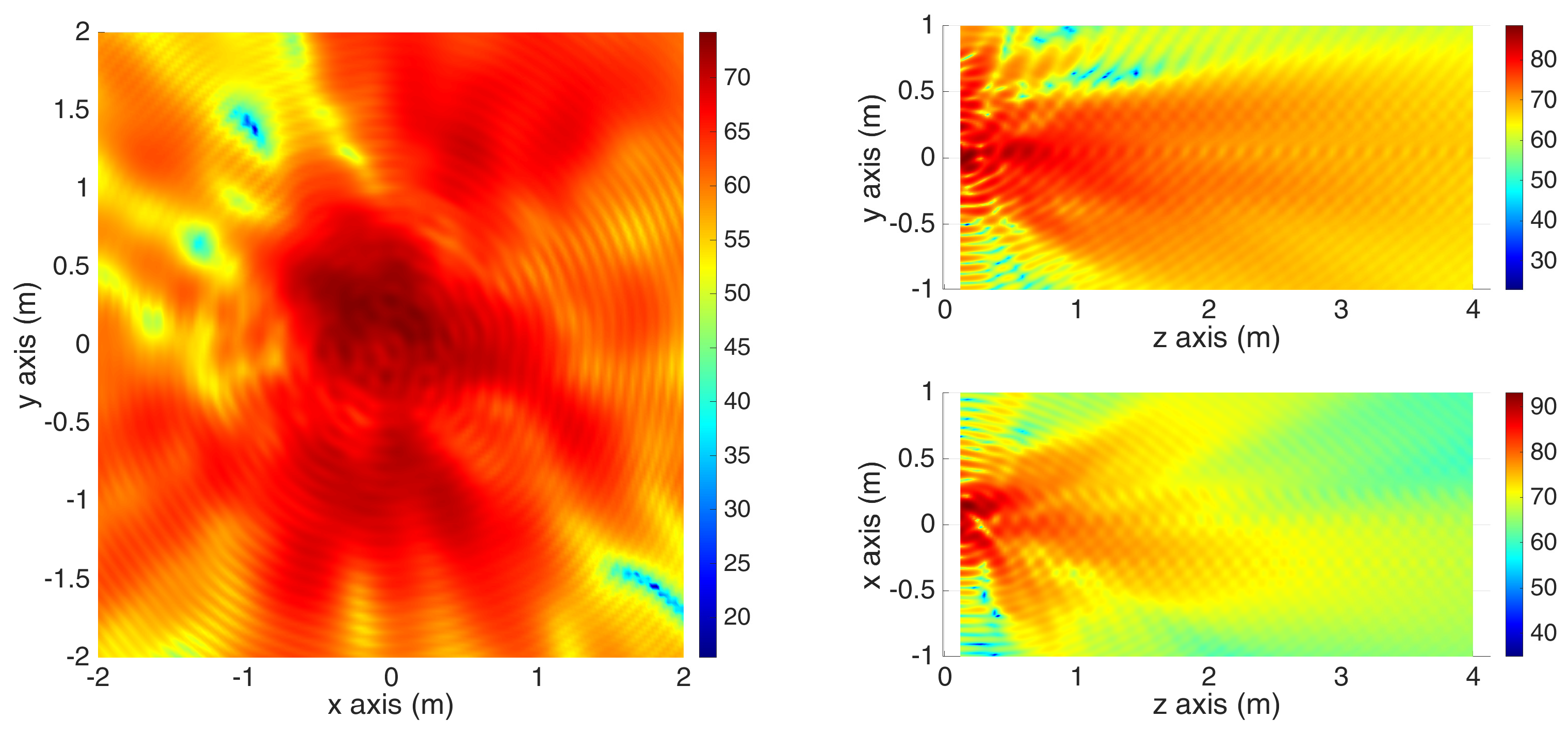
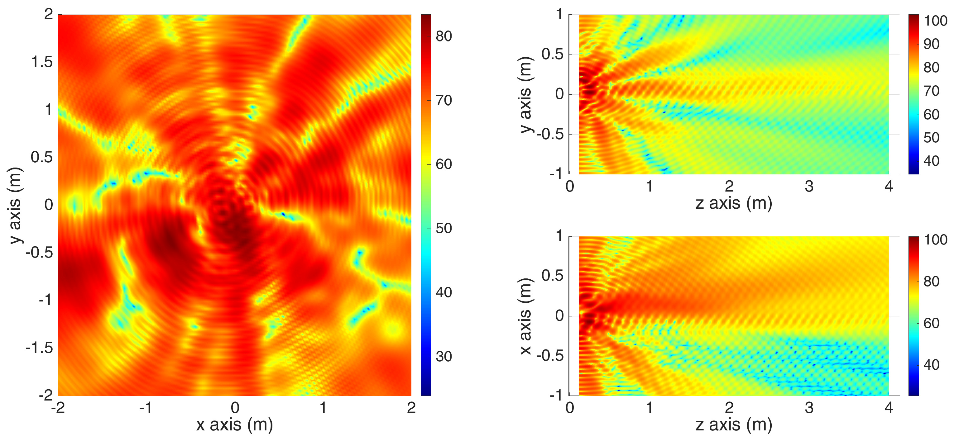
4.3. 3D Reconstruction of Squeal Noise

As previously discussed in Section 4.2, the acoustic field reconstruction method is proposed to reproduce the squeal noise of the brake system subjected to friction-induced vibration. Its validation is obtained by comparing the estimated acoustic field and the data measurements at the location of the 117 microphones. In the following section, we focus on the ability to reconstruct the radiated sound field anywhere in the space surrounding the braking system (downstream of the antenna). This should provide a more accurate pattern of the acoustic radiated field and thus provide further insights into the 3D radiated acoustic field during squeal events. The main assumption of the 3D sound field reconstruction calculations is that the previous results obtained in the pressure field reconstruction at the measurement points make it possible to extend the reconstruction method to the whole space.

More specifically, regarding the 3D sound field reconstruction strategy, it is carried out by defining different 2D planes of interest, on which the propagation of the acoustic radiated field is estimated. In order to achieve this objective, the reconstructed acoustic field is calculated at $N_P$ specific points on the selected 2D plane. Then, the calculation of the pressure field at the $N_P$ assessment points according to the measurements of the 117 microphones is performed as explained in Section 4.1. To obtain a precise representation of the reconstructed radiated field, $N_P$ is chosen to be equal to 150.

More specifically, to illustrate the results based on this 3D reconstruction approach, three analyses are carried out on selected specific 2D planes of interest:

• one section defined along the plane $(0,x,y)$ and located at $z=2$ m. These results correspond to the reconstruction of the acoustic noise field that is relatively distant from the experimental measurements of the antenna microphones;
• one section defined along the vertical plane $(0,z,y)$ and passing through the center of the disc. This provides a visualization of the acoustic propagation in the vertical plane over a distance of 0 to 4 m with respect to the direction normal to the plane of the brake disc (along z-axis);
• one section defined along the horizontal plane $(0,z,x)$ and passing through the center of the disc (i.e., orthogonal to the chosen vertical plane $(0,z,y)$). This offers a complementary representation to the previous visualization of the propagation of the acoustic field over a distance of 0 to 4 m.

Figure 17, Figure 18, Figure 19, Figure 20 and Figure 21 show the propagation of the acoustic radiated field during squeal events (at the fixed time $t=24$ s) for the five main frequencies of interest, respectively. This offers an overview of the acoustic levels and directivity involved for each frequency of interest. However, given the potential variability of the acoustic pattern as a function of time (as discussed previously in Section 2), it is advisable to treat these results with caution, as they are a reflection of a single reconstruction of the acoustic field for one specific time (i.e., $t=24$ s). However, these results are sufficient to provide a number of conclusions regarding the proposed reconstruction.

The representations of the squeal noise in the $(0,x,y)$ plane show that the acoustic pattern radiated at $z=2$ m is different depending on the frequency considered, both in level and directivity. Moreover, although for frequencies $f_1=610$ Hz and $f_3=1830$ Hz a relatively homogeneous and centered directivity is observed, this is not the same for the three other frequencies which give rise to a more erratic acoustic pattern. It can also be noted that this radiated field propagation diagram becomes more complex when considering the five frequencies of interest in increasing order, which is consistent with the evolution of the associated wavelengths. Considering the representations in the two planes, $(0,z,y)$ and $(0,z,x)$, the results obtained show a dissymmetry of the propagation of the radiated acoustic field which can be explained by imperfect absorption conditions on the one hand and by the non-symmetry of the disc/caliper system studied on the other. However, it can be clearly seen that this observed dissymmetry remains relatively moderate for the overall evolution of the acoustic field propagated. Unsurprisingly, it can also be noted that the source of the radiated acoustic noise for the five frequencies of interest is located at the brake system position, with a decrease in the sound level when moving away from the brake disc.

In conclusion, all of these results illustrate that the proposed reconstruction method provides an overview of the three-dimensional radiated acoustic field resulting from the self-excited vibration during braking, thus providing physically interesting information on the acoustic behavior associated with the squeal phenomenon.

5. Conclusions

This study provides insight into the acoustic radiation generated during the squeal phenomenon in a brake system. Firstly, the acoustic phenomena during squeal events are investigated and, more specifically, their characteristics versus squeal frequencies are determined by analyzing the acoustic pattern (in terms of both directivity and sound level) per disc revolution. The reproducibility of the radiated acoustic field of each squeal frequency is highlighted for a given set of operational parameters. The squeal noise of the braking system is mainly characterized by a fundamental frequency and its harmonic components. Frequency contributions of lower acoustic intensity are also detectable. The squeal frequencies detected via acoustic measurements are similar to the squeal frequencies previously observed on vibrations during braking tests, which unambiguously demonstrates the potential links between the emergence of friction-induced vibrations and the squeal noise in far field. It is also shown that the radiated acoustic field emanating from each squeal frequency has its own directivity and intensity characteristics with eventual evolution per revolution of the disc.

In addition, a method for reconstructing the acoustic field radiated in all the surrounding space is implemented. This approach is validated by reconstructing the pressure field at the location of the 117 measurement points of the microphone antenna and using a similarity criterion that allows verifying the correlation between the measured data and the output data of the reconstruction of the measurement points. We note that this similarity criterion is also used to highlight the temporal evolution of the acoustic pattern specific to each frequency of the squeal noise and thus obtain understanding of the radiated acoustic patterns as a function of disc rotation. Finally, the method implemented is applied to illustrate the method’s capability of reconstructing the radiated acoustic field everywhere in the surrounding space of the brake system.

It would be interesting in the next step of the study to use the pressure measurements to identify, locate and characterize the vibratory sources responsible for acoustic radiation and hence the problem of friction-induced vibration. This would provide additional insight into the problem of the origin of squeal noise in brake systems.

References

1. Papinniemi, A.; Lai, J.; Zhao, J.; Loader, L. Brake squeal: A literature review. Appl. Acoust. 2002, 63, 391–400. [Google Scholar] [CrossRef]
2. Kindkaid, N.; O’Reilly, O.; Papadopoulos, P. Automative disc brake squeal. J. Sound Vib. 2003, 267, 105–166. [Google Scholar] [CrossRef]
3. Ouyang, H.; Nack, W.; Yuan, Y.; Chen, F. Numerical analysis of automative disc brake squeal: A review. Int. J. Veh. Noise Vib. 2005, 1, 207–231. [Google Scholar] [CrossRef]
4. Ibrahim, R. Friction-induced vibration, chatter, squeal, and chaos part 1: Mechanics of contact and friction. Appl. Mech. Rev. 1994, 47, 209–226. [Google Scholar] [CrossRef]
5. Ibrahim, R. Friction-induced vibration, chatter, squeal, and chaos part 2: Dynamics and modeling. Appl. Mech. Rev. 1994, 47, 227–263. [Google Scholar] [CrossRef]
6. Oberst, S.; Lai, J.C.S. Statistical analysis of brake squeal noise. J. Sound Vib. 2011, 330, 2978–2994. [Google Scholar] [CrossRef]
7. Tison, T.; Massa, F.; Turpin, I.; Nunes, R.F. Improvement in the predictivity of squeal simulations: Uncertainty and robustness. J. Sound Vib. 2014, 333, 3394–3412. [Google Scholar] [CrossRef]
8. Nobari, A.; Ouyang, H.; Bannister, P. Uncertainty quantification of squeal instability via surrogate modelling. Mech. Syst. Signal Process. 2015, 60–61, 887–908. [Google Scholar] [CrossRef]
9. Renault, A.; Massa, F.; Lallemand, B.; Tison, T. Experimental investigations for uncertainty quantification in brake squeal analysis. J. Sound Vib. 2016, 367, 37–55. [Google Scholar] [CrossRef]
10. Poletto, J.; Neis, P.; Ferreira, N.; Masotti, D.; Matozo, L. An experimental analysis of the methods for brake squeal quantification. Appl. Acoust. 2017, 122, 107–112. [Google Scholar] [CrossRef]
11. Denimal, E.; Sinou, J.J.; Nacivet, S. Influence of structural modifications of automotive brake systems for squeal events with kriging meta-modelling method. J. Sound Vib. 2019, 463, 114938. [Google Scholar] [CrossRef]
12. Chevillot, F.; Sinou, J.J.; Hardouin, N.; Jézéquel, L. Simulations and experiments of a nonlinear aircraft braking system with physical dispersion. J. Vib. Acoust. 2010, 132, 041010. [Google Scholar] [CrossRef]
13. Sinou, J.J.; Dereure, O.; Mazet, G.B.; Thouverez, F.; Jézéquel, L. Friction Induced Vibration for an Aircraft Brake System. Part I: Experimental approach and Stability Analysis. Int. J. Mech. Sci. 2006, 48, 536–554. [Google Scholar] [CrossRef]
14. Panier, S.; Dufrénoy, P.; Weichert, D. An experimental investigation of hot spots in railway disc brakes. Wear 2004, 256, 764–773. [Google Scholar] [CrossRef]
15. Lorang, X.; Foy-Margiocchi, F.; Nguyen, Q.; Gautier, P. TGV disc brake squeal. J. Sound Vib. 2006, 293, 735–746. [Google Scholar] [CrossRef]
16. Majcherczak, D.; Dufrénoy, P.; Berthier, Y. Tribological, thermal and mechanical coupling aspects of the dry sliding contact. Tribol. Int. 2007, 40, 834–843. [Google Scholar] [CrossRef]
17. Sinou, J.J.; Loyer, A.; Chiello, O.; Mogenier, G.; Lorang, X.; Cocheteux, F.; Bellaj, S. A global strategy based on experiments and simulations for squeal prediction on industrial railway brakes. J. Sound Vib. 2013, 332, 5068–5085. [Google Scholar] [CrossRef]
18. Massi, F.; Giannini, O.; Baillet, L. Brake squeal as dynamic instability: An experimental investigation. J. Acoust. Soc. Am. 2006, 120, 1388–1398. [Google Scholar] [CrossRef]
19. Massi, F.; Baillet, L.; Giannini, O.; Sestieri, A. Brake squeal: Linear and nonlinear numerical approaches. Mech. Syst. Signal Process. 2007, 21, 2374–2393. [Google Scholar] [CrossRef]
20. Akay, A.; Giannini, O.; Massi, F.; Sestieri, A. Disc brake squeal characterization through simplified test rigs. Mech. Syst. Signal Process. 2009, 23, 2590–2607. [Google Scholar] [CrossRef]
21. Butlin, T.; Woodhouse, J. A systematic experimental study of squeal initiation. J. Sound Vib. 2011, 330, 5077–5095. [Google Scholar] [CrossRef]
22. Kado, N.; Sato, N.; Tadokoro, C.; Skarolek, A.; Nakano, K. Effect of yaw angle misalignment on brake noise and brake time in a pad-on-disc-type apparatus with unidirectional compliance for pad support. Tribol. Int. 2014, 78, 4–46. [Google Scholar] [CrossRef]
23. Butlin, T.; Woodhouse, J. Friction-induced vibration: Model development and comparison with large-scale experimental tests. J. Sound Vib. 2013, 332, 5302–5321. [Google Scholar] [CrossRef]
24. Bonnay, K.; Magnier, V.; Brunel, J.; Dufrénoy, P.; Saxcé, G.D. Influence of geometry imperfections on squeal noise linked to mode lock-in. Int. J. Solids Struct. 2015, 75–76, 99–108. [Google Scholar] [CrossRef]
25. Sinou, J.J.; Lenoir, D.; Besset, S.; Gillot, F. Squeal analysis based on the laboratory experimental bench “Friction-Induced Vibration and noisE at École Centrale de Lyon” (FIVEECL). Mech. Syst. Signal Process. 2019, 119, 561–588. [Google Scholar] [CrossRef]
26. Lenoir, D.; Besset, S.; Sinou, J.J. Transient vibro-acoustic analysis of squeal events based on the experimental bench FIVE@ECL. Appl. Acoust. 2020, 165, 107286. [Google Scholar] [CrossRef]
27. Sinou, J.J.; Besset, S.; Lenoir, D. Some unexpected thermal effects on squeal events observed on the experimental bench FIVE@ECL. Mech. Syst. Signal Process. 2021, 160, 107867. [Google Scholar] [CrossRef]
28. Hendricx, W.; Garesci, F.; Pezzutto, A.; Van der Auweraer, H. Experimental and numerical modelling of friction induced noise in disc brakes. SAE Trans. 2002, 111, 1566–1571. [Google Scholar] [CrossRef]
29. Flint, J.; Hald, J. Traveling Waves in Squealing Disc Brakes Measured with Acoustic Holography. Sae Tech. Pap. 2003. [Google Scholar] [CrossRef]
30. Fieldhouse, J.; Newcomb, T. Double pulsed holography used to investigate noisy brakes. Opt. Lasers Eng. 1996, 25, 455–494. [Google Scholar] [CrossRef]
31. Hald, J. Basic theory and properties of statistically optimized near-field acoustical holography. J. Acoust. Soc. Am. 2009, 125, 2105–2120. [Google Scholar] [CrossRef]
32. Wang, Z.; Wu, S.F. Helmholtz equation-least-squares method for reconstructing the acoustic pressure field. J. Acoust. Soc. Am. 1997, 102, 2020. [Google Scholar] [CrossRef]
33. Wu, S.F. On reconstruction of acoustic fields using the Helmholtz equation least squares method. J. Acoust. Soc. Am. 2000, 107, 2511. [Google Scholar] [CrossRef] [PubMed]
34. Williams, E.G.; Maynard, J.D.; Skudrzyk, E.J. Sound source reconstruction using a microphone array. J. Acoust. Soc. Am. 1980, 68, 340. [Google Scholar] [CrossRef]
35. Maynard, J.D.; Williams, E.G.; Lee, Y. Nearfield acoustic holography: I. Theory of generalized holography and the development of NAH. J. Acoust. Soc. Am. 1985, 78, 1395. [Google Scholar] [CrossRef]
36. Saijyou, K.; Yoshikawa, S. Reduction methods of the reconstruction error for large-scale implementation of near-field acoustical holography. J. Acoust. Soc. Am. 2001, 110, 2007. [Google Scholar] [CrossRef] [PubMed]
37. Gomes, J.; Hansen, P. A study on regularization parameter choice in Near-field Acoustical Holography. In Proceedings of the Acoustics’08, Paris, France, 30 June–4 July 2008; pp. 2875–2880. [Google Scholar] [CrossRef]
38. Hald, J. Patch Near-field Acoustical Holography Using a New Statistically Optimal Method. In Proceedings of the PInter-Noise, Seogwipo, Republic of Korea, 25–28 August 2003. [Google Scholar] [CrossRef]
39. Hald, J. Patch holography in cabin environments using a two-layer handheld array with an extended SONAH algorithm. In Proceedings of the Euronoise, Tampere, Finland, 30 May–1 June 2006. [Google Scholar] [CrossRef]
Figure 1. Experimental bench FIVE@ECL. (a) Braking system; (b) Digital microphone antenna.
Applsci 13 12246 g001
Figure 2. Protocol for one braking test and evolution of the operational parameters.
Applsci 13 12246 g002
Figure 3. Positioning of the 117 microphones in the plane of the digital microphone antenna.
Applsci 13 12246 g003
Figure 4. Decay of the time signal as a function of the distance from the braking system.
Applsci 13 12246 g004
Figure 5. Spectrogram for one microphone of the digital antenna (dB).
Applsci 13 12246 g005
Figure 6. Evolution of the acoustic radiation for all the microphones of the digital antenna at f 1 = 610 Hz over two periods of disc revolution (in dB SPL)—to be read from left to right, top to bottom.
Applsci 13 12246 g006
Figure 7. Evolution of the acoustic radiation for all the microphones of the digital antenna at f 2 = 1220 Hz over two periods of disc revolution (in dB SPL)—to be read from left to right, top to bottom.
Applsci 13 12246 g007
Figure 8. Evolution of acoustic radiation for all the microphones of the digital antenna at f 3 = 1830 Hz over two periods of disc revolution (in dB SPL)—to be read from left to right, top to bottom.
Applsci 13 12246 g008
Figure 9. Evolution of acoustic radiation for all the microphones of the digital antenna at f 4 = 2440 Hz over two periods of disc revolution (in dB SPL)—to be read from left to right, top to bottom.
Applsci 13 12246 g009
Figure 10. Evolution of acoustic radiation for all the microphones of the digital antenna at f 5 = 3050 Hz over two periods of disc revolution (in dB SPL)—to be read from left to right, top to bottom.
Applsci 13 12246 g010
Figure 11. Reconstruction of the radiated field for f 1 = 610 Hz and its temporal evolution for one disc revolution (to be compared with Figure 6)—to be read from left to right, top to bottom.
Applsci 13 12246 g011
Figure 12. Reconstruction of the radiated field for f 2 = 1220 Hz and its temporal evolution for one disc revolution (to be compared with Figure 7)—to be read from left to right, top to bottom.
Applsci 13 12246 g012
Figure 13. Reconstruction of the radiated field for f 3 = 1830 Hz and its temporal evolution for one disc revolution (to be compared with Figure 8)—to be read from left to right, top to bottom.
Applsci 13 12246 g013
Figure 14. Reconstruction of the radiated field for f 4 = 2440 Hz and its temporal evolution for one disc revolution (to be compared with Figure 9)—to be read from left to right, top to bottom.
Applsci 13 12246 g014
Figure 15. Reconstruction of the radiated field for f 5 = 3050 Hz and its temporal evolution for one disc revolution (to be compared with Figure 10)—to be read from left to right, top to bottom.
Applsci 13 12246 g015
Figure 16. Correlation coefficient R m n between the direct pressure measurements and the reconstructed acoustic field for each frequency of interest and by considering sequences of nine frames per disc revolution. (a) f 1 = 610 Hz; (b) f 2 = 1220 Hz; (c) f 3 = 1830 Hz; (d) f 4 = 2440 Hz; (e) f 5 = 3050 Hz.
Applsci 13 12246 g016
Figure 17. 3D reconstruction of the radiated acoustic field for f 1 = 610 Hz and at t = 24 s.
Applsci 13 12246 g017
Figure 18. 3D reconstruction of the radiated acoustic field for f 2 = 1220 Hz and at t = 24 s.
Applsci 13 12246 g018
Figure 19. 3D reconstruction of the radiated acoustic field for f 3 = 1830 Hz and at t = 24 s.
Applsci 13 12246 g019
Figure 20. 3D reconstruction of the radiated acoustic field for f 4 = 2440 Hz and at t = 24 s.
Applsci 13 12246 g020
Figure 21. 3D reconstruction of the radiated acoustic field for f 5 = 3050 Hz and at t = 24 s.
Applsci 13 12246 g021