Nonlinear Controller for an Inverted Pendulum Using the Trigonometric Function

Abstract

In this paper, a nonlinear controller (TR) for an inverted pendulum using the trigonometric function is presented. The TR controller is a new proposal, which is represented by a simple mathematical formula. TR operation does not require complex calculations, so it can be applied even to the simplest microcontrollers. Tuning the TR controller is very simple, and the range of stable operation is very wide. Simulation tests of the TR controller showed that the controller is effective even for deviations exceeding 50${}^{\circ }$. The TR controller tests were compared to the results of a PID controller. The TR controller is designed to stabilise an inverted pendulum in the equilibrium point, a state in which the pendulum is in a upright position. Stabilisation for other deflection-angle set points was not taken into account. During the research, steps were taken to simulate phenomena characteristic of real solutions. An inertial block and a disturbance were introduced into the test system. Despite the introduced difficulties, the TR controller effectively stabilised the pendulum without the need to retune the controller settings. Consequently, the TR controller is an attractive alternative to previously applied solutions for the stabilisation of an inverted pendulum.

1. Introduction

The inverted pendulum is used in modelling and research in various fields of science and engineering due to its complexity and interesting properties. It is particularly used in robotics, where stabilisation of the inverted pendulum is one of the primary tasks. Robots equipped with inverted pendulums must have controllers to maintain their balance in order to move on uneven terrain. By using such models, they can even overcome such significant differences in levels as stairs [1,2,3,4]. The problem of stabilising robots and controlling them with the desired accuracy and resistance to interference is an issue widely discussed in the literature. The inverted pendulum model is applied to different types of robots, including single-wheeled or two-wheeled robots [5,6].

Outside of robotics, the inverted pendulum model is used in the stabilisation of vehicles such as bicycles, motorbikes or cars. The inverted pendulum is also used to analyse human behaviour in a quiet standing position [7]. This tool allows for the study of human balance and response to different stimuli. In astronautics, the inverted pendulum model is used to simulate the behaviour of spacecraft in microgravity. This helps astronauts and engineers to develop strategies to control and stabilise spacecraft. Another example is the stabilisation of multirotor drones. The inverted pendulum can also provide an introduction to more complex calculations required for operations such as stabilising a helicopter in a hovering position [8].

Therefore, the development and search for new controller solutions for an inverted pendulum are important scientific directions. As shown in [9,10,11], there are many directions in the search for a solution to the problem of controlling an inverted pendulum. Due to the nonlinearity of the problem, the control of an inverted pendulum is divided into two issues. One concerns the swing-up of the pendulum [12,13], and the other concerns stabilisation in an upright position [14]. These problems are often considered separately. According to the researchers’ experience, the swing-up algorithm makes it possible to set the pendulum near an upright position, but it is not effective for stabilising the pendulum in an upright position. Based on this approach, in the second step, hybrid algorithms are built that implement complete control of the inverted pendulum [15,16,17]. In other studies, researchers have adopted a comprehensive approach to solving the problem [9,11].

Controlling an inverted pendulum is a complex problem; therefore, solutions to the problem using classic control methods as well as AI methods are being sought. An optimal controller with a linear–quadratic quality ratio (LQR) is often used to solve nonlinear problems. Examples of the use of this method can be found in the literature [18,19,20,21]. One of the methods used to control inverted pendulums in the field of AI is the use of neural networks [22,23].

Other methods used to control inverted pendulums include predictive algorithms. Examples of such applications can be found in [24,25].

One interesting method is the use of Perceptual Control Theory, the distinguishing feature of which is that the controlled variables are inputs (perceptions, as opposed to outputs of the system) [26]. Another method that has been proposed is the use of fuzzy logic to control an unstable nonlinear model, such as an inverted pendulum on a cart [12,27]. Proposals combining classic solutions with fuzzy logic can also be found [28]. In this type of algorithm, fuzzy inference is used to correct the PID controller settings or the controller structure depending on the system operating point. The fuzzy PID controller combines the classic PID controller formula with fuzzy inference.

Despite many proposals based on AI methods, adaptive solutions and complex computational methods, in practice, PID controllers are still readily used to stabilise inverted pendulums [29,30,31]. It turns out that the simplicity of a PID controller is a sufficient advantage, especially if the application is dedicated to a microcontroller with limited computational resources. In microcontrollers, especially those with particularly limited resources, we often have the option of programming only in C language. In such microcontrollers, memory resources and the load capacity of the microcontroller are scarce elements. Most often, the designer does not have much freedom in this respect. Complex algorithms that require large computational resources or large memory allocations can often not be applied. Additionally, it should be emphasized that a real inverted pendulum is a very dynamic object, requiring very fast controls. An algorithm that is too complicated may not be able to complete the calculations in the step required by the controller.

In this paper, a simple (with low complexity) controller for an inverted pendulum using the trigonometric function (TR controller) that effectively stabilises the inverted pendulum at its equilibrium point is presented and tested. A preliminary version of this algorithm was presented in [32]. The TR algorithm has such a simple structure that calculations based on formulas proposed in this study can be performed very quickly in one short computational loop, so the computational load on the microprocessor is small, and no additional memory allocations are required in the TR algorithm. Such a controller can be a substitute for a PID controller, as shown in this paper. To demonstrate the effectiveness of the presented controller, simulation experiments were carried out in MatLab Simulink software. In order to approximate real conditions the simulation experiments, a second-order inertial block and measurement signal disturbances were introduced into the system. The inertial block is used to simulate the delay, the source of which is the actuator that generates the straightening force. Stochastic interferences were introduced into the measurement signal, the magnitude of which is similar to practically observed measurement interferences obtained from IMU (inertial measurement unit) sensors.

2. Mathematical Model of the Controlled Object

The problem of controlling a one-dimensional inverted pendulum is considered, i.e., one that can be understood as a pendulum with its weight pointing upwards. The plane of rotation of the pendulum has only one degree of freedom (tilting is only possible to the left or right). In classic experiments described in the literature, a one-dimensional inverted pendulum model is most often placed on a cart that can move with an acceleration (u) [32]. In this paper, the inverted pendulum model is simplified. We adopted a mathematical model of an inverted pendulum, the base of which is stationary at the ground, with the pendulum capable of rotating in one plane (tilting is only possible to the left or right). Figure 1 shows the inverted pendulum considered in this study.

The inverted pendulum model [32] described by Equation (1) of motion was used for this research.

$$\ddot{\phi }Rm=mgsin\left(\phi \right)-F_x$$

(1)

Model parameters:

• m—mass of the inverted pendulum;
• R—radius (length of the pendulum arm), i.e., the distance from the centre of mass to the point of the centre of rotation;
• $\phi$—angle of deviation of the pendulum from the vertical;
• g—acceleration due to gravity,
• $F_x$—force for stabilisation of the pendulum.

The pendulum can swing away from the vertical by an angle denoted as $\phi$. The angle ($\phi$) is assumed to take values in the range of +90${}^{\circ }$ to −90${}^{\circ }$. Stabilisation of the pendulum’s position is achieved by forcing it with a righting moment (M), where M is equal to the product of the forcing force ($F_x$) and the radius (R) (pendulum arm—distance to the centre of gravity). The research presented here can be used to solve the classical model. With reference to the classical method, in which the pendulum is placed on a moving cart, it can be assumed that the relation of the force ($F_x$) with the acceleration (u) can be described by Formula (2).

$$F_x=\frac{mu}{cos\left(\phi \right)}$$

(2)

The actual $F_x$ force implementation system has technical limitations. The $F_x$ force is limited to maximum and minimum values, and the actuator has its own inertia. Hence, a limitation on the force value was introduced into the model, and the $F_x$ signal was delayed by means of a second-order transfer function ($F_{c1}$) described by Formula (3).

$$F_{c1}=\frac{1}{0.0025s^2+0.1s}$$

(3)

The problem of one-dimensional inverted pendulum control is considered, where the pendulum can be understood as a rod with its mass concentrated at the upper end and pointing upward. The plane of rotation of the pendulum has only one degree of freedom (tilting is possible only to the left or right). The classic model of the one-dimensional inverted pendulum is often placed on a cart that can accelerate. In this article, the model is simplified.

3. TR Controller for an Inverted Pendulum

In [32], an initial control law was proposed, described by the Formula (4).

$$F_x=\frac{k_c}{\left|\phi \right|}\left(2gsin\left(\frac{\phi }{2}\right)|sin\left(\frac{\phi }{2}\right)|+\frac{R\dot{\phi }\left|\dot{\phi }\right|}{2}\right)$$

(4)

The results of the experiment [32] show that this direction of research is appropriate. However, in Formula (4), there is a division by the value of the angle ($\phi$); the angle ($\phi$) can take a value of 0, and in a practical solution, this would mean that $F_x$ should tend to infinity or to the maximum value.

On the other hand, real control systems always have measurement accuracy limited to a specific range; hence, a dead zone is defined in such systems. To put it simply, measurement accuracy can be understood as the smallest value of the angle ($\phi$) that can be measured and at the same time as a divisor. This value should not be included in the dead zone adopted in the control system. We propose the following formulation of the inverted pendulum control lawd (5), (6).

$$F_x=k_{c}q\left(\phi \right)\left(2gsin\left(\frac{\phi }{2}\right)|sin\left(\frac{\phi }{2}\right)|+\frac{R\dot{\phi }\left|\dot{\phi }\right|}{2}\right)$$

(5)

$$q\left(\phi \right)=\left\{\begin{array}{c}\frac{1}{\left|\phi \right|}for\left|\phi \right|>{\phi }_{min}\hfill \\ {\frac{1}{\phi }}_{min}for\left|\phi \right|\le {\phi }_{min}\hfill \end{array}\right..where{\phi }_{min}>0$$

(6)

The TR controller is a new proposal for stabilisation of an inverted pendulum. In [32], an early version of the controller was shown; then, a version of the TR controller was formulated for the first time in a form similar to that described by Formula (4). Due to the early stage of research, the authors of [32] did not include the extension of Formula (4) with the $q\left(\phi \right)$ function (5), (6). Hence, the operation of this controller was at risk of an error resulting from division by zero. During the research carried out in [32], the force value was not limited, so the force calculated by the controller could reach values impossible in a practical solution. At this stage, no regularities regarding the TR controller settings were formulated, as described in Section 3.1.

The following tests reported in [32] showed the effectiveness of the controller:

• Vertical stabilisation of the pendulum from the initial value of the deviation (${\phi }_0=1\left[rad\right]$) in a system without measurement disturbances;
• Vertical stabilisation of the pendulum from the initial value of the deviation (${\phi }_0=1\left[rad\right]$) in a system without measurement disturbances but with a delay of the actuator system (3);
• Vertical stabilisation of the pendulum in a system without measurement disturbances both with and without a delayed actuator system (3) in a situation when the system was knocked out of the equilibrium point by an impulse generated every 10 s;
• Vertical stabilisation of the pendulum from the initial value of the deviation (${\phi }_0=1\left[rad\right]$) in a system without measurement disturbances and with and without a delayed actuator system (3), with the mass of the pendulum changed by half and leaving the same controller parameters the same as for the large mass.

The new forms of Equations (5) and (6) with the parameter ${\phi }_{min}=0$ are equivalent to the version tested in [32]. Therefore, this research examines the problem more broadly and is more practical in nature. The TR controller described by Formulas (5) and (6) is protected against the possibility of division-by-zero error thanks to the ${\phi }_{min}>0$ parameter. Tests for different values of the ${\phi }_{min}$ parameter are shown in this paper.

3.1. Tuning the Inverted Pendulum Control System

As it results from Formulas (5) and (6), the TR controller has one parameter ($k_c$) for tuning. As a result of the analysis and tests, it was found that the setting range of the $k_c$ parameter should be consistent with (7).

$$k_c\in \left(2m;+\infty \right)$$

(7)

As follows from Formula (5), the $k_c$ parameter affects the rapidity of the controller’s response. The higher the value of $k_c$, the more abrupt the controller’s reaction is. In practice, the response should be adjusted to the technical capabilities of the actuator systems that impose the force that straightens the pendulum. The most expected result is to achieve the set point (SP) as quickly as possible, i.e., a value of $k_c$ as high as possible. In a practical solution, each actuator system has its own inertia, and the $k_c$ parameter must be selected empirically and adjusted to the technical capabilities of the system.

4. Construction of a Control System Model and Test Results

In this study, simulation tests are intended to show the effectiveness of the TR controller. The TR controller is the author’s new proposal that is currently being improved and developed. Previous research [32] has shown that this direction is correct and promising. To confirm this, simulation tests were prepared in the MatLab Simulink environment, comparing the effectiveness of stabilising the inverted pendulum using a TR controller and a PID controller. Unlike many complex proposals, TR and PID controllers are characterised by a simple computational algorithm, and PID controllers are still often used to stabilise inverted pendulums in practical solutions. For the author, the aspect of the possibility of practical use of the TR controller is important; hence the inertia of the actuator system, limiting the control signal to a specific interval, and the disturbance of the measurement signal were introduced into the test system. The risks associated with these factors are inevitable for any real control system.

The simulation model of the inverted pendulum control system was built in the MatLab Simulink program.

The following main blocks were used during the tests:

• Pendulum—an inverted pendulum model based on Formula (1) in accordance with Figure 1:

  –

  Input variable: control variable (CV) $F_x$;

  –

  Output variable: process variable (PV) $\phi$;

  –

  Constant parameters: m (mass of the pendulum) and R (length of pendulum arm).

• TR—controller developed based on Formulas (5) and (6):

  –

  Input variable: error of control (E), $E=SP-PV,(SP=0)\Rightarrow (E=-PV)$;

  –

  Output variable: control variable (CV) $F_x$;

  –

  Constant setting: $k_c$.

• $F_{c1}$—second-order transfer function based on Formula (3).
• PID controller—block from the MatLab Simulink library, PID Formula (8) and constant parameters of the PID block:

  -

  Controller settings: P, I and D;

  -

  Filter coefficient: N:

  $$F_{xPID}=P+I\frac{1}{s}+D\frac{N}{1+N\frac{1}{s}}$$

  (8)

• Random Number—a block from the MatLab Simulink library used as a disturbance generator.
• Saturation—a block from the MatLab Simulink library used to limit the CV value to a closed interval.

Tests were conducted for both controllers (TR and PID) in three test configurations:

• A control system without disturbances and inertial block;
• A control system with an inertial block ($F_{c1}$) of the actuator system;
• A control system with an inertial block ($F_{c1}$) of the actuator system and a disturbance generator of the measurement signal.

The limitations and scope of the tests are outlined as follows:

• In accordance with the limitations adopted in the pendulum model, the scope of research was limited to pendulum deflections in the range +90${}^{\circ }$ to −90${}^{\circ }$.
• The tests were carried out for a set value of $SP=0$, which means that the TR controller always set the pendulum to the upright position.
• The initial value of the pendulum deflection angle for testing was set to ${\phi }_0=1\left[rad\right]$. If the PID controller was not able to bring the system to stable operation for an initial value of ${\phi }_0=1\left[rad\right]$, the value of the ${\phi }_0$ parameter for testing of the system with PID was reduced to such a value, thanks to which a stable control result was obtained.
• In all tests, limits were introduced on the control force value in the range of $(F_{min};F_{max})$
• In all tests of the TR controller, the $k_c$ setting was set to a constant value. The ${\phi }_{min}$ controller parameter in the TR controller was modified in the range of 0 to 0.1. The PID controller settings were selected for each test in such a way as to obtain a stable result.

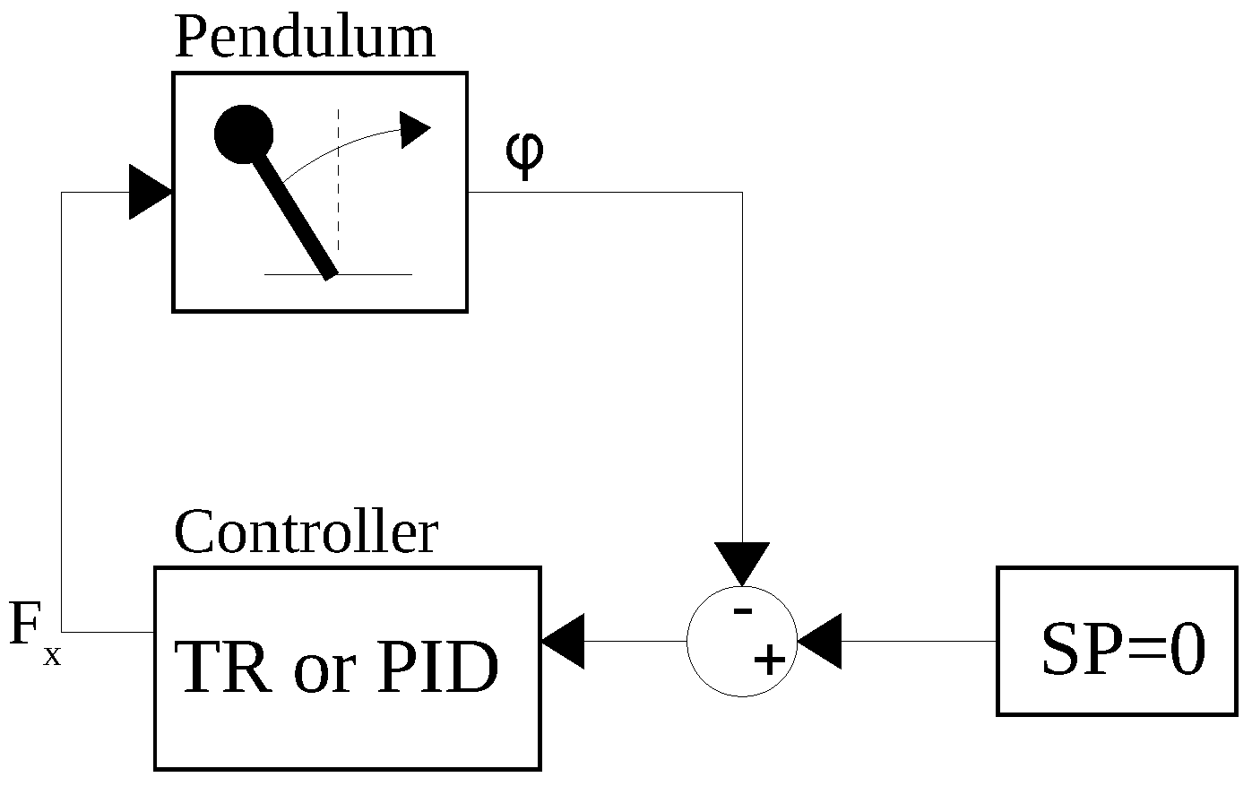
4.1. Simulation Tests of a Control System without Disturbances and Inertial Block

The control system without disturbances and inertial block was connected according to the diagram shown in Figure 2 in order to perform tests. Constant parameters in the system were set in accordance with

Table 1. Constant parameters of the control system.

Description	Symbol	Value	Unit
Mass	m	80	[kg]
Pendulum arm	R	1.2	[m]
Maximum $F_x$	$F_{xmax}$	800	[N]
Minimum $F_x$	$F_{xmin}$	−800	[N]

.

Two control systems were tested: one with a PID controller and the other with a TR controller. It should be noted that in each test, the range of the actuator system was limited in accordance with Table 1. The lack of this limitation greatly facilitated stabilisation, especially when using a PID controller.

Five tests were performed for the TR controller. In each test, the $k_c$ parameter was set to a value of 500. The first three tests showed the influence of the ${\phi }_{min}$ parameter on the quality of control. The initial value of the control system (deviation of the inverted pendulum at the start of the stabilisation process, ${\phi }_0$) was set to ${\phi }_0=1$ ($1radian$ corresponds to 57.3${}^{\circ }$), and the ${\phi }_{min}$ parameter was changed. Tests were performed for ${\phi }_{min}=0$, ${\phi }_{min}=0.05$ (2.86${}^{\circ }$) and ${\phi }_{min}=0.1$ (5.73${}^{\circ }$). In the second part of the TR controller tests, the influence of the initial value on the quality of control was checked. Two additional tests were performed with settings of ${\phi }_0=0.5$ (28.65${}^{\circ }$) and ${\phi }_0=0.2$ (11.46${}^{\circ }$). The value of ${\phi }_{min}$ was set to be constant, and ${\phi }_{min}$ was assumed to be $0.05$. The Author’s experience shows that a value of approximately (3${}^{\circ }$) is an error that may appear in an average inertial measurement system.

In the first stage of testing the PID controller, it was necessary to select the settings. Determining the PID settings was a time-consuming task and did not guarantee the best possible result. In order to select the PID controller settings, the author used tuning tools offered by PID MatLab Simulink and his own experience in this area. To determine these settings, a large number of simulation experiments were carried out. From the obtained results, two sets of PID controller parameters (

Table 2. PID controller settings for the inverted pendulum without disturbances and inertial block (test 1).

P	I	D	N
4109.696	3098.748	1234.512	27.375

and

Table 3. PID controller settings for the inverted pendulum without disturbances and inertial block (test 2).

P	I	D	N
9456.274	1055.274	910.884	12.895

) were selected, and tests with these settings are presented in this study. Tests were conducted for both sets of PID settings, showing the impact of the initial value on the quality of regulation. Tests were performed with settings of ${\phi }_0=1$ (57.3${}^{\circ }$), ${\phi }_0=0.5$ (28.65${}^{\circ }$) and ${\phi }_0=0.2$ (11.46${}^{\circ }$).

The results of the simulation tests of the TR controller are shown in the graphs in Figure 3 and Figure 4, while the results of the simulation tests of the PID controller are shown in the graphs in Figure 5 and Figure 6.

As can be seen from the graphs (Figure 3, Figure 4 and Figure 5), the TR and PID controllers successfully stabilised the inverted pendulum at the equilibrium point. The advantage of the TR controller is the lack of overshoot and the speed of adjustment, although the difference in the rate of adjustment is not large. It should also be noted that the TR controller was very easy to tune, and linear modification of one parameter allowed a satisfactory result to be achieved in a short time. In the case of the PID controller, tuning was very time-consuming. Although the PID controller is a linear controller, the dependence of the control result on the controller settings is highly nonlinear. Correcting the four parameters required a lot of experimentation, and once tuning is complete, there is no certainty that the result achieved is the best possible one.

The graph in Figure 4 shows the influence of the ${\phi }_{min}$ parameter in the system with the TR controller. As can be seen in the graph, the ${\phi }_{min}$ parameter causes the system to stabilise at a level far from the set value. The larger the value of ${\phi }_{min}$, the greater the distance from the set value. As can be seen from the graph in Figure 4, the stabilisation level was below 40% of the ${\phi }_{min}$ value. This means that setting ${\phi }_{min}$ below the measurement accuracy or expected control accuracy should not affect the control accuracy if the measurement error is not constant but oscillates around the correct value.

An interesting result was obtained for ${\phi }_{min}=0$, and despite the threat of dividing by zero, such a phenomenon did not occur. This means that the measured value never reached zero. Thus, a preliminary conclusion can be drawn that the smaller the value of the ${\phi }_{min}$ parameter, the more accurate the control process is. However, in practice, when setting the value of ${\phi }_{min}$, the measurement accuracy and the accuracy of the digital recording of the calculation value should be taken into account, and ${\phi }_{min}$ should be set on this basis.

4.2. Simulation Tests of a Control System with an Inertial Block ($F_{c1}$) of the Actuation System

The control system with an inertial block ($F_{c1}$) of the actuation system was connected according to the diagram shown in Figure 7 in order to perform tests. As before, two control systems were tested: one with a PID controller and the other with a TR controller. In each test, the range of the actuation system was limited in accordance with Table 1. Three tests were performed for the TR controller. In each test, the $k_c$ parameter was set to 500. The tests showed the influence of the inertial block ($F_{c1}$) on the quality of control. As before, during the tests, the value of ${\phi }_{min}=0.05$ was set to be constant, while the initial value of ${\phi }_0$ was changed; in subsequent tests, value of ${\phi }_0=1$ (57.3${}^{\circ }$), ${\phi }_0=0.5$ (28.65${}^{\circ }$) and ${\phi }_0=0.2$ (11.46${}^{\circ }$) were assumed.

For the PID controller, two tests are presented, showing the influence of the inertial block ($F_{c1}$) on the quality of control. The PID controller is a linear controller; therefore, the controller settings selected in previous tests were ineffective. After attaching the inertial block ($F_{c1}$), the system became unstable. It was necessary to reselect the controller settings and carry out a time-consuming procedure. From the obtained results, one set of PID settings was selected (

Table 4. PID controller settings for an inverted pendulum with an inertial block.

P	I	D	N
3934.905	2948.614	1248.676	1473.653

). For the PID, tests were performed, showing the influence of the inertial block ($F_{c1}$) for two initial values. Tests were conducted with settings of ${\phi }_0=0.5$ (28.65${}^{\circ }$) and ${\phi }_0=0.2$ (11.46${}^{\circ }$). For ${\phi }_0=1$ (57.3${}^{\circ }$), no settings were found that would enable the stable operation of the system.

The results of the simulation tests of the TR controller are shown in the graphs in Figure 8, while the results of the simulation tests of the PID controller are shown in the graphs in Figure 9.

As can be seen from the graphs (Figure 8 and Figure 9), the TR and PID controllers successfully stabilised the inverted pendulum at the equilibrium point with settings of ${\phi }_0=0.5$ (28.65${}^{\circ }$) and ${\phi }_0=0.2$ (11.46${}^{\circ }$). However, for ${\phi }_0=1$ (57.3${}^{\circ }$), a stable result was obtained only for the TR controller. The influence of the inertial term is visible in the graphs. Immediately after the start, the control error increases for a while, and only when the force that rectifies the pendulum increases to a value that allows it to counteract the force of gravity do we observe a decrease in the control error. In this respect, the reactions of the two controllers are quite similar. As in the previous test, the advantage of the TR controller is the lack of overshoot and, to a small extent, the speed of reaching the set value. In the PID result graph in Figure 9, a smoother result can be observed when equilibrium is reached. As shown in Section 4.1, the accuracy of the stabilisation of the TR controller depends on the value of the ${\phi }_{min}$ parameter, which, for this test, was set to a value of ${\phi }_{min}=0.05$ (2.86${}^{\circ }$). As in the previous test, the accuracy of achieving the set value for the TR controller was within the range of 40% of the ${\phi }_{min}$ value.

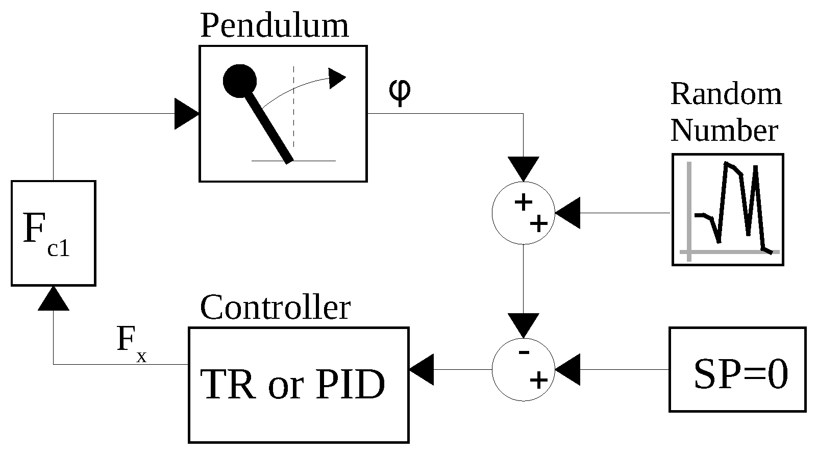
4.3. Simulation Tests of the Control System with an Inertial Block ($F_{c1}$) of the Actuator System and a Disturbance Generator of the Measurement Signal

The control system with an inertial block ($F_{c1}$) of the actuation system and a disturbance generator of the measurement signal was connected according to the diagram shown in Figure 10 in order to perform tests.

The last set of tests was performed similarly to Section 4.2, except that a disturbance was added to the measurement signal. The disturbance was generated using MatLab Simulink’s Random Number block. In the Random Number block, the ’variance’ parameter was set to 0.003, and the time for the generation of disturbing samples was set to 0.01 s. An example of a measurement signal interference is shown in Figure 11. All control system parameters were set as in the control system with an inertial block ($F_{c1}$) of the actuator system, as shown in Section 4.2.

Three tests were performed for the TR controller. In each test, the $k_c$ parameter was set to a value of 500. In the tests, the effect of measurement signal disturbances on the quality of the control was shown. As before, a constant value of ${\phi }_{min}=0.05$ was set during the tests, while the initial ${\phi }_0$ value was changed, taking values of ${\phi }_0=1$ (57.3${}^{\circ }$), ${\phi }_0=0.5$ (28.65${}^{\circ }$) and ${\phi }_0=0.2$ (11.46${}^{\circ }$) in subsequent tests. The test results for the TR controller are shown in Figure 12 and Figure 13.

For the PID, one test is presented to show the effect of measurement signal disturbances on control quality. As the dynamics of the model did not change, all PID controller settings were left the same as in the previous tests (Table 4). However, when interference was introduced into the measurement signal, the system became unstable at settings of ${\phi }_0=0.5$ (28.65${}^{\circ }$) and ${\phi }_0=0.2$ (11.46${}^{\circ }$). A stable response of the system was obtained with a setting of ${\phi }_0=0.1$ (5.73${}^{\circ }$), and for such an initial value (${\phi }_0$), the results are presented in Figure 14 and Figure 15.

As can be seen from the graphs (Figure 12, Figure 13, Figure 14 and Figure 15), the TR and PID controllers successfully stabilised the inverted pendulum at the equilibrium point, but the TR controller performed this task for initial value settings of ${\phi }_0=1$ (57.3${}^{\circ }$), ${\phi }_0=0.5$ (28.65${}^{\circ }$) and ${\phi }_0=0.2$ (11.46${}^{\circ }$), while for the PID controller, a stable result was obtained only after reducing the initial value to ${\phi }_0=0.1$ (5.73${}^{\circ }$). The level of signal adjustment was similar and was in the range of $\pm 0.04radian$. It can also be noticed that despite the disturbances, as in the previous test, the adjustment accuracy for the TR controller was within the range of ${\phi }_{min}$. As in the previous test, the advantage of the TR controller is the lack of overshoot and the speed of readjustment. In this case, disturbances in the measurement signal caused the difference in the time needed to stabilise the system to be clearly visible, in favour of the TR controller. The advantage of the TR controller in this respect is even greater because the TR controller was adjusted from twice the starting value (${\phi }_0$). Figure 12 also shows that the disturbances extended the time to reach the set value of the TR controller itself, especially for the test at ${\phi }_0=1$ (57.3${}^{\circ }$). The adjustment time for this signal almost doubled.

5. Discussion

This study presents a method for the control of an inverted pendulum using the trigonometric function. Inverted pendulum control by the TR controller was compared to the capabilities of the PID controller. Tests of the control system using the PID controller showed the problems associated with using a linear controller for a nonlinear object such as an inverted pendulum. When using a linear controller to control a nonlinear object, we take advantage of the fact that any nonlinearity can be approximated by a linear function around a particular operating point. In practice, this means that a control system operating closer to the operating point is more likely to achieve good stabilisation results using a linear controller. The experiment performed by the author clearly confirmed this phenomenon. The linear PID controller performed best in stabilising the pendulum for small initial values of ${\phi }_0$. The larger the value of ${\phi }_0$ was, the greater the problems with stabilisation of the system. A large initial value led to large tilts of the pendulum, which most often resulted in unstable behaviour of the system. Even in the simplest example, a pendulum without an inertial element, a large overshoot was observed for large values of ${\phi }_0$. In practice, this means that when using a linear controller for a highly nonlinear system, we have to find different controller settings or different linear controller systems for operating points that are far from each other. By monitoring the operating state of the control system, linear control systems can be alternated, or their settings can be changed. This method is commonly used in practice and widely described in the literature. This means that you can use a PID controller and, for example, adjust its settings adaptively [33,34]. Alternatively, at a given operating point, a linear model of the inverted pendulum can be calculated; then, an inverse model can be determined and used for stabilisation [35,36]. The advantage of a solution based on linear modelling is the ability to use a number of mathematical tools that we have for the analysis of linear models. The disadvantage of this approach is the final complexity of the solution and the need for a very time-consuming procedure to tune such a controller for a specific case. Additionally, there is a risk that important elements of the model will be simplified during linearization, and the effect on the real object may be surprising. Similarly, disturbances in the control system can induce states in the working system that go far beyond the linear model. The last set of tests (Section 4.3) showed that the introduction of disturbances into the control system greatly limited the PID controller’s ability to control the inverted pendulum.

Nonlinear solutions such as the TR controller are an alternative to linear systems. The disadvantage of nonlinear systems is often complex mathematical analysis and a lack of consistent knowledge. Often, an uncomplicated nonlinear controller in combination with the control object as a whole constitutes a mathematical model, the analytical solution of which, e.g., in terms of stability, is unattainable. Nonlinear solutions are often unique and difficult to generalise. Hence, in the case of nonlinear systems, simulation tests are one of the basic research methods, as carried out for the TR controller.

On the other hand, it should be remembered that nonlinear controllers open up new possibilities unavailable to linear solutions. In the context of the inverted pendulum, the author was inspired by observing phenomena occurring in nature. The process of stabilising the inverted pendulum can be seen in many animals and humans, e.g., in a quiet standing position. In nature, it can be observed that a newborn animal is able to effectively master learning to maintain balance within a few or a dozen or so seconds, performing only single test movements—and to a large extent, these movements are aimed at improving the efficiency of its muscles rather than learning to balance. The phenomenon we observe in nature is identical to the tuning of an inverted pendulum. Similarly, a human individual is able to maintain balance regardless of a change in his or her centre of gravity or a sudden change in even a previously unknown mass or state of gravity. It should also be noted that the measuring organs at the disposal of humans are not more accurate for many people than, e.g., classic electronic inertial measurement chips of the IMU type. Therefore, it can be expected that there is an inverted pendulum control algorithm that is characterised by simple tuning and stability over a wide range around the operating point. The tests presented in this study showed that the TR controller is a solution that goes in this direction. Tuning the TR controller is simple. There is only one parameter to tune, i.e., $k_c$, and a linear change in this parameter allows for the effective attainment of a stable solution. Furthermore, the range of $k_c$ settings achieving a stable solution is large. As shown in [32], changing the centre of gravity or mass does not destabilise the system. This study shows that the TR controller performs favourably compared with a linear PID controller. The possibilities of the TR controller are much greater than those of the PID controller. The TR controller, unlike the PID controller, effectively stabilises the inverted pendulum in a wide range of ${\phi }_0$ values, regardless of the inertia introduced into the actuator system and the disturbance of the measurement signal. It is worth recalling that in the case of the PID controller, time-consuming retuning was required after the introduction of the inertial module, and after the introduction of disturbances, the capabilities of the PID controller were limited to very small deviations.

6. Conclusions

In summary, it seems that the TR controller developed by the author is an attractive alternative to the applied solutions for stabilising an inverted pendulum around its equilibrium point. The main advantage of this solution is simple tuning of the TR controller, and uncomplicated algorithm structure and good operating efficiency, even at a considerable distance from the operating point. However, it should be noted that the TR controller is a new proposal, and the research space regarding its properties is still open. In a further stage of work, it is possible, for example, to test the effectiveness of the TR algorithm within a wide range of set values of the pendulum inclination angle. The presented research was simplified to a pendulum model in which the righting force is set. In real models, an inverted pendulum is most often used and is placed on a moving cart. If the cart does not move in a circle, it has limited movement space, so in the next stage a test can be performed on such a model. In a system additionally equipped with a trolley, it is necessary to swing the pendulum from the pending position up to the inverted position. When preparing the TR controller to work with an inverted pendulum placed on a cart, it would be necessary to develop an algorithm that combines the possibilities of stabilising the inverted pendulum in the equilibrium position and swinging the pendulum from the pending position. The final test demonstrating the effectiveness of the TR controller should be conducted on a real inverted pendulum model.