Article

Stochastic Subspace Identification-Based Automated Operational Modal Analysis Considering Modal Uncertainty

Structural Engineering Research Institute, Korea Institute of Civil Engineering and Building Technology, 283, Goyangdae-ro, Ilsanseo-gu, Goyang-si 10223, Republic of Korea
*
Author to whom correspondence should be addressed.
Appl. Sci. 2023, 13(22), 12274; https://doi.org/10.3390/app132212274
Submission received: 12 September 2023 / Revised: 20 October 2023 / Accepted: 10 November 2023 / Published: 13 November 2023

Abstract

:

Featured Application

Structural health monitoring.

Abstract

An automated operational modal analysis (AOMA) method that considers the uncertainty in modal parameters is presented and data acquired from actual bridges are used to validate it. The proposed method processes stepwise, from SSI to pre-cleaning, clustering and the removal of outliers. The stochastic subspace identification (SSI) step also calculates the uncertainty of the modal parameters. In this step, the MAC (modal assurance criterion) index and its variability are additionally calculated by exploiting the alteration of the mode shapes. The pre-cleaning stage sorts out the spurious modes by means of the frequency, the coefficient of variation related to the frequency and the damping ratio, as well as the MAC index and its standard deviation. Under the assumption of normal distributions for the frequency and the MAC index, the clustering stage constructs clusters of identical modes with reference to the uncertainty of each mode. The outliers that may be contained in each of these clusters are then removed based upon the frequency, the MAC index and the damping ratio. Values for the parameters that make the proposed method applicable are suggested and are applied unilaterally to three instrumented bridges of different types. The results show that the proposed AOMA method provides accurate mode identification regardless of the bridge type.

1. Introduction

The method of evaluating the health of a structure through measurement generally comprises a process of identifying modes for measurement data, updating the model according to identified modes and evaluating the degree of damage to the structure using the updated model. Depending on the structural health monitoring (SHM) method, the assessment can also be conducted through modal identification, only without any finite element model. For such health evaluation to be available at any time, the whole process should be accomplished without the intervention of the user. The model-updating or damage-assessment processes can be easily automated but this is not the case for modal identification, which points out the necessity of developing a technique allowing the automation of modal identification.
Modal identification is the process of extracting modal parameters, like the natural frequency, damping ratio and mode shape, from measured data. For this process to be executed at any time, operational modal analysis (OMA), which measures only the response of the structure under operation, appears more fitting than experimental modal analysis (EMA), which measures and controls not only the response but also the loading. The usual OMA methods are stochastic subspace identification (SSI) in the time domain [1,2] and frequency domain decomposition (FDD) in the frequency domain [3,4]. However, additional handling of the results provided by these methods is necessary to obtain the actual modes. In SSI, spurious modes must be filtered from the results and the actual modes must be bound in sets of identical modes. In FDD, the actual modes must be extracted from the result curves by peak picking. The whole process without the involvement of an expert and using data measured under operational conditions is called automated operational modal analysis (AOMA).
Brincker et al. [5] proposed a method for identifying the modal domain within predefined limits using a modal coherence function and a modal domain function. However, the method provided different results according to the selection criteria adopted for the peak picking of the results obtained by FDD. A similar method was presented by Magalhães et al. [6] in which sensitivity analysis was applied to the MAC (Modal Assurance Criterion; Allemang [7]) rejection level, but the approach was time-consuming in deciding the values for the diverse parameters and the results based upon the so-decided parameters lacked consistency. Hence, the performance of AOMA based on methods using FDD will depend on the values of the various parameters, including the peak picking criterion.
Vanlanduit et al. [8] employed a series of deterministic and probabilistic criteria as well as a fuzzy clustering approach to obtain the real modes from SSI results. Peeters and De Roeck [9] monitored an actual bridge over the course of one year by applying very simple criteria for selecting only the poles representing more than five modes. Andersen et al. [10] proposed a very fast algorithm to obtain the real poles through the application of graph theory to the stabilization diagram resulting from a multipatch subspace approach, but with slightly degraded reliability. Magalhaes, et al. [11] identified close modes by applying several parameters in a covariance-based SSI (SSI-COV) method, but the approach demanded a large number of calibrations for the computation of the parameters’ values. Here also, the performance of AOMA based on methods using SSI will depend on the criteria chosen for the removal of spurious modes and the removal of outliers. Moreover, it is not guaranteed that criteria that show remarkable performance for a specific bridge will provide equivalent performance when applied to another bridge. A method making it possible to consider this matter is thus necessary.
Reynders et al. [12] analyzed existing research and presented a user-friendly AOMA methodology that consists of three stages: spurious mode removal, clustering and physical mode selection. Cabboi et al. [13] presented a method to automatically analyze the stabilization diagram through checking of the reasonable damping ratio, a modal complexity check and clustering, as well as the introduction of a self-adaptable dynamic threshold to keep track of the modal parameter. As methods for estimating the uncertainty of modal parameters [14,15,16,17,18,19] were developed, methods considering the uncertainty of modal parameters [17,20,21] were presented and methods using machine learning techniques [22,23,24,25] were also studied.
The present study intends to propose a method for extracting real modes from a pool of candidates obtained by SSI-COV. In particular, values of criteria that can be applied consistently to various bridge types are also suggested by exploiting the uncertainty information of individual measured data. Section 2 delivers a summary of SSI-COV that can provide the modal uncertainty. Section 3 introduces the method filtering the real modes and clustering them with respect to the modal uncertainty. Finally, Section 4 validates the effectiveness of the proposed method through its application to actual bridges.

2. Stochastic Subspace Identification with Uncertainty

After a short summary of the existing SSI method and the calculation of the modal uncertainty, this section presents a method for quantifying the uncertainty of the MAC index.

2.1. Stochastic Subspace Identification (SSI)

SSI is a method for extracting modal parameters based on the stochastic state-space model. Owing to its high degree of accuracy compared to other methods, SSI is preferred for OMA. Assuming a white noise external excitation, the following discrete time state-space model of a linear stationary system can be formulated as follows:
x k + 1 = A x k + v k y k = C x k + w k
where x k R n x is the state vector; y k R n y is the output vector; v k R n x and w k R n y are, respectively, the process and output-noise vectors; A R n x × n x is the state matrix of the system; C R n y × n x is the output matrix; and n x and n y are, respectively, the model order and the number of measuring sensors.
A data-driven or covariance-driven technique can be applied to Equation (1). Here, a reference-based covariance-driven technique [26] is adopted for its relatively cheaper analysis burden. First, the block Hankel matrix Y 1 | 2 i 1 R n y 2 i 1 × j is derived from the measured data as follows:
Y 1 | 2 i 1 = y 1 y 2 y j y 2 y 3 y j + 1 y 2 i 1 y 2 i y n d 1 Y 0 | 0 r = y 0 r y 1 r y j 1 r
where Y 0 | 0 r R n y r × j is constructed from the data measured by the reference sensors; n y r is the number of reference sensors; and n d is the number of time steps. If the whole set of data is used, j = n d 2 i , where the time lag i is an integer satisfying the following equation [26]:
i f s 2 f 0
where f s and f 0 are, respectively, the sampling rate and the lowest frequency of interest.
Since the exact output covariance matrix cannot be obtained, unbiased estimates Λ 1 | 2 i 1 r R n y 2 i 1 × n y r are derived from Equation (2) by the following equation.
Λ 1 | 2 i 1 r = 1 j Y 1 | 2 i 1 Y 0 | 0 r T = Λ 1 r Λ 2 r Λ 2 i 1 r
The block Toeplitz matrix L 1 | i r R n y i × n y r i can be obtained from Equation (4).
L 1 | i r = Λ i r Λ i 1 r Λ 1 r Λ i + 1 r Λ i r Λ 2 r Λ 2 i 1 r Λ 2 i 2 r Λ i r = U i Σ i V i T = O i C i r
The singular value decomposition of the block Toeplitz matrix in Equation (5) provides the observability matrix O i R n y i × n x and the controllability matrix C i r R n x × n y r i according to the model order.
O i = U i Σ i 1 / 2 C i r = Σ i 1 / 2 V i T
In Equation (1), A = O i _ O i ¯ is the state matrix, and the output matrix C is the first n y rows of O i . Matrix O i _ is matrix O i of which the last n y rows are removed, matrix O i ¯ is matrix O i of which the first n y rows are removed. Symbol † represents the Moore–Penrose pseudo inverse.
The k -th eigenvalue λ k C and eigenvector φ k C n y can be secured by eigenvalue analysis of the state matrix A .
A φ k = λ k φ k
Subsequently, the k -th modal parameters, like the frequency f k R (Hz), damping ratio ξ k R and mode shape ϕ k C n y , can be calculated.
f k = f s ln λ k 2 π ξ k = R e ln λ k ln λ k ϕ k = C φ k

2.2. Calculation of Uncertainty

The pool of candidate modes obtained by SSI contains real modes but also spurious ones, which should be identified. The real modes have the peculiarity of appearing frequently within a specific frequency range according to the change in the model order. Considering this feature, a stabilization diagram plotting the frequencies of the candidate modes according to the change in the model order is used to sort out the real modes. However, there are no clear criteria about the setting of the specific frequency range nor the number of occurrences that will decide whether a candidate mode within this specific frequency range is a real mode.
Reynders, Pintelon and De Roeck [14] proposed a method for estimating the uncertainty bounds of modal parameters obtained from SSI based upon first-order sensitivity. Later, Döhler and Mevel [15] presented a technique for efficiently calculating these bounds. This technique makes it possible to obtain not only the modal parameters that can usually be derived from SSI but also the uncertainty of each of these parameters. Let σ f k , σ ξ k and σ ϕ k , m be the standard deviation of the natural frequency f k , and let the standard deviation of the damping ratio be ξ k , and the standard deviation of the m -th component ϕ k , m ( m = 1 ,   , n y ) of the mode shape be ϕ k . Since the uncertainty of the modal parameters tends to be small in the case of a real mode, this uncertainty can be exploited as an index discriminating real and spurious modes. In addition, similar modes exhibit similar modal parameters as well as similar uncertainty. Therefore, the uncertainty can also be used as an index for deciding whether two different candidate modes can be assumed to be an identical mode.
Among the uncertainties in modal parameters, the uncertainty in mode shapes can be defined as the uncertainty of MAC. Greś, Döhler and Mevel [18] presented a method for calculating uncertainty of MAC in a strict manner. Another method is to use a Gaussian distribution approximation based on the Central Limit Theorem as shown below. Of these two methods, the former method provides a more accurate uncertainty of MAC.
The distribution of the MAC index of a mode can be obtained from the average and standard deviation of each component of the mode shape. The variability of ϕ k , m is derived from the normal distribution of complex numbers ϕ ~ k , m ~ C N ( ϕ k ,   m ,   σ ϕ k , m 2 ) . The altered mode shape cluster ϕ ~ k of ϕ k can be obtained if this process is applied to all the components. The distribution of the MAC index can be drawn by calculating the MAC indices between the as-obtained ϕ ~ k and ϕ k . This study drew the distribution of the MAC index by finding 1000 altered mode shapes.
Figure 1 compares the cumulative probability distribution (in blue) for the MAC indices of mode shape ϕ k and altered mode shape ϕ ~ k and the cumulative probability distribution (in red) of the normal distribution with average μ M A C k and standard deviation σ M A C k . When the cumulative probability is less than 50%, the sample distribution and the normal distribution are seen to be in relatively good agreement. However, the curves deviate from each other when the cumulative probability becomes higher than 50%. Nevertheless, since the subsequent process uses only that part of the MAC index distribution with cumulative probability lower than 50%, the discrepancy observed above does not constitute a problem. Figure 1a relates to a case with high average and low standard deviation, and Figure 1b to a case with low average and high standard deviation. Both cases show that the MAC index distribution can be approximated by a normal distribution.
The standard deviation σ M A C k can be obtained by equating the MAC value of the sample distribution corresponding to the cumulative probability p and the MAC value of the normal distribution as follows:
q u a n t i l e p = μ M A C k + z p σ M A C k
where q u a n t i l e p is a function determining the MAC value corresponding to the given cumulative probability p for the sample distribution; and z p is the value of the probability function corresponding to the cumulative probability p in the standard normal distribution.
Even if Equation (9) can be applied individually, this study calculates σ M A C k by averaging the values of Equation (9) for p = 0.05 ,   0.10 ,   0.15   a n d     0.20 .
σ M A C k = j q u a n t i l e p j μ M A C k j z p j
The blue and red dots in Figure 1 represent the locations corresponding to p = 0.05 ,   0.10 ,   0.15   a n d   0.20 of the sample distribution and the approximate normal distribution, respectively. The blue and red dots are seen to be practically in coincidence with each other.

3. Automated Operational Modal Analysis Based on Modal Uncertainty

This section presents the method for extracting the real modes from the pool of candidate modes obtained by SSI. The method involves a pre-cleaning process removing the spurious modes from the pool, a clustering process gathering identical modes and a process removing outliers inside the clusters.

3.1. Pre-Cleaning: Removal of Spurious Modes

The pool of candidate modes provided by SSI contains spurious modes that need to be removed. This study cleans these spurious modes by using only basic conditions that real modes must exhibit. Accordingly, the mode cluster resulting from this process will still partially include spurious modes. These remaining spurious modes will be removed in a later process. The basic conditions that should be exhibited by real modes are set as follows: (1) a frequency higher than f s 2 i ( f > f s 2 i ), (2) a coefficient of variation related to the frequency smaller than 0.1 ( C V f = σ f μ f 0.1 ), (3) a damping ratio below 0.1 ( ξ 0.1 ), (4) a MAC index exceeding 0.8 ( μ M A C 0.8 ), and (5) a standard deviation of MAC greater than 0.2 ( σ M A C 0.2 ). Here, σ f , μ f , μ m a c and σ m a c are obtained by the method presented in Section 2.2.
The first condition is driven by Equation (3) from which a computed frequency smaller than f s 2 i indicates a high possibility of having an inaccurate mode. The second condition ( C V f 0.1 ) , which is significantly looser than C V f < 0.015 , which was adopted by Zeng and Hu [21], reduces the risk of removing a real mode. The third condition, that the damping ratio be between 0.1 and 0.2, reduces the risk of removing real modes with low frequencies that are characteristics of civil structures such as bridges. The eventual similarity of the mode shape between two modes is usually decided by looking to see if the MAC value exceeds 80~90% [27]. The fourth condition ( μ M A C 0.8 ) involves the altered mode shape and the average of the MAC values. The fifth condition ( σ M A C 0.2 ) relates to the standard deviation of the MAC values and has a low risk of omitting real modes.
A review of these five conditions reveals that each of them is loose and reduces the risk of removing a real mode. Moreover, there is no need to adjust these conditions for particular measured data since these conditions are lax. However, the application of all these conditions together has been verified to remove practically all the spurious modes (see Section 4).

3.2. Clustering

A check table t i j is constructed to judge whether there are two identical modes in the collection of filtered modes. The frequency and MAC index are compared for two distinct modes.
μ f i μ f j z p σ f j μ M A C j z p σ M A C j M A C μ ϕ i ,   μ ϕ j
If both inequalities of Equation (11) are satisfied, t i j is T r u e or t i j is F a l s e . t i j determines whether the i -th mode is identical to the j -th mode, whereas t j i determines whether the j -th mode is identical to the i -th mode. Note that t i j is not mandatorily equal to t j i . z ( p ) , as the inverse function of the cumulative density function of a standard normal distribution, is a function providing the probabilistic parameter corresponding to the cumulative probability p from the standard normal distribution. In this study, a cumulative probability of 99% is adopted. However, t i j does not show significant change even for a cumulative probability of 95% because, for two modes considered identical, the two modes must exhibit practically similar standard deviations. Consequently, the sensitivity to the cumulative probability p appears to be insignificant. In addition, since this corresponds to a two-sided test for the frequency, and the one-sided test for the MAC index, z p of the one-sided test should be used for the MAC index. However, as the sensitivity is low with regard to z ( p ) , z p of the two-sided test is used. If the decision about whether two modes are identical is made using the standard deviation, the approach can be adapted to modes with different variabilities.
t ¯ i j = t i j     t j i is then constructed from the as-obtained check table, where stands for the conjunction or logical multiplication (AND). t ¯ i j is T r u e only when the two modes are identical, which allows the removal of modes with relatively large variability. The process clustering the identical modes by t ¯ i j is as follows (Figure 2). Cluster C c ( 1 ) of the modes for which the i -th row of t ¯ i j is T r u e is searched. Then, cluster C c ( 2 ) of the modes for which t ¯ i j is T r u e for the row of the searched modes in C c ( 1 ) is extracted. C c is constructed by the combination of C c ( 1 ) and C c ( 2 )   ( C c 1 C c 2 ) . If this process is repeated until the absence of change in C c , the final cluster C c = C c ( 1 ) C c 2 of identical modes can be constructed. If the process is repeated with other modes that are not included in C c , a number n c of clusters C c   ( c = 1 , , n c ) can be formed.

3.3. Removal of Outlier Modes

The clusters of identical modes formed in this way may contain modes with varying characteristics other than frequency and MAC index, so these outlier modes should be removed.
The damping ratio exhibits relatively greater variability than the frequency or the MAC index. If this damping ratio is considered as a condition for the construction of clusters of identical modes, it is likely that the number of clusters would be increased more than necessary. Consequently, the damping ratio is adopted as a criterion for the removal of outliers instead of a criterion for the construction of clusters of identical modes. Check table d i j , related to the modes within one cluster of identical modes is formulated as follows.
μ ξ i μ ξ j z p σ ξ j
The above equation means that the i -th mode related to the j -th mode will exhibit similar damping ratios if satisfied, and that the damping ratio will show different characteristics if not satisfied. A new check table c i j = t i j d i j is constructed by the conjunction (AND) of the check table t i j related to the frequency and MAC index and the check table d i j for the damping ratio.
In the case of a mode with a large standard deviation, a larger number of modes will be recognized as being identical to this mode than there is in reality. Such modes could be spurious modes that have been omitted at the pre-cleaning stage or be modes with other characteristics that should be removed. The number n u m ( c i ) of modes regarded as identical to the i -th mode can be obtained by the number of T r u e columns in the i -th row of matrix c i j . The number n u m c i of modes considered to be identical to the i -th mode can be obtained by the number of T r u e rows in the i -th column of matrix c i j . If we let n u m c i n u m c i apply as the removal criterion and R be the resulting cluster, C ~ c = C c R becomes the cluster of actually identical modes.
For some measured data, modes with the same model order might be present in cluster C ~ c . In such cases, only one mode shall be selected by reckoning that these multiple candidate modes obtained through one execution of SSI correspond to one identical mode. The method adopted to select only one mode is to pick the mode with the smallest standard deviation related to the frequency.
Each of the clusters of identical modes constructed through this process may contain a large or small number of modes. However, since a cluster with an excessively small number of modes might not be a real mode, clusters with a number of modes lower than n m i n ( > 1 ) are excluded. Referring to Ubertini et al. [28], who suggested a range of N 15 ~ N 10 for the number N of SSI analyses, a range of 3~5 is applied.

3.4. Calculation of Mode per Cluster

The representative mode of a cluster of identical modes can be obtained by averaging the modes contained in the cluster or by selecting the peak mode in the normal mixture curve. The following explains the method for the selection of the peak mode in the normal mixture curve. The normal mixture curve can be constructed as follows by using the frequency and the standard deviation of the modes contained in a cluster of identical modes:
y f = k p f ; μ f k , σ f k 2 = k p k f
where p k f is the probability density function of the normal distribution with average μ f k and standard deviation σ f k . The representative mode of the cluster is the peak mode of this normal mixture curve y ( f ) .

3.5. Discussion

A number of parameters are used in the proposed AOMA. However, the parameters adopted in the pre-cleaning stage can be considered as being nearly constant because they were set to prevent the omission of real modes. The other parameters are the cumulative probability p , used for determining whether two modes are identical and n m i n , the minimum number of modes for a cluster of identical modes. Among them, if the cumulative probability p is set to a small value, the cluster will comparatively include only accurate modes. On the other hand, when p is set to a large value, the cluster will include a larger number of modes but p will have a limited effect on the identification of identical modes if p is set within a range of 95~99%. Consequently, the parameter that should be set in reality is the minimum number of modes, but this condition is rarely applied.

4. Case Studies

The effectiveness of the automated modal analysis presented above has been validated. Diverse types of bridge (reinforced concrete rigid-frame bridge, prestressed concrete I-shape girder bridge and prestressed concrete box-shape girder bridge) have been considered to check the applicability of the proposed method. The proposed method adopts various criteria to remove spurious modes or construct clusters of identical modes. If these criteria must be modified according to the structure or the measured data at hand, the method will be unusable. Accordingly, the proposed AOMA was conducted using the values of the criteria listed in Table 1.

4.1. Case Study 1: Prestressed Concrete Box-Shape Girder Bridge

The first bridge chosen for the validation was Hongjaecheon Viaduct, an 8-span continuous prestressed concrete box-shape girder bridge. The bridge has a total length of 380 m (40 + 6 × 50 + 40) and a width of 12.5 m. The sensors were installed in the sixth span, of which the span length is 50 m. The installed sensors are FBG strain sensors, which measured the longitudinal strain at 21 points over 2 h with a sampling frequency of 100 Hz (Figure 3).
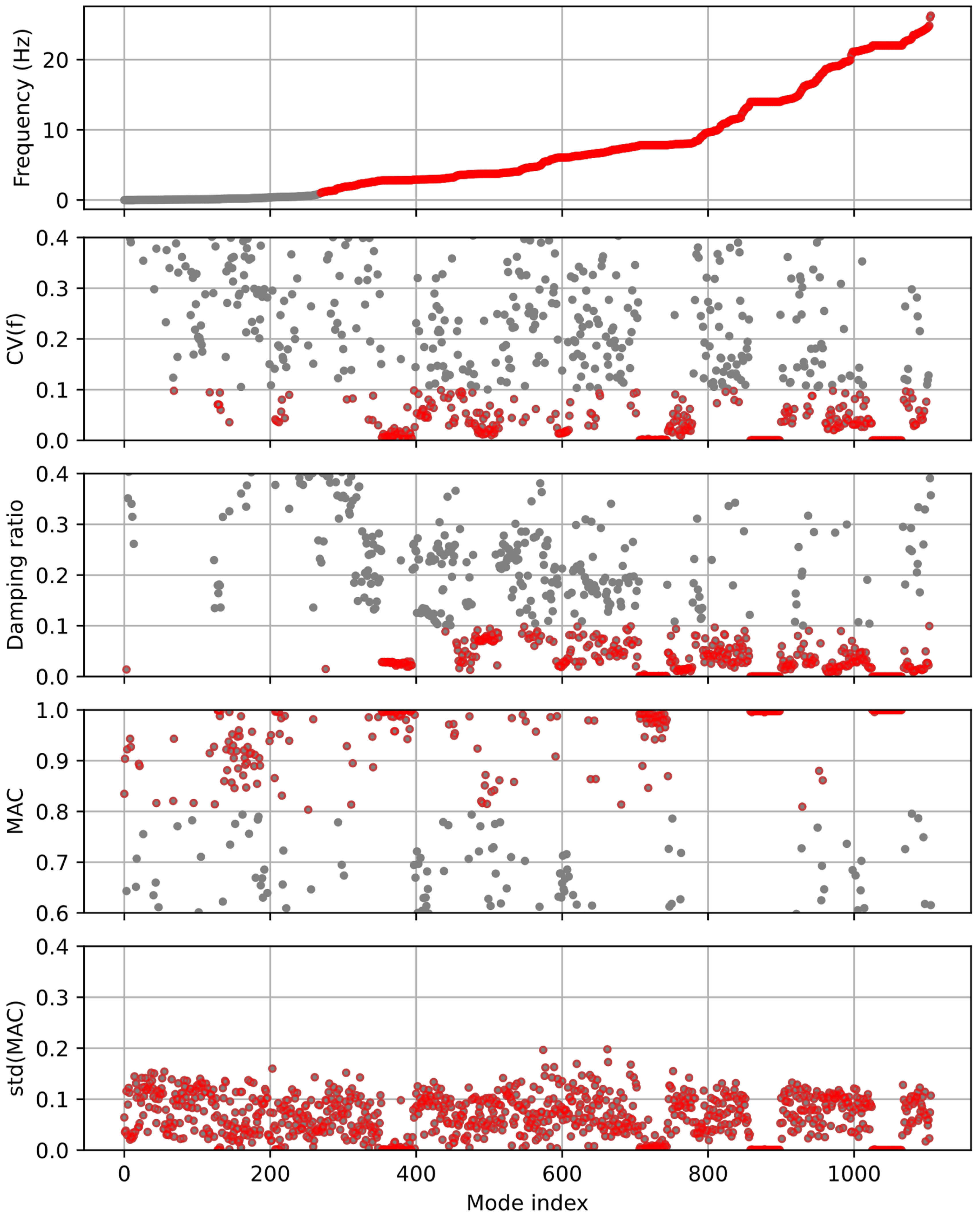
Figure 4 presents the results obtained by applying pre-cleaning criteria to the candidate modes secured by SSI. The horizontal axis in the charts displays the mode index, which corresponds to the serial number attributed to the frequencies of the candidate modes in ascending order. In the charts, the red dots stand for the modes satisfying the pre-cleaning criteria whereas the grey dots represent the modes that do not.
The presence of a series of modes with definite values can be observed around zero for the coefficient of variation for the frequency, the damping ratio and the standard deviation of the MAC index. Modes preserving constant values are also scattered near the MAC index of 1. In addition, the modes exhibiting definite values with regard to specific parameters are also seen to preserve these values for other parameters. These modes maintaining constant values of each parameter can be recognized as real modes. Note that the charts display not only the modes maintaining constant values but also other modes. Consequently, the values chosen for each of the parameters appear to not be so tight as to remove real modes.
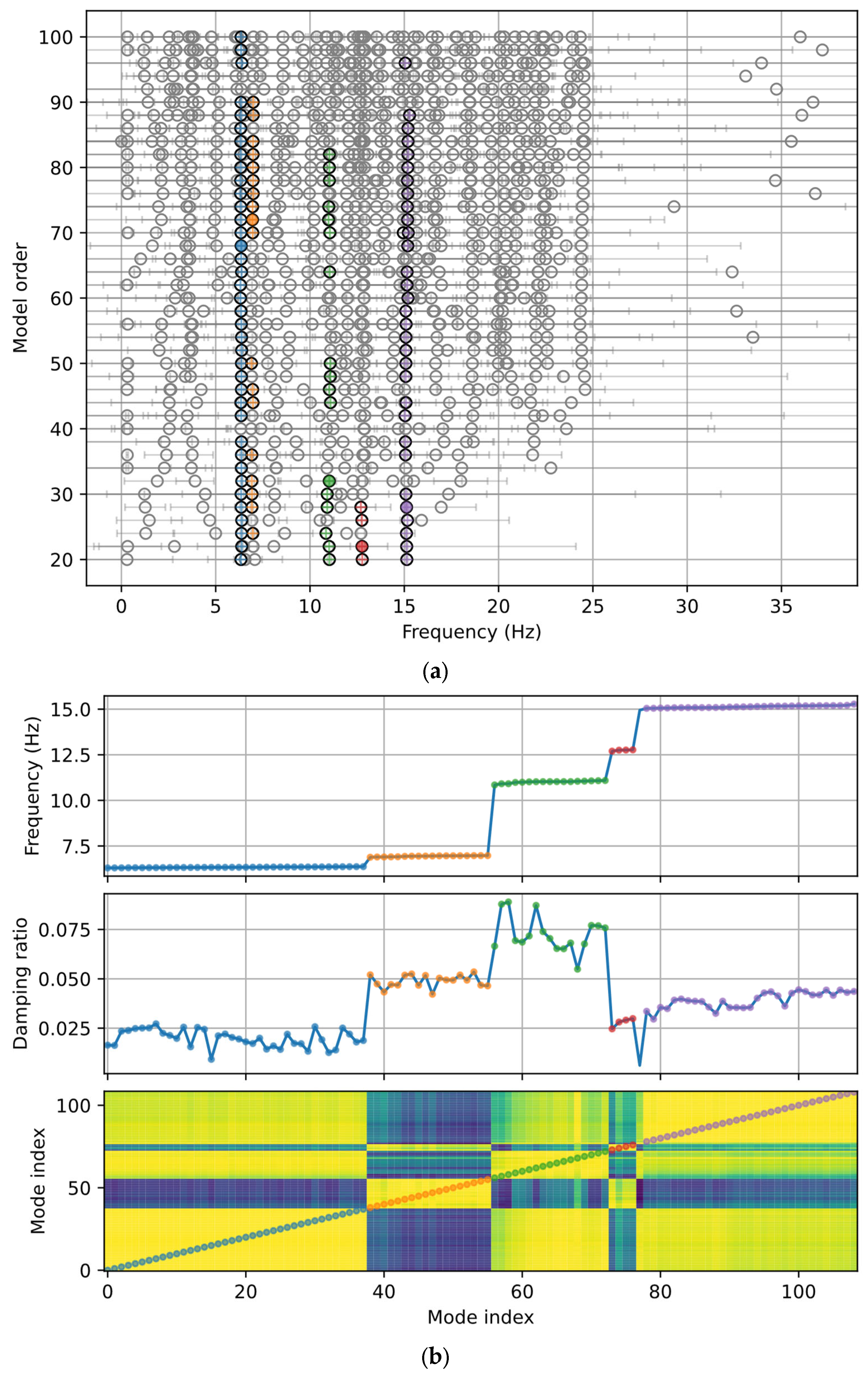
Figure 5a plots the stabilization diagram for the SSI results. The circles in grey represent the modes removed by pre-cleaning, the circles in black are the potential real modes, the colored crosses designate identical modes with the same color, and the solid, colored circles represent the representative modes. Error bars have also been added to indicate the standard deviation of the frequency of each candidate mode. The potential real modes sorted out through the pre-cleaning process are seen to have been accurately selected in the form of poles despite the loose setting of the criteria.
However, it is still difficult to verify that clusters of identical modes have been appropriately constructed by means of the stabilization diagram only. Therefore, Figure 5b plots the modes pre-cleaned with regard to the frequency, damping ratio and MAC index (these diagrams are referred to as Modal Check Diagrams hereafter). Similar to Figure 4, the horizontal axis is the mode index. The dots in the charts distinguish the clusters of identical modes by color. In the charts related to frequency and damping ratio, the modes that can be identified as pertaining to clusters of identical modes are seen to lay in practically horizontal segments. On the other hand, these clusters appear in rectangular blocks in the MAC index chart. The modes exhibiting constant frequency also show a nearly constant damping ratio as well as a rectangular block pattern in the MAC index chart, which indicates that the clusters of identical modes were constructed rationally. This demonstrates that the proposed method makes it possible to filter the spurious modes, construct the clusters of identical modes and remove outliers in a rational manner.

4.2. Case Study 2: Reinforced Concrete Rigid-Frame Bridge

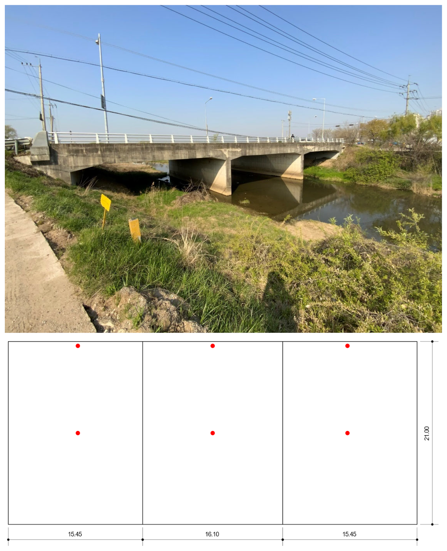
The second bridge selected for the validation was Gajwa Bridge, a 3-span continuous reinforced concrete rigid-frame bridge (Figure 6). The bridge spans a total length of 47 m (15.45 + 16.10 + 15.45) with a width of 21 m. A total of 6 accelerometers were installed in the vertical direction with 1 accelerometer at the center and ends of each span. Measurement was conducted over 4 h at a sampling rate of 100 Hz. This case differs by type of bridge, type of sensor and measured quantities compared to Hongjaecheon Viaduct.
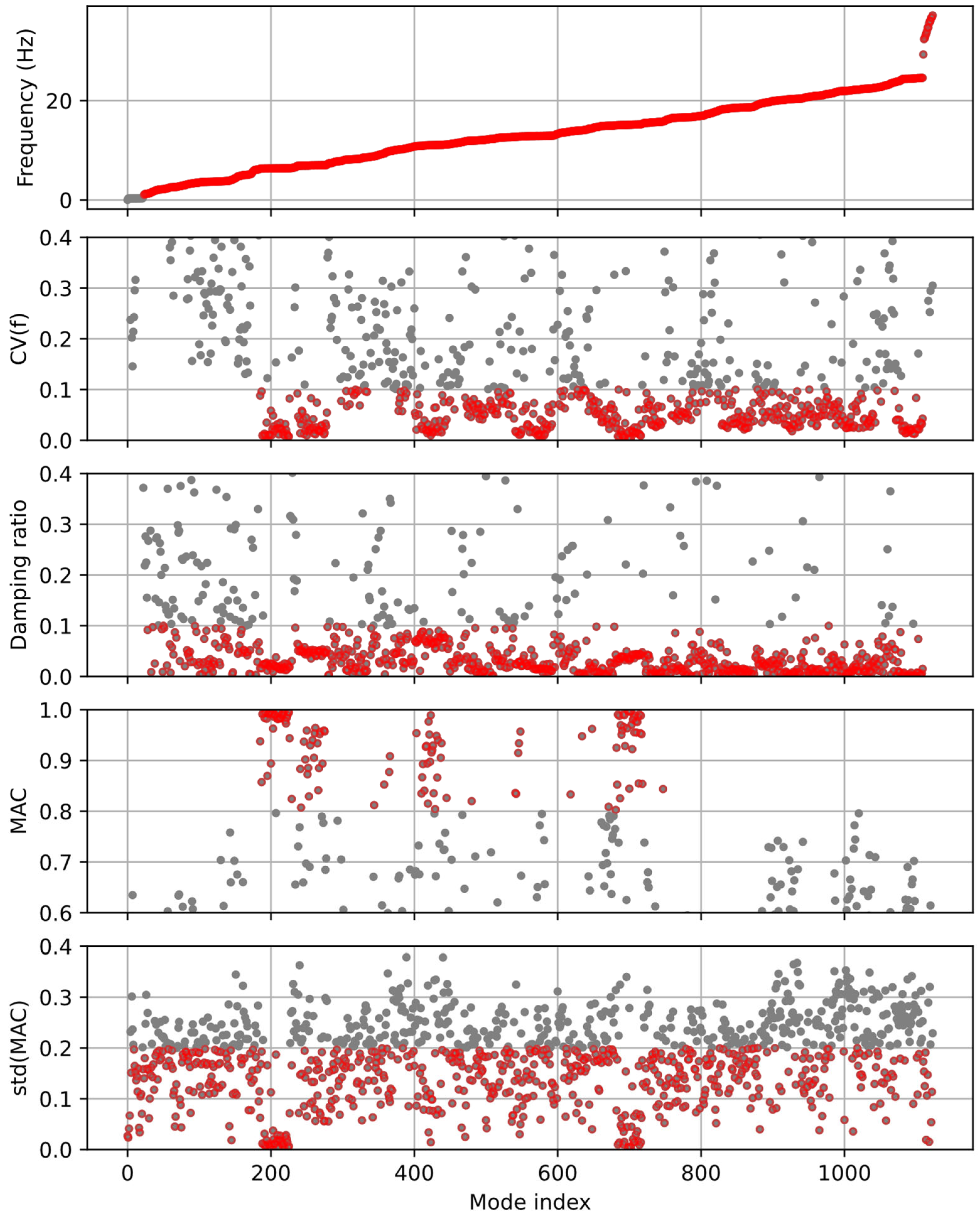
Figure 7 presents the results obtained by applying pre-cleaning criteria to the candidate modes secured by SSI. Sections where the parameters maintain constant values can be distinguished along the frequency arranged in ascending order. It appears that these sections where specific parameters maintain constant values also exhibit constant values for other parameters. The modes contained in these sections can be regarded as real modes. Considering that each individual pre-cleaning criterion does not preclude additional modes, apart from those recognized as being real modes, it can be stated that the pre-cleaning criteria for each separate parameter have been set loosely.
Figure 8 arranges the results provided by the clustering of pre-cleaned modes and the removal of outliers by means of the stabilization diagram and modal check diagram. The pre-cleaned modes indicated in the stabilization diagram appear in the form of poles and show that the pre-cleaning process was appropriately conducted. Here also, the sole stabilization diagram is insufficient to assess the identicality of the mode shapes. Therefore, the modal check diagram plotting the frequency, damping ratio and MAC index of the pre-cleaned modes has been drawn to verify whether the clustering process was appropriately performed. The modes pertaining to clusters of identical modes maintain a constant frequency and also exhibit a high MAC index, from which it is easy to conclude that the constructed clusters are indeed clusters of identical modes.
Even if the damping ratio of the first mode is distributed over a very broad range between 2% and 6%, it is recognized as a cluster of identical modes. This recognition can be done because the assessment was conducted based upon the uncertainty of each mode obtained by SSI without unilaterally setting a range for the identification of clusters of identical modes over the whole set of modes. In other words, if there is large uncertainty about the individual modes obtained by SSI, the range for the recognition of identical modes will also enlarge, whereas a small uncertainty will lead to a narrower range. This fact makes it possible to apply the approach to ranges of clusters of identical modes that can vary according to the bridge type or mode.
Since Gajwa Bridge is a different bridge type than Hongjaecheon Viaduct, it will have different dynamic characteristics. Moreover, the noise is also different because another type of sensor was used and the measured quantities were different. Despite all these differences, the present case study shows that the proposed AOMA performed successfully using the criteria listed in Table 1.

4.3. Case Study 3: Prestressed Concrete I-Shape Girder Bridge

The third bridge for the validation of the proposed method was Hyoja 2 Bridge, which is a single-span bridge with a pre-stressed concrete I-shape girder (Figure 9). The bridge has a length of 30.7 m, a width of 21 m and is skewed by 33°. Two accelerometers were installed in the vertical direction at the center of spans 1 and 3. Measurement was conducted over 4 h at a sampling rate of 100 Hz. This case differs from the other two cases by having a small number of sensors.
Figure 10 plots the results obtained by applying the pre-cleaning criteria to the candidate modes from SSI. This bridge also includes modes other than those presenting a high potential of being real modes while maintaining constant values of the various parameters. Consequently, it can be stated that the pre-cleaning criteria for each individual parameter have been set loosely.
Figure 11 plots the AOMA results by means of the stabilization diagram and modal check diagram. The pre-cleaned modes indicated in the stabilization diagram appear in the form of poles and show that the pre-cleaning process was appropriately conducted. In addition, the natural frequencies of the first and second modes are seen to be fairly close to each other, with values of 6.35 Hz and 6.94 Hz, respectively. It is difficult to verify that these two modes are identical modes by the stabilization diagram only, but an observation of the MAC index chart in the modal check diagram easily shows that these two modes are different with different mode shapes.
In view of the MAC index chart in the modal check diagram, it appears that high MAC indices were computed even for other modes that are not identical modes. This is because of the small number of sensors installed on the bridge. If sensors were installed in sufficient numbers to allow distinguishing of the mode shapes according to the mode, this situation would not occur. However, the proposed method was able to distinguish different modes through the use of not only the MAC index but also the frequency for assessing the identicality of modes.

5. Conclusions

An AOMA method considering the uncertainty of modal parameters was proposed and validated by means of data measured on actual bridges. The proposed method processes stepwise through SSI, the pre-cleaning stage, the clustering stage and the outlier removal stage. The SSI stage calculates the modal parameters together with their uncertainty, and the MAC index and its variability are additionally computed using the mode shape uncertainty. The pre-cleaning stage sorts out the spurious modes by exploiting the frequency, the coefficient of variation related to the frequency, the damping ratio, and the MAC index and its standard deviation. In this stage, the values of the pre-cleaning criteria are set loosely to prevent real modes being removed. Under the assumption of normal distributions for the frequency and the MAC index, the clustering stage constructs clusters of identical modes with reference to the uncertainty of each mode. Finally, outliers that may remain in each cluster of identical modes are removed based upon the frequency, the MAC index, and the damping ratio. Values of the parameters applicable to the proposed method were suggested and applied unilaterally to the AOMA of three bridges of different types. The proposed method and suggested values of the parameters were seen to provide appropriate AOMA for all the considered case studies. The methodology presented here can be applied not only to bridges but also to other structures, in which case verification and parameter calibration would be required.

Author Contributions

Conceptualization, K.C. and J.-R.C.; methodology, K.C.; software, K.C. and J.-R.C.; validation, K.C.; writing—original draft preparation, K.C.; writing—review and editing, K.C. and J.-R.C. All authors have read and agreed to the published version of the manuscript.

Funding

Research for this paper was carried out under the KICT Research Program (project no. 20230073-001, Development of DNA-based smart maintenance platform and application technologies for aging bridges) funded by the Ministry of Science and ICT.

Institutional Review Board Statement

Not applicable.

Informed Consent Statement

Not applicable.

Data Availability Statement

The data presented in this study are available on request from the corresponding author. The data are not publicly available due to Funder’s restriction.

Conflicts of Interest

The authors declare no conflict of interest.

References

  1. Van Overschee, P.; De Moor, B. Subspace Identification for Linear Systems: Theory, Implementation, Applications; Springer: Berlin/Heidelberg, Germany, 1996. [Google Scholar]
  2. Peeters, B.; De Roeck, G. Reference-based stochastic subspace identification for output-only modal analysis. Mech. Syst. Signal Process. 1999, 13, 855–878. [Google Scholar] [CrossRef]
  3. Brincker, R.; Zhang, L.; Andersen, P. Modal identification from ambient responses using frequency domain decomposition. In Proceedings of the 18th International Modal Analysis Conference (IMAC), San Antonio, TX, USA, 7–10 February 2000; pp. 625–630. [Google Scholar]
  4. Brincker, R.; Zhang, L.; Andersen, P. Modal identification of output-only systems using frequency domain decomposition. Smart Mater. Struct. 2001, 10, 441–445. [Google Scholar] [CrossRef]
  5. Brincker, R.; Andersen, P.; Jacobsen, N.-J. Automated frequency domain decomposition for operational modal analysis. In Proceedings of the Conference Proceedings: IMAC-XXIV: A Conference & Exposition on Structural Dynamics, St. Louis, MO, USA, 30 January–2 February 2006. [Google Scholar]
  6. Magalhães, F.; Cunha, Á.; Caetano, E. Dynamic monitoring of a long span arch bridge. Eng. Struct. 2008, 30, 3034–3044. [Google Scholar] [CrossRef]
  7. Allemang, R.J. The modal assurance criterion—Twenty years of use and abuse. Sound Vib. 2003, 37, 14–23. [Google Scholar]
  8. Vanlanduit, S.; Verboven, P.; Guillaume, P.; Schoukens, J. An automatic frequency domain modal parameter estimation algorithm. J. Sound Vib. 2003, 265, 647–661. [Google Scholar] [CrossRef]
  9. Peeters, B.; De Roeck, G. One-year monitoring of the Z24-Bridge: Environmental effects versus damage events. Earthq. Eng. Struct. Dyn. 2001, 30, 149–171. [Google Scholar] [CrossRef]
  10. Andersen, P.; Brincker, R.; Goursat, M.; Mevel, L. Automated modal parameter estimation for operational modal analysis of large systems. In Proceedings of the 2nd International Operational Modal Analysis Conference, Copenhagen, Denmark, 30 April–2 May 2007; pp. 299–308. [Google Scholar]
  11. Magalhaes, F.; Cunha, A.; Caetano, E. Online automatic identification of the modal parameters of a long span arch bridge. Mech. Syst. Signal Process. 2009, 23, 316–329. [Google Scholar] [CrossRef]
  12. Reynders, E.; Houbrechts, J.; De Roeck, G. Fully automated (operational) modal analysis. Mech. Syst. Signal Process. 2012, 29, 228–250. [Google Scholar] [CrossRef]
  13. Cabboi, A.; Magalhaes, F.; Gentile, C.; Cunha, A. Automated modal identification and tracking: Application to an iron arch bridge. Struct. Control Health Monit. 2017, 24, e1854. [Google Scholar] [CrossRef]
  14. Reynders, E.; Pintelon, R.; De Roeck, G. Uncertainty bounds on modal parameters obtained from stochastic subspace identification. Mech. Syst. Signal Process. 2008, 22, 948–969. [Google Scholar] [CrossRef]
  15. Döhler, M.; Mevel, L. Efficient multi-order uncertainty computation for stochastic subspace identification. Mech. Syst. Signal Process. 2013, 38, 346–366. [Google Scholar] [CrossRef]
  16. Reynders, E.; Maes, K.; Lombaert, G.; De Roeck, G. Uncertainty quantification in operational modal analysis with stochastic subspace identification: Validation and applications. Mech. Syst. Signal Process. 2016, 66–67, 13–30. [Google Scholar] [CrossRef]
  17. Pereira, S.; Reynders, E.; Magalhaes, F.; Cunha, A.; Gomes, J.P. The role of modal parameters uncertainty estimation in automated modal identification, modal tracking and data normalization. Eng. Struct. 2020, 224, 111208. [Google Scholar] [CrossRef]
  18. Greś, S.; Döhler, M.; Mevel, L. Uncertainty quantification of the modal assurance criterion in operational modal analysis. Mech. Syst. Signal Process. 2021, 152, 107457. [Google Scholar] [CrossRef]
  19. Greś, S.; Riva, R.; Süleyman, C.Y.; Andersen, P.; Łuczak, M.M. Uncertainty quantification of modal parameter estimates obtained from subspace identification: An experimental validation on a laboratory test of a large-scale wind turbine blade. Eng. Struct. 2022, 256, 114001. [Google Scholar] [CrossRef]
  20. He, Y.; Yang, J.P.; Li, Y.F. A three-stage automated modal identification framework for bridge parameters based on frequency uncertainty and density clustering. Eng. Struct. 2022, 255, 113891. [Google Scholar] [CrossRef]
  21. Zeng, J.C.; Hu, Z. Automated operational modal analysis using variational Gaussian mixture model. Eng. Struct. 2022, 273, 115139. [Google Scholar] [CrossRef]
  22. Favarelli, E.; Giorgetti, A. Machine Learning for Automatic Processing of Modal Analysis in Damage Detection of Bridges. IEEE Trans. Instrum. Meas. 2021, 70, 2504013. [Google Scholar] [CrossRef]
  23. Mugnaini, V.; Fragonara, L.Z.; Civera, M. A machine learning approach for automatic operational modal analysis. Mech. Syst. Signal Process. 2022, 170, 108813. [Google Scholar] [CrossRef]
  24. Civera, M.; Mugnaini, V.; Fragonara, L.Z. Machine learning-based automatic operational modal analysis: A structural health monitoring application to masonry arch bridges. Struct. Control Health Monit. 2022, 29, e3028. [Google Scholar] [CrossRef]
  25. Cheema, P.; Alamdari, M.M.; Vio, G.A.; Zhang, F.L.; Kim, C.W. Infinite mixture models for operational modal analysis: An automated and principled approach. J. Sound Vib. 2021, 491, 115757. [Google Scholar] [CrossRef]
  26. Reynders, E.; Roeck, G.D. Reference-based combined deterministic–stochastic subspace identification for experimental and operational modal analysis. Mech. Syst. Signal Process. 2008, 22, 617–637. [Google Scholar] [CrossRef]
  27. Rainieri, C.; Fabbrocino, G.; Cosenza, E. Near real-time tracking of dynamic properties for standalone structural health monitoring systems. Mech. Syst. Signal Process. 2011, 25, 3010–3026. [Google Scholar] [CrossRef]
  28. Ubertini, F.; Gentile, C.; Materazzi, A.L. Automated modal identification in operational conditions and its application to bridges. Eng. Struct. 2013, 46, 264–278. [Google Scholar] [CrossRef]
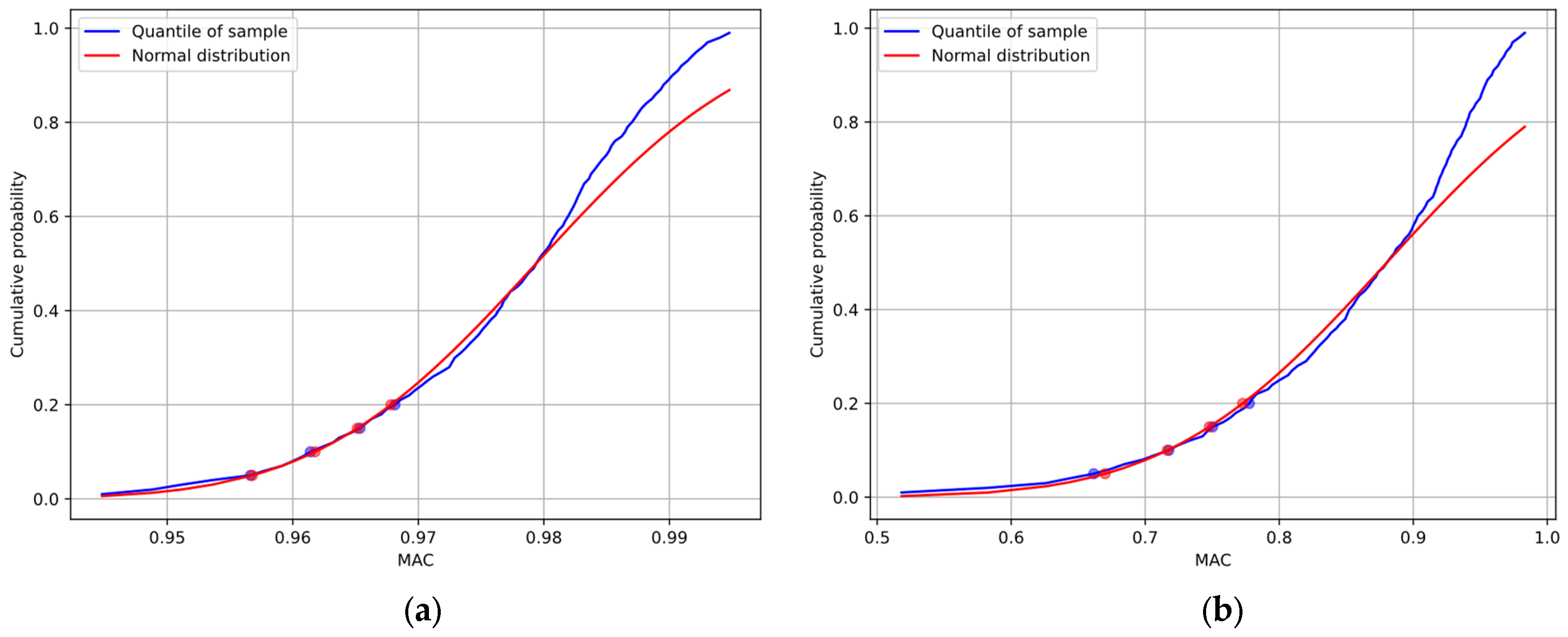
Figure 1. Comparison of cumulative probability distributions of sample MAC index distribution and normal distribution. (a) Case with high average and low standard deviation; (b) case with low average and high standard deviation.
Applsci 13 12274 g001
Figure 2. Process of finding a cluster of identical modes by t ¯ i j (blank cell indicates F a l s e ).
Applsci 13 12274 g002
Figure 3. Shape and sensor layout of Hongjaecheon Viaduct.
Applsci 13 12274 g003
Figure 4. Pre-cleaning results for Hongjaecheon Viaduct (The red dots indicate the modes satisfying the pre-cleaning criteria).
Applsci 13 12274 g004
Figure 5. Hongjaecheon Viaduct: (a) stabilization diagram; (b) modal check diagram.
Applsci 13 12274 g005
Figure 6. Shape and sensor layout of Gajwa Bridge (The red dots indicate sensor locations).
Applsci 13 12274 g006
Figure 7. Pre-cleaning results for Gajwa Bridge (The red dots indicate the modes satisfying the pre-cleaning criteria).
Applsci 13 12274 g007
Figure 8. Gajwa Bridge: (a) stabilization diagram; (b) modal check diagram.
Applsci 13 12274 g008
Figure 9. Shape and sensor layout of Hyoja 2 Bridge (The red dots indicate sensor locations).
Applsci 13 12274 g009
Figure 10. Pre-cleaning results for Hyoja 2 Bridge (The red dots indicate the modes satisfying the pre-cleaning criteria).
Applsci 13 12274 g010
Figure 11. Hyoja 2 Bridge: (a) stabilization diagram; (b) modal check diagram.
Applsci 13 12274 g011
Table 1. Criteria for automated modal analysis.
Pre-Cleaning CriteriaCriteria for Clustering and
Removal of Outliers
f f s 2 i
C V f = σ f μ f 0.1
ξ 0.1
μ M A C 0.8
σ M A C 0.2
p = 0.99
n m i n = 3
Disclaimer/Publisher’s Note: The statements, opinions and data contained in all publications are solely those of the individual author(s) and contributor(s) and not of MDPI and/or the editor(s). MDPI and/or the editor(s) disclaim responsibility for any injury to people or property resulting from any ideas, methods, instructions or products referred to in the content.