

Dynamic Mechanical Properties of Heat-Treated Shale under Different Temperatures

Abstract
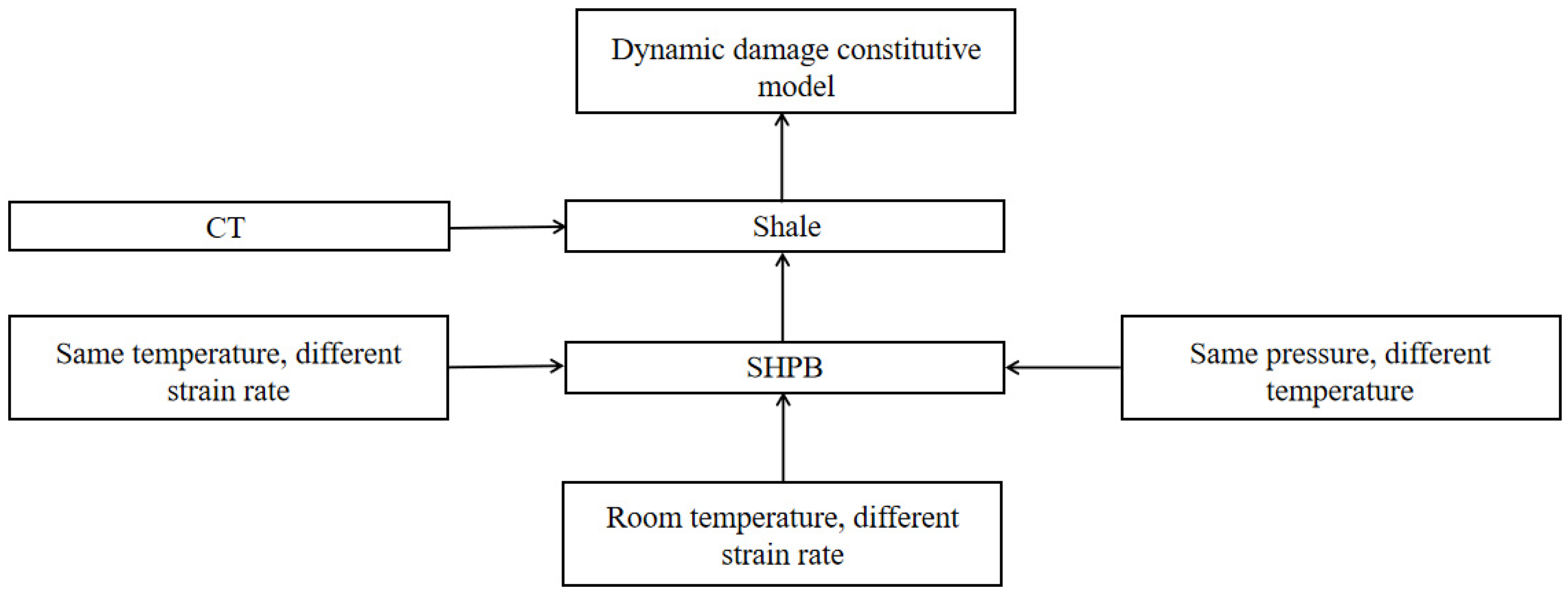
:1. Introduction
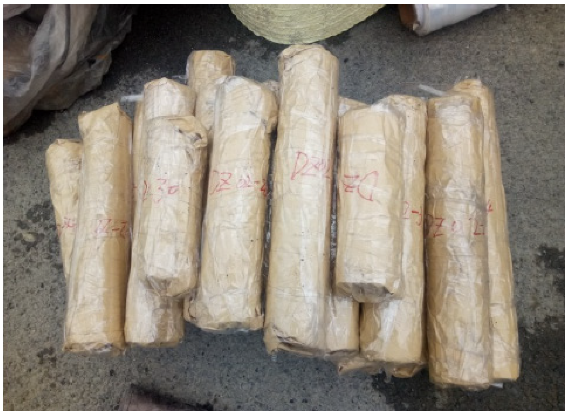
2. Preparation of Shale Specimen
2.1. Sampling and Processing
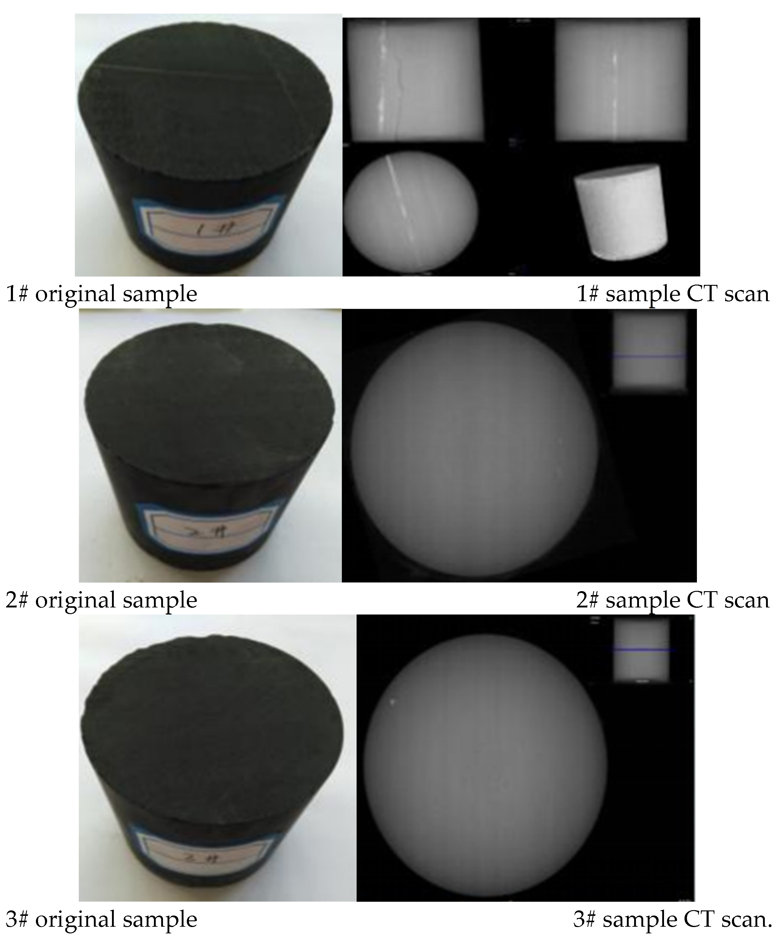
2.2. Shale CT Scanning and Material Composition
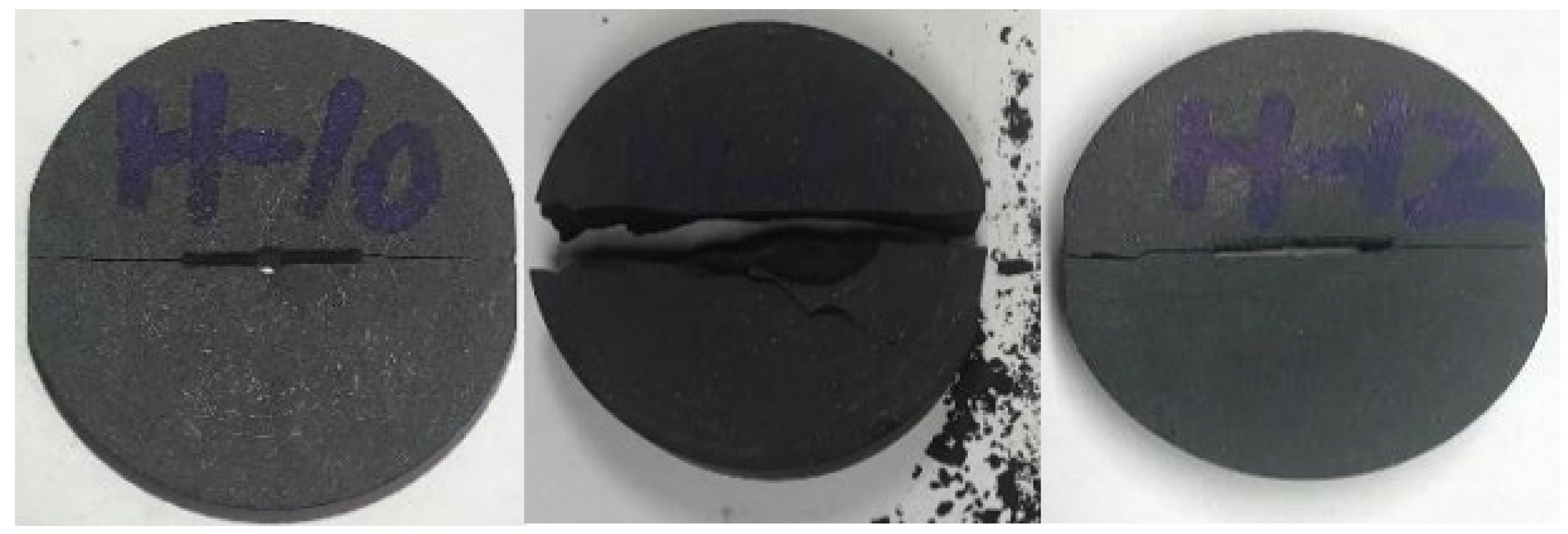
3. Splitting and Stretching Test
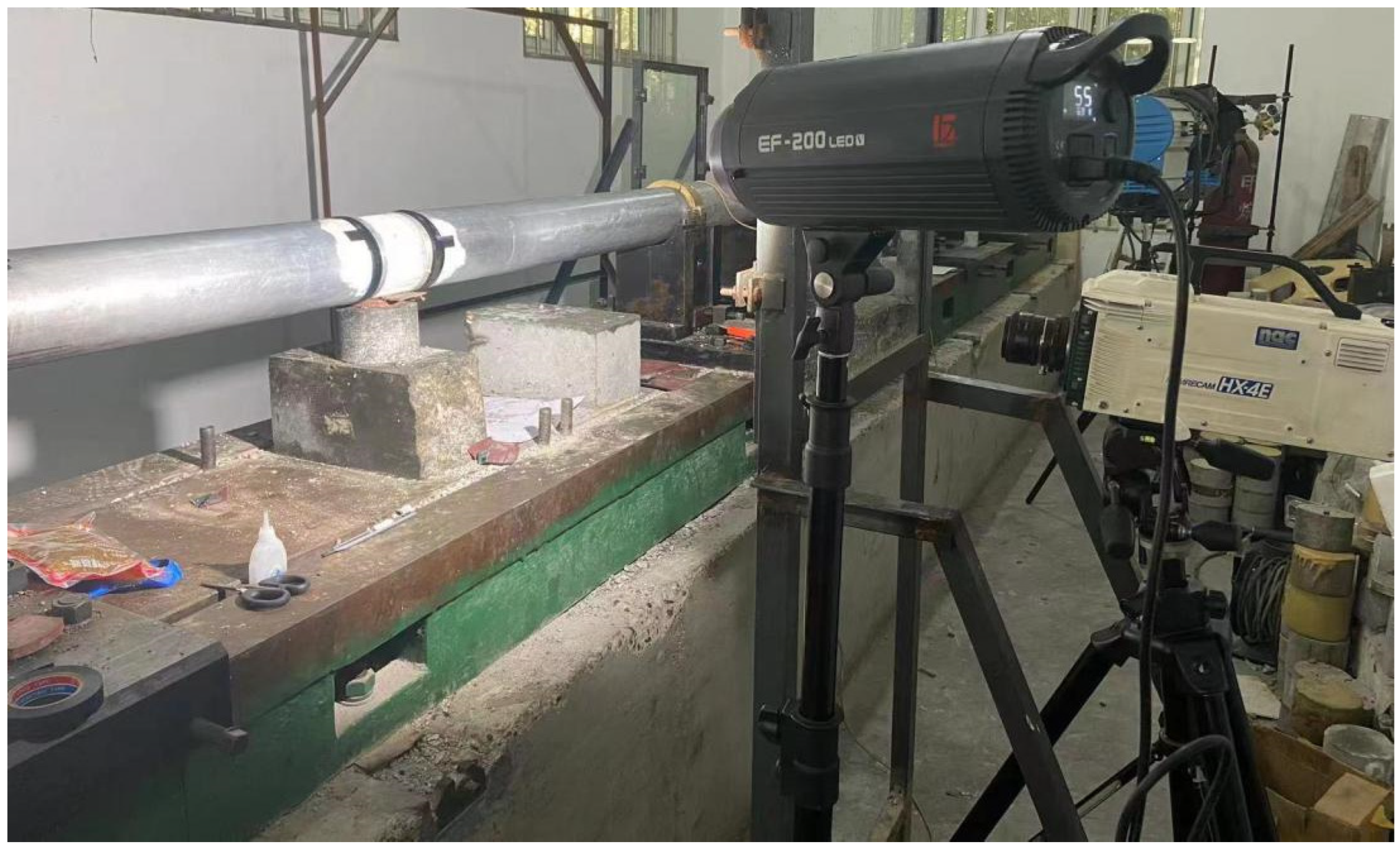
4. Shale SHPB Experiment
5. Analysis of the Experimental Results
5.1. Stress Balance Check and Typical Failure Modes of Shale Specimens
5.2. Stress–Strain Curve of Shale Material at Room Temperature
5.3. Dynamic Compressive Strength Analysis of Shale
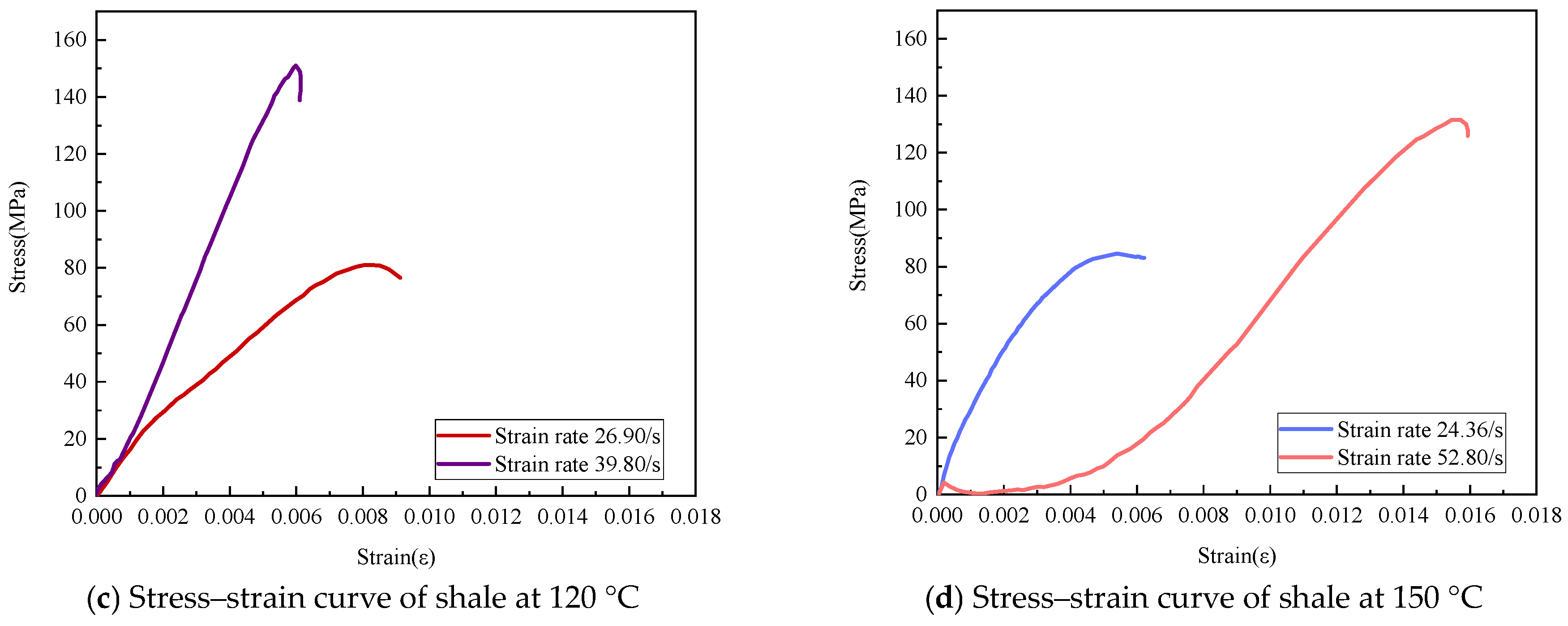
5.4. Analysis of Shale under the Same Temperature and Different Strain Rates
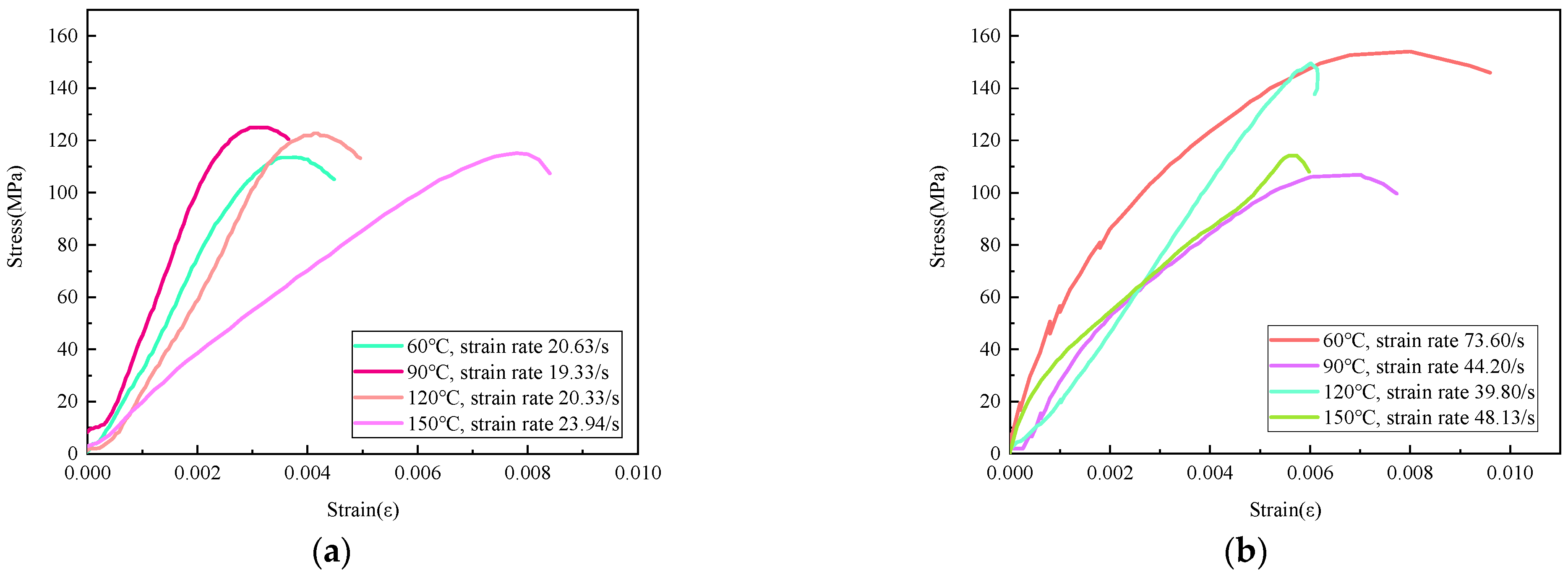
5.5. Analysis of Shale under the Same Pressure and Different Temperatures
6. Dynamic Damage Constitutive Model
6.1. Definition of Damage Variable
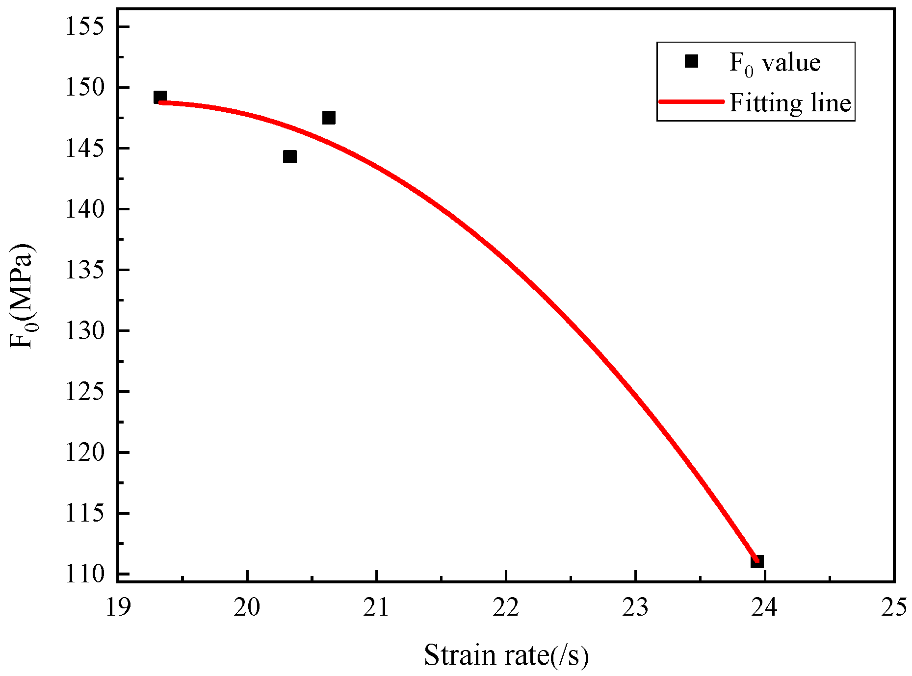
6.2. Micro-Body Strength
6.3. Establishment and Modification of the Constitutive Model
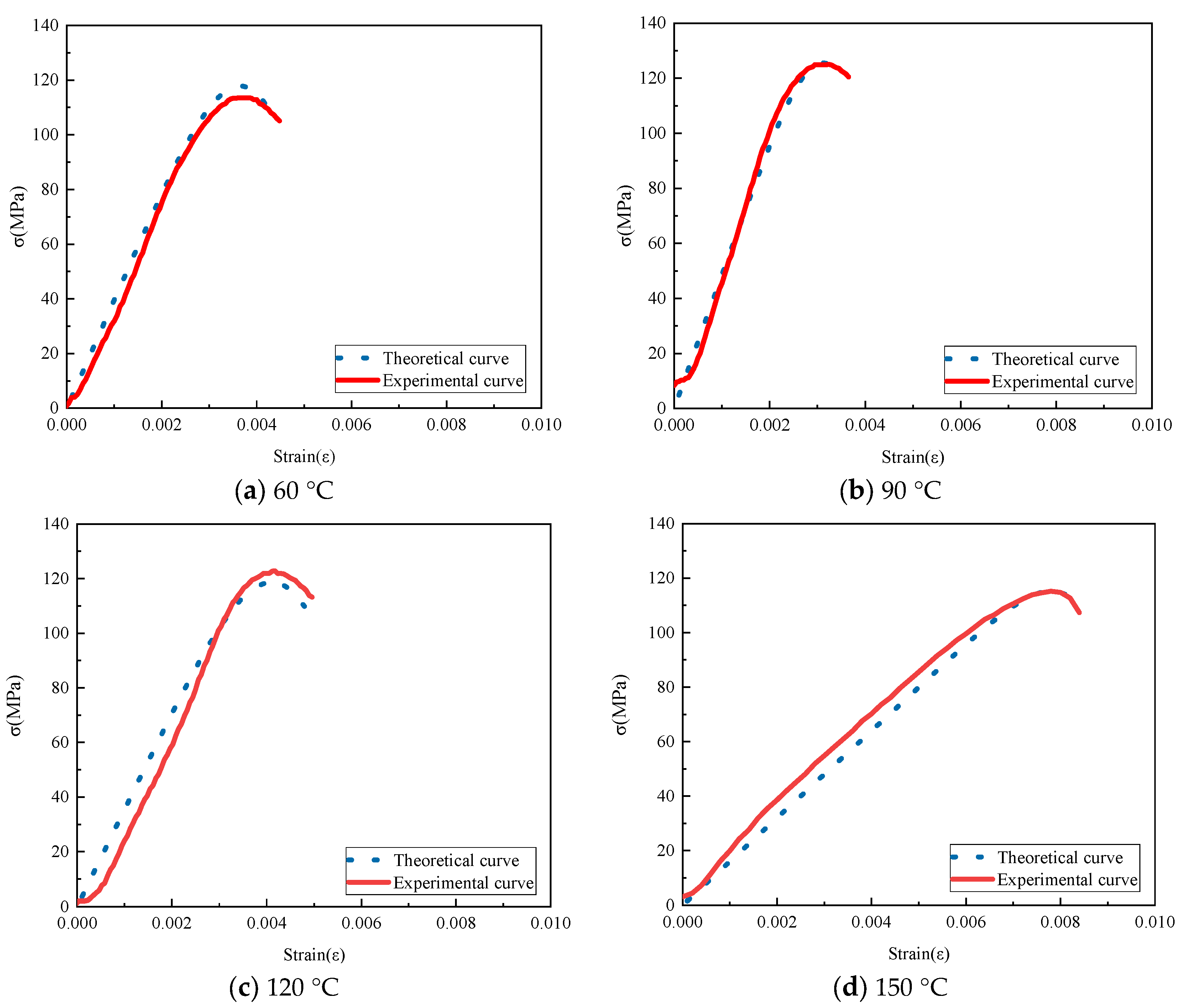
6.4. Verification of the Constitutive Model
7. Conclusions
Author Contributions
Funding
Institutional Review Board Statement
Informed Consent Statement
Data Availability Statement
Conflicts of Interest
References
- Li, W.K. Application of high-energy gas fracturing technology in oil and gas resource development. J. Earth Sci. Environ. 2000, 22, 60–62. (In Chinese) [Google Scholar]
- Zhang, D.Y.; Zhang, X.Y. Research and application of high energy gas fracturing technology. Oil Drill. Prod. Technol. 1997, 19, 17–23. (In Chinese) [Google Scholar]
- Wang, H. Study on Evaluation of Compressibility of High Energy Gas Fracturing for Horizontal Wells in Shale Gas Reservoirs; Xi’an Shiyou University: Xi’an, China, 2016. [Google Scholar]
- Horsrud, P.; Sønstebø, E.; Bøe, R. Mechanical and petrophysical properties of North Sea shales. Int. J. Rock Mech. Min. Sci. 1998, 35, 1009–1020. [Google Scholar] [CrossRef]
- Hsu, S.-C.; Nelson, P.P. Characterization of Eagle Ford Shale. Eng. Geol. 2002, 67, 169–183. [Google Scholar] [CrossRef]
- Sarout, J.; Molez, L.; Guéguen, Y.; Hoteit, N. Shale dynamic properties and anisotropy under triaxial loading: Experimental and theoretical investigations. Phys. Chem. Earth Parts A/B/C 2007, 32, 896–906. [Google Scholar] [CrossRef]
- Niandou, H.; Shao, J.; Henry, J.; Fourmaintraux, D. Laboratory investigation of the mechanical behaviour of Tournemire shale. Int. J. Rock Mech. Min. Sci. 1997, 34, 3–16. [Google Scholar] [CrossRef]
- Kuila, U.; Dewhurst, D.; Siggins, A. Raven Stress anisotropy and velocity anisotropy in low porosity shale. Tectonophysics 2011, 503, 34–44. [Google Scholar] [CrossRef]
- Luo, N.; Fan, X.; Cao, X.; Zhai, C.; Han, T. Dynamic mechanical properties and constitutive model of shale with different bedding under triaxial impact test. J. Pet. Sci. Eng. 2022, 216, 110758. [Google Scholar] [CrossRef]
- Huang, L.; Guo, Y.; Li, X. Mechanical response to dynamic compressive load applied to shale after thermal treatment. J. Nat. Gas Sci. Eng. 2022, 102, 104565. [Google Scholar] [CrossRef]
- Dong, D.Z.; Zou, C.N.; Yang, H.; Wang, Y.M.; Li, X.J.; Chen, G.S.; Wang, S.Q.; Lv, Z.G.; Huang, Y.B. Progress and prospect of shale gas exploration and development in China. Acta Pet. Sin. 2012, 33, 107–114. (In Chinese) [Google Scholar]
- Heng, S.; Yang, C.H.; Zhang, B.P.; Guo, Y.T.; Wang, L.; Wei, Y.L. Experimental study on anisotropy characteristics of shale. Rock Soil Mech. 2015, 36, 609–616. (In Chinese) [Google Scholar]
- Peng, G.Z. Relationship between structural plane orientation and mechanical properties of shale rock under uniaxial compressive stress. Chin. J. Geotech. Eng. 1983, 2, 101–109. (In Chinese) [Google Scholar]
- Liu, G.J.; Xian, X.F.; Zhou, J.P.; Zhang, L.; Liu, Q.L.; Zhang, S.W. Experimental study on deformation characteristics of shale under load and influence of mineral components on rock brittleness. J. China Coal Soc. 2016, 41, 369–375. (In Chinese) [Google Scholar]
- Kang, Z.Q. Simulation Study on Pyrolysis Characteristics of Oil Shale and in-Situ Thermal Injection for Oil and Gas Production; Taiyuan University of Technology: Taiyuan, China, 2008. (In Chinese) [Google Scholar]
- Deng, J.X.; Tang, Z.Y.; Li, Y.; Xie, J.; Liu, H.L.; Guo, W. Influence of diagenetic process on seismic petrophysical characteristics of shale in Wufeng-Longmaxi Formation. Chin. J. Geophys. 2018, 61, 659–672. (In Chinese) [Google Scholar]
- Wang, Y.; Xu, J.; Mei, C.G.; Ou, B.; Li, L. Study on physicochemical and mechanical properties of hard brittle shale with fractures. J. Oil Gas Technol. 2011, 33, 104–108+9. (In Chinese) [Google Scholar]
- Liu, J.X.; Liu, W.; Yang, C.H.; Huo, L. Experimental study on mechanical properties of mud shale under different strain rates. Rock Soil Mech. 2014, 35, 3093–3100. (In Chinese) [Google Scholar]
- Liu, J.X.; Zhang, K.; Liu, W.; Shi, X.L. Experimental study on deformation and failure characteristics of shale under different confining pressures and strain rates. Rock Soil Mech. 2017, 38, 43–52. (In Chinese) [Google Scholar]
- Zhang, H.J. Shale Dynamic Constitutive Relationship and Its Application; Southwest Petroleum University: Sichuan, China, 2014. (In Chinese) [Google Scholar]
- Yang, G.L.; Bi, J.J.; Zhang, Z.F.; Li, X.G.; Liu, J.; Hong, P.X. Effect of bedding angle under passive confining pressure on dynamic strength and energy dissipation of shale. J. Min. Sci. Technol. 2021, 6, 188–195. (In Chinese) [Google Scholar]
- Abbas, H.A.; Mohamed, Z.; Kudus, S.A. Deformation behaviour, crack initiation and crack damage of weathered composite sandstone-shale by using the ultrasonic wave and the acoustic emission under uniaxial compressive stress. Int. J. Rock Mech. Min. Sci. 2023, 170, 105497. [Google Scholar] [CrossRef]
- Fan, L.; Yi, X.; Ma, G. Numerical manifold method (NMM) simulation of stress wave propagation through fractured rock mass. Int. J. Appl. Mech. 2013, 5, 1350022. [Google Scholar] [CrossRef]
- Zhou, X.; Fan, L.; Wu, Z. Effects of microfracture on wave propagation through rock mass. Int. J. Geomech. 2017, 17, 04017072. [Google Scholar] [CrossRef]
- Fan, L.; Gao, J.; Du, X.; Wu, Z. Spatial gradient distributions of thermal shock-induced damage to granite. J. Rock Mech. Geotech. Eng. 2020, 12, 917–926. [Google Scholar] [CrossRef]
- Fan, L.F.; Wu, Z.J.; Wan, Z.; Gao, J.W. Experimental investigation of thermal effects on dynamic behavior of granite. Appl. Therm. Eng. 2017, 125, 94–103. [Google Scholar] [CrossRef]
- Baldin, M.T.; Salamuni, E.; Lagoeiro, L.E.; Sanches, E. High-temperature deformation processes in migmatites from the Atuba Complex, southern Ribeira Belt: Constrains from microstructures and EBSD analyses. J. South Am. Earth Sci. 2022, 116, 103863. [Google Scholar] [CrossRef]
- SAnsari, S.A.; Kazim, M.; Khaliq, M.A.; Ratlamwala, T.A.H. Thermal analysis of multigeneration system using geothermal energy as its main power source. Int. J. Hydrog. Energy 2020, 46, 4724–4738. [Google Scholar] [CrossRef]
- Zheng, Y.; Jia, C.; Zhang, S.; Shi, C. Experimental and constitutive modeling of the anisotropic mechanical properties of shale subjected to thermal treatment. Geomech. Energy Environ. 2023, 35, 100485. [Google Scholar] [CrossRef]
- Zhang, K. Effect of Anisotropy on Mechanical Properties and Strain Rate Effect of Shale; Southwest University of Science and Technology: Mianyang, China, 2017. (In Chinese) [Google Scholar]
- Liao, J.S. Study on Mechanical Properties of Shale under Uniaxial Lateral Confinement; Southwest University of Science and Technology: Mianyang, China, 2018. (In Chinese) [Google Scholar]
- Kolsky, H. An Investigation of the Mechanical Properties of Materials at Very High Rates of Strain. Proc. Phys. Soc. Sect. B 1949, 62, 676–700. [Google Scholar] [CrossRef]
- ANSI/B0019QEADC; Metals Handbook—Ninth Edition. American Society for Metals: Detroit, MI, USA, 1985.
- Chen, W.; Ravichandran, G. Dynamic compressive failure of a glass ceramic under lateral confinement. J. Mech. Phys. Solids 1997, 45, 1303–1328. [Google Scholar] [CrossRef]
- Jia, B. Study on Static and Dynamic Characteristics of Concrete at High Temperature; Chongqing University: Chongqing, China, 2011. (In Chinese) [Google Scholar]
- Lv, T.H. Study on Mechanical Behavior of Concrete and Reinforced Concrete under Impact Compression Based on SHPB; University of Science and Technology of China: Hefei, China, 2018. (In Chinese) [Google Scholar]
- Li, Q.M.; Meng, H. About the dynamic strength enhancement of concrete-like materials in a split Hopkinson pressure bar test. Int. J. Solids Struct. 2003, 40, 343–360. [Google Scholar] [CrossRef]
- Tedesco, J.W.; Ross, C.A.; McGill, P.B.; O’Neil, B.P. Numerical analysis of high strain rate concrete direct tension tests. Comput. Struct. 1991, 40, 313–327. [Google Scholar] [CrossRef]
- Wu, H.; Zhang, Q.; Huang, F.; Jin, Q. Experimental and numerical investigation on the dynamic tensile strength of concrete. Int. J. Impact Eng. 2005, 32, 605–617. [Google Scholar] [CrossRef]
- Krajcinovic, D.; Rinaldi, A. Statistical Damage Mechanics—Part I: Theory. J. Appl. Mech. 2005, 72, 76–85. [Google Scholar] [CrossRef]
- Xu, X.; Karakus, M. A coupled thermo-mechanical damage model for granite. Int. J. Rock Mech. Min. Sci. 2018, 103, 195–204. [Google Scholar] [CrossRef]
- Zhu, Z.; Tian, H.; Wang, R.; Jiang, G.; Dou, B.; Mei, G. Statistical thermal damage constitutive model of rocks based on Weibull distribution. Arab. J. Geosci. 2021, 14, 495. [Google Scholar] [CrossRef]
- Wang, Z.; Feng, C.; Wang, J.; Song, W.; Wang, H. An improved statistical damage constitutive model for rock considering the temperature effect. Int. J. Geomech. 2022, 22, 04022203. [Google Scholar] [CrossRef]
- Zheng, Y.; Shi, H.R.; Liu, X.H.; Zhang, W.J. Failure characteristics and constitutive models of coal and rock under different strain rates. Explos. Shock Waves 2021, 41, 45–57. (In Chinese) [Google Scholar]


| Number | Geological Age | Clay | Quartz | Plagioclase | Calcite | Dolomite | Pyrite | Other | Clay Mineral | Non-Clay Minerals | Lithology |
|---|---|---|---|---|---|---|---|---|---|---|---|
| Dz01 | S11 | 37 | 46 | 1 | - | - | - | 1 | 37 | 63 | Gray shale |
| Dz02 | S1s | 43 | 37 | 7 | 3 | 2 | 3 | 1 | 43 | 57 | Gray calcareous shale |
| Dz03 | S1s | 43 | 22 | 7 | 1 | 2 | 1 | 1 | 43 | 57 | Gray calcareous shale |
| Lt01 | S11 | 32 | 56 | 3 | 2 | 6 | 2 | - | 32 | 68 | Black shale |
| Lt02 | S11 | 38 | 45 | 1 | 7 | 1 | 7 | 1 | 38 | 62 | Black shale |
| Lt03 | O3w | 33 | 46 | - | 1 | 16 | 1 | 1 | 33 | 67 | Linxiang Formation of Upper Ordovician |
| Ltc1 | S11 | 31 | 51 | 5 | 2 | - | 2 | 6 | 31 | 69 | Black shale |
| Specimen Number | Failure Load Value (kN) | Splitting Strength (MPa) | Average Value (MPa) |
|---|---|---|---|
| H10 | 39.99 | 18.76 | 18.36 |
| H11 | 39.91 | 18.72 | |
| H12 | 37.56 | 17.62 |
| Temperature | 60 °C | 90 °C | 120 °C | 150 °C |
|---|---|---|---|---|
| Peak stress | 112 MPa | 121 MPa | 123 MPa | 118 MPa |
| Ultimate strain | 0.0038 | 0.0033 | 0.0042 | 0.0075 |
| Temperature | 60 °C | 90 °C | 120 °C | 150 °C |
|---|---|---|---|---|
| Peak stress | 151 MPa | 109 MPa | 146 MPa | 115 MPa |
| Ultimate strain | 0.0073 | 0.0068 | 0.0061 | 0.0056 |
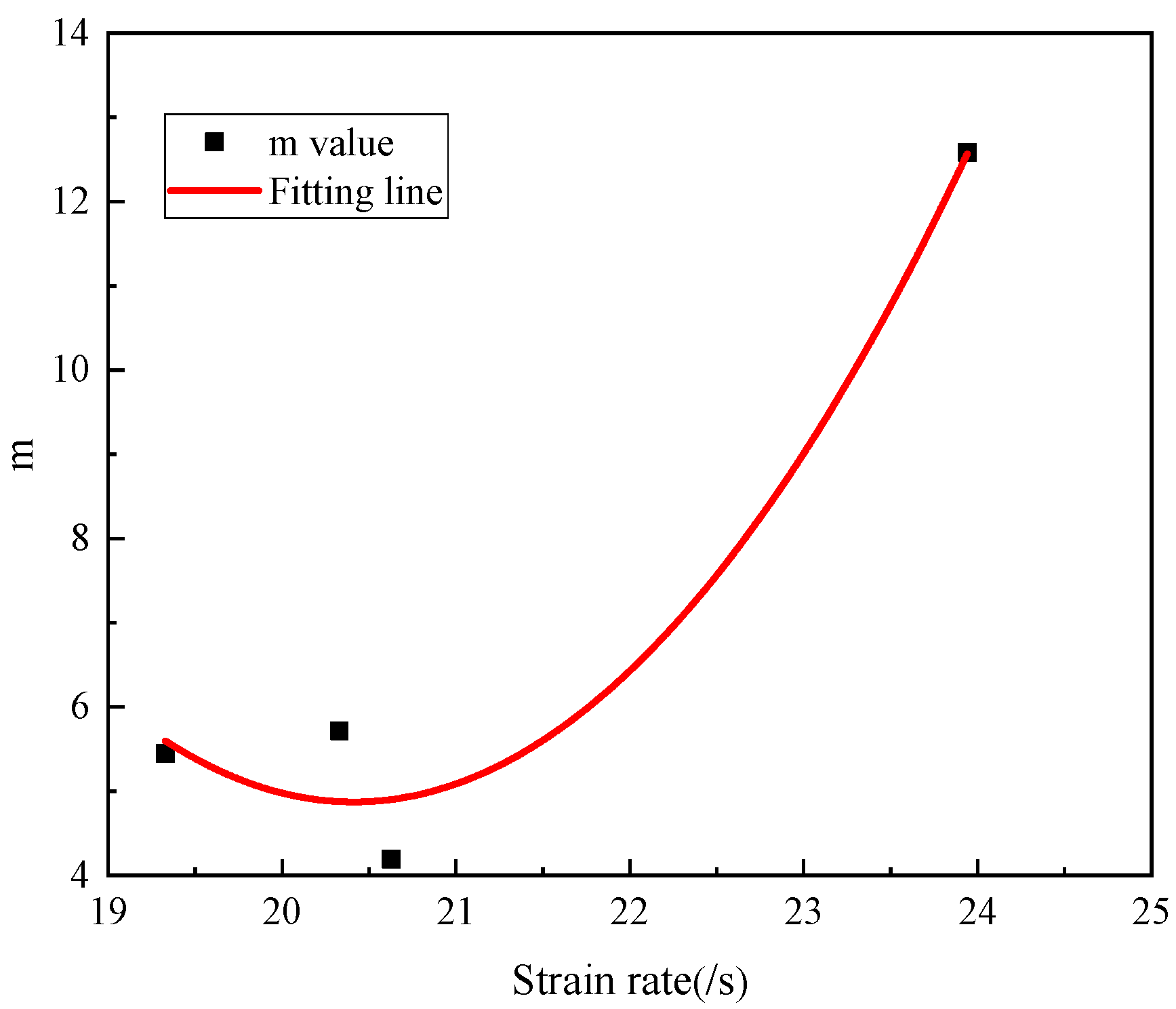
| Temperature | Strain Rate (s−1) | (MPa) | |
|---|---|---|---|
| 60 °C | 20.63 | 141.767 | 4.902 |
| 90 °C | 19.33 | 153.223 | 5.599 |
| 120 °C | 20.33 | 144.413 | 4.878 |
| 150 °C | 23.94 | 112.608 | 12.565 |
Disclaimer/Publisher’s Note: The statements, opinions and data contained in all publications are solely those of the individual author(s) and contributor(s) and not of MDPI and/or the editor(s). MDPI and/or the editor(s) disclaim responsibility for any injury to people or property resulting from any ideas, methods, instructions or products referred to in the content. |
© 2023 by the authors. Licensee MDPI, Basel, Switzerland. This article is an open access article distributed under the terms and conditions of the Creative Commons Attribution (CC BY) license (https://creativecommons.org/licenses/by/4.0/).
Share and Cite
Gao, W.; Deng, G.; Sun, G.; Deng, Y.; Li, Y. Dynamic Mechanical Properties of Heat-Treated Shale under Different Temperatures. Appl. Sci. 2023, 13, 12288. https://doi.org/10.3390/app132212288
Gao W, Deng G, Sun G, Deng Y, Li Y. Dynamic Mechanical Properties of Heat-Treated Shale under Different Temperatures. Applied Sciences. 2023; 13(22):12288. https://doi.org/10.3390/app132212288
Chicago/Turabian StyleGao, Weiliang, Guoqiang Deng, Guijuan Sun, Yongjun Deng, and Yin Li. 2023. "Dynamic Mechanical Properties of Heat-Treated Shale under Different Temperatures" Applied Sciences 13, no. 22: 12288. https://doi.org/10.3390/app132212288
APA StyleGao, W., Deng, G., Sun, G., Deng, Y., & Li, Y. (2023). Dynamic Mechanical Properties of Heat-Treated Shale under Different Temperatures. Applied Sciences, 13(22), 12288. https://doi.org/10.3390/app132212288