Abstract
The Gray Wolf Optimizer (GWO) is an established algorithm for addressing complex optimization tasks. Despite its effectiveness, enhancing its precision and circumventing premature convergence is crucial to extending its scope of application. In this context, our study presents the Cauchy Gray Wolf Optimizer (CGWO), a modified version of GWO that leverages Cauchy distributions for key algorithmic improvements. The innovation of CGWO lies in several areas: First, it adopts a Cauchy distribution-based strategy for initializing the population, thereby broadening the global search potential. Second, the algorithm integrates a dynamic inertia weight mechanism, modulated non-linearly in accordance with the Cauchy distribution, to ensure a balanced trade-off between exploration and exploitation throughout the search process. Third, it introduces a Cauchy mutation concept, using inertia weight as a probability determinant, to preserve diversity and bolster the capability for escaping local optima during later search phases. Furthermore, a greedy strategy is employed to incrementally enhance solution accuracy. The performance of CGWO was rigorously evaluated using 23 benchmark functions, demonstrating significant improvements in convergence rate, solution precision, and robustness when contrasted with conventional algorithms. The deployment of CGWO in solving the engineering challenge of pressure vessel design illustrated its superiority over traditional methods, highlighting its potential for widespread adoption in practical engineering contexts.
1. Introduction
The swarm intelligence algorithm comprises a variety of computing methods inspired by group behavior in nature, and its central premise is to solve diverse problems by simulating the cooperative work among the individuals of a given population [1]. In recent years, with the introduction of the particle swarm algorithm [2] and other algorithms, many scholars have focused their energy on this research field. Currently, the swarm intelligence algorithm has been widely used in academia and various engineering disciplines.
The Gray Wolf Optimizer (GWO), an intelligent global optimization method, was proposed by Mirjalili in 2014 [3]. This algorithm, predicated on the cooperative hunting behavior and hierarchical structure of gray wolves in nature, has since garnered substantial academic interest. It has seen widespread application in computer science [4], engineering science [5], energy science [6], biomedical science [7], and other fields.
GWO has been utilized as an optimization tool in diverse areas. For instance, Zaid et al. [8] employed it for intelligent fractional integral control to achieve load frequency control in a two-zone interconnected modern power system. Azizi et al. [9] leveraged a multi-objective variant of GWO to determine the optimal operating conditions of a novel cogeneration system. Ullah et al. [10] adopted GWO when optimizing the parameters of an electric vehicle charging time prediction model. Moreover, Wang et al. [11] utilized it to optimize parameters in an energy prediction model to predict the energy development trend in the next few years. Elsisi [12] utilized an improved version of GWO for an adaptive predictive model for the control of autonomous vehicles, and Shaheen et al. [13] employed it for grid-wide optimal reactive power scheduling. Furthermore, Hu et al. [14] and Boursianis et al. [15] both demonstrated GWO’s utility in the prediction of wind speed and the optimization of antenna design and synthesis, respectively. Liu et al. [16] incorporated the Gray Wolf Optimizer (GWO) algorithm into the domain of robotic path planning. Through the integration of a suite of enhancement techniques, this approach facilitated notable advancements in the practical application of path planning, thereby offering a more efficacious optimization strategy that contributes significantly to the progression of research in robotic path planning.
Although the GWO algorithm has many advantages, there are still some problems. Since it is centralized when hunting under the leadership of three wolves, when the leading wolf falls into the local extremes, other individuals are also affected. Therefore, when solving some large-scale problems, this algorithm is hindered by a lack of diversity and can easily fall into the local optimum [17]. To this end, many studies related to GWO have been proposed. Meidani et al. [18] proposed an adaptive GWO, which adaptively adjusted the convergence factor based on fitness in the search process to improve the performance of the algorithm. Zhang et al. [19] proposed two dynamic GWO algorithms based on the standard GWO. The position update of the current search wolf does not need to wait for the comparison between other search wolves and the three leading wolves; therefore, it can update the position in time and improve the speed of iterative convergence. Sun et al. [20] proposed an equilibrium Gray Wolf Optimization algorithm with refracted reverse learning, which overcame the problem of the low population diversity of GWO groups in the later stage and reduced the possibility of falling into local extremes. Li et al. [21] introduced a differential evolution algorithm and nonlinear convergence factor into the traditional GWO algorithm to solve the problem that the algorithm can easily fall into the local optimum. Zhou et al. [22] proposed a nonlinear convergence factor and search mechanism so that, when hunting, the update of the wolf pack is not only affected by the three leading wolves but also by the position of the surrounding wolves.
The optimization ability of the above improved GWO algorithm has been enhanced to some extent, but there are still some limitations. For example, Dereli [23] proposed an improved convergence factor, which improved the accuracy of the algorithm; however, the problem of insufficient diversity in the later stage remained. Heidari and Pahlavani [24] adopted Levi flight and greedy strategies, which can improve the ability of the GWO algorithm to jump out of the local optimum when solving many multimodal problems but did not accelerate the convergence speed. Based on the above shortcomings, this paper proposes a series of strategies to improve GWO based on the long tail property of Cauchy distribution. First, an initialization strategy that follows a Cauchy distribution is used to increase the diversity of the initial population. Secondly, a dynamic nonlinear inertia weighting strategy based on Cauchy distribution and logarithmic function is proposed to further improve the search performance of the algorithm. Finally, in the late iteration of the algorithm, the inertia weight is taken as the key index to measure mutation probability, and a Cauchy mutation operator is introduced to update the position to improve the population diversity and greatly improve the ability of the algorithm to jump out of the local optimum. The Cauchy distribution’s introduction to GWO enhances the algorithm’s global search ability, maintains diversity within the population, and provides a dynamic balance between exploration and exploitation, which, collectively, solve the issues of premature convergence and limited late-stage search diversity. Simulation results show that CGWO has great advantages in terms of solution accuracy, convergence speed, and stability.
The quest for optimal solutions in diverse engineering design scenarios has long stood as a pivotal challenge in the realm of industrial production. With the ongoing evolution of optimization technology, significant advancements have been achieved in addressing complex, real-world engineering conundrums [25]. Furthermore, a plethora of novel optimization methodologies have been effectively integrated into a myriad of engineering design processes [26]. Among these, the design of pressure vessels is recognized as a quintessential problem [27], with the primary objective of minimizing overall design costs. In this context, selecting an optimization technique that aptly balances exploratory and developmental aspects, while, concurrently, circumventing local optima, is of paramount importance. This paper introduces the application of the newly proposed Cauchy Gray Wolf Optimizer (CGWO) algorithm to this specific design challenge. The results pertaining to pressure vessel design underscore the formidable potential of CGWO in navigating the complexities inherent in practical engineering issues, thereby heralding a novel avenue for resolving intricate challenges in engineering design optimization.
The rest of the paper is structured as follows: Section 2 describes the related work. Section 3 describes the details of the proposed CGWO algorithm and the algorithm flow. Section 4 shows the results and analysis of the simulation experiments on 23 standard test functions. Section 5 implements CGWO to a fundamental engineering task: the design of pressure vessels. Section 6 provides the conclusions.
2. Related Work
2.1. An Overview of the Gray Wolf Optimizer
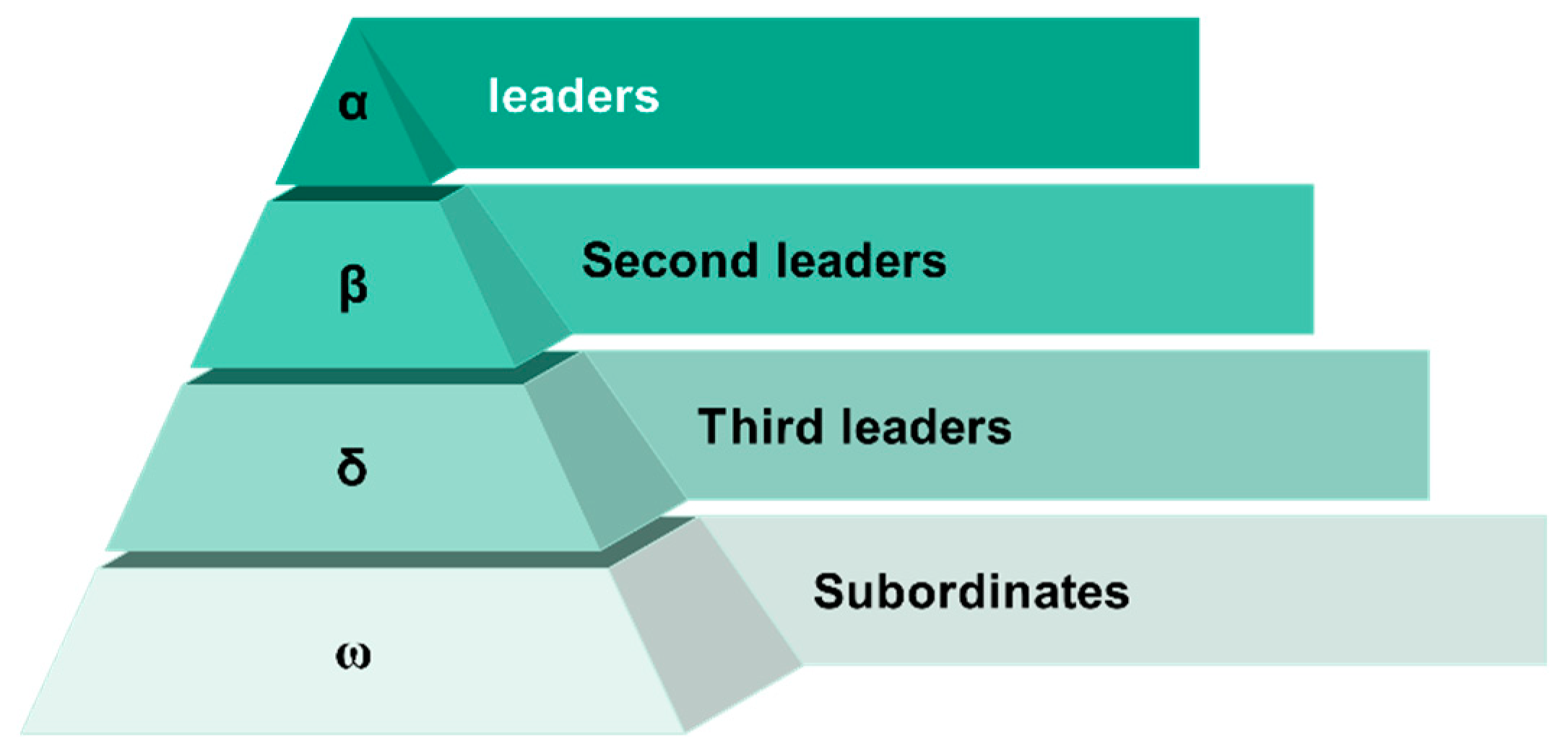
The Gray Wolf Optimization algorithm simulates the hierarchical structure of the gray wolf population and its hunting behavior in nature. Hierarchy is the main characteristic of the gray wolf pack, and, to maintain order in the wolf pack, the gray wolf population is divided into four levels, namely, α, β, δ, and ω wolves, as shown in Figure 1.
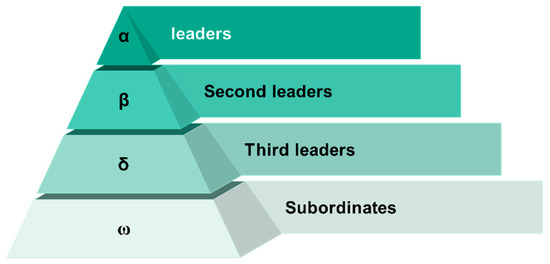
Figure 1.
Chart of ranks.
In Figure 1, each wolf plays a different role in the group, among which α, β, and δ are considered to be the leader wolves with better ability, representing the optimal value, the second-best value, and the third-best value, respectively.
The gray wolf’s hunting process consists of three main steps, namely, finding the prey, surrounding and hunting until it stops moving, and, finally, attacking it. The process of encirclement can be modeled by updating the position of each wolf relative to that of the prey, as in Equation (1):
where and are the position vectors of prey and gray wolf, respectively, is the distance vector, and is the current number of iterations.
Update the wolf’s position in the next iteration as shown in Equation (2):
and in Equations (1) and (2) are coefficient vectors, and their calculation formula is shown in Equation (3):
where and are random numbers in the range [0, 1]; is the convergence factor, which decreases linearly from 2 to 0 in iterations. The calculation formula of is shown in Equation (4):
where is the maximum number of iterations.
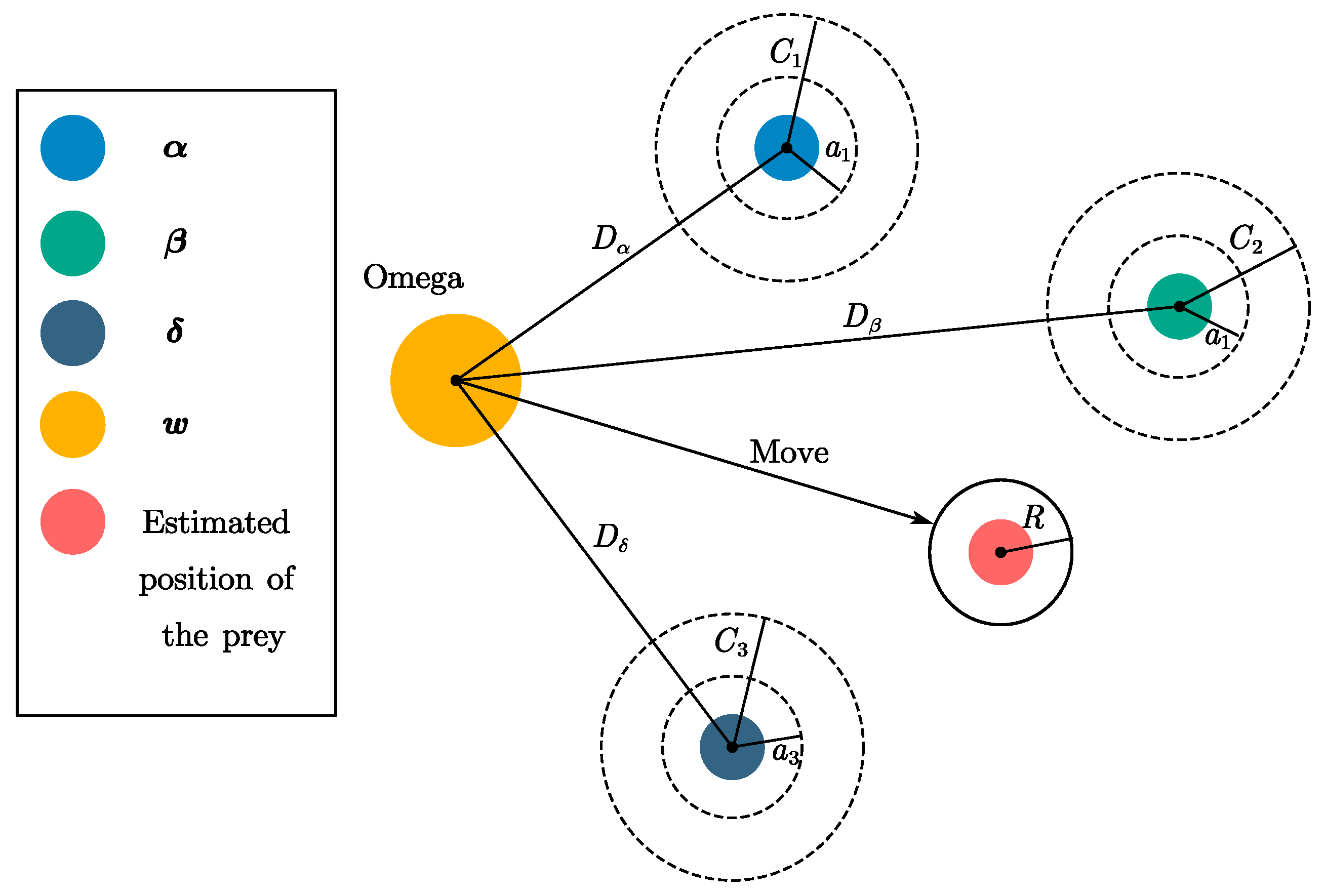
In the decision space of the optimization problem, the best solution (the position of the prey) is not known. Therefore, in order to simulate the hunting behavior of the gray wolf, α, β, and δ are assumed to know the potential position of the prey better, and the positions of the three are used to judge the position of the prey so that other gray wolves update their positions according to the positions of the three optimal gray wolves and gradually approach the prey, as shown in Figure 2.

Figure 2.
Schematic diagram.
The mathematical formula for calculating the distance vector of the three leading wolves during the gray wolf hunting the target prey is shown in Equation (5):
where , , and signify the respective distances from the α, β, and δ wolves to the other members of the pack. Correspondingly, , , and denote the present position vectors of the α, β, and δ wolves, and designates the current position vector of the gray wolf under consideration. Moreover, , , and are vectors composed of random coefficients.
The formula for the position update of the ω wolf is shown in Equation (6):
where , , and denote the current positions of the three wolves, respectively. , , and are vectors composed of random coefficients.
2.2. Cauchy Distribution
The Cauchy distribution, also known as the Cauchy—Lorentz distribution, is a continuous probability distribution [28]. It has some special properties, such as heavy tails. This makes Cauchy distribution better able to capture the occurrence of extreme values and is suitable for describing some abnormal situations or rare events [29]. The probability density function of the Cauchy distribution is shown in Equation (7):
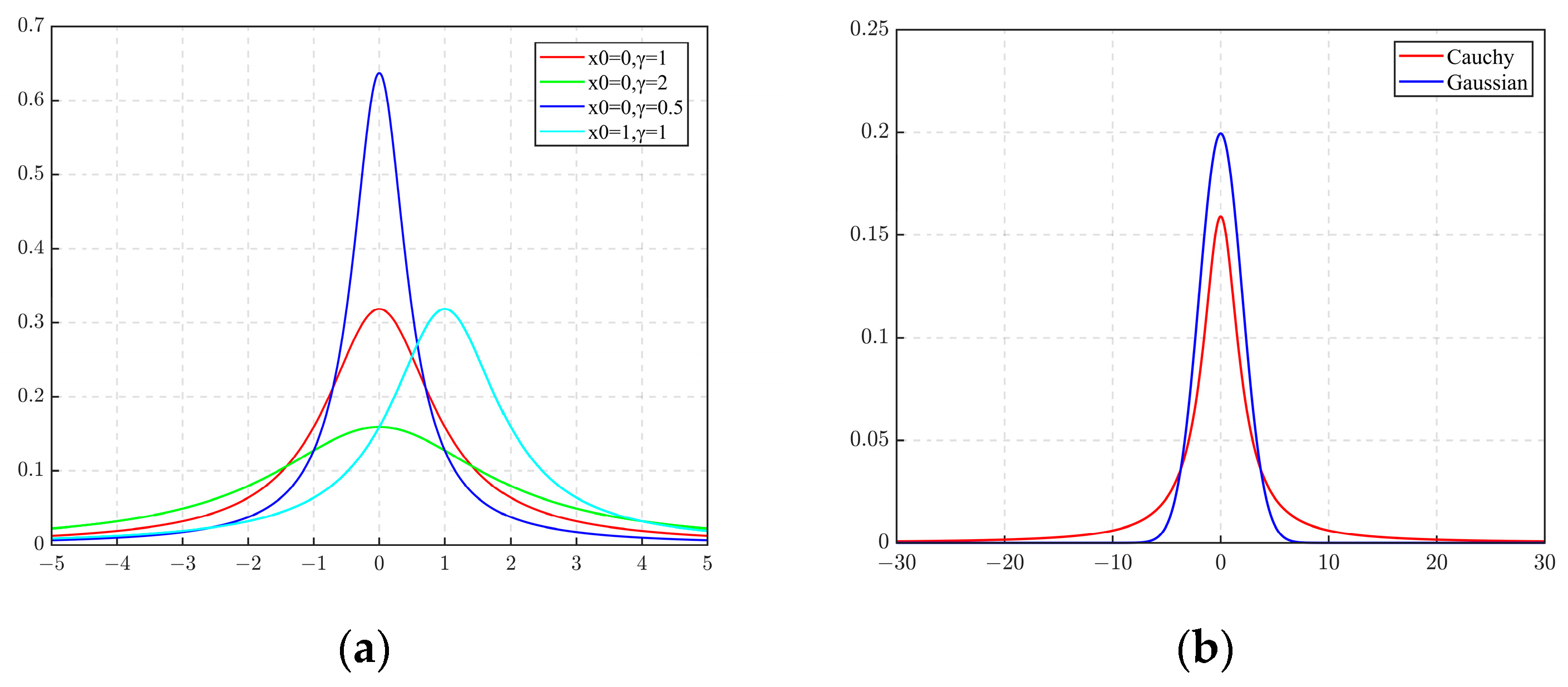
where is the location parameter, which can control the location of the distribution. is the scale parameter [30], which can control the shape of the distribution. In order to understand the Cauchy distribution more intuitively, the distribution curve of the Cauchy distribution with different parameters and the comparison between the Cauchy distribution and Gaussian distribution curves are drawn, as shown in Figure 3.
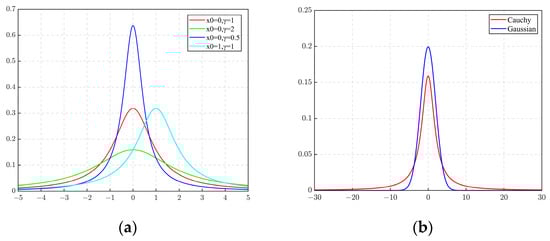
Figure 3.
Cauchy distribution graph: (a) Graphs of different parameters; (b) Comparison of Cauchy distribution and Gaussian distribution among them. The red curve in Figure 3 is the standard Cauchy distribution.
It can be seen from Figure 3 that the Cauchy function curve is a symmetric bell-shaped curve, which slowly decreases from the top to the two ends. The peak distribution of the Cauchy distribution at the origin of the coordinates is shorter, and the rest of the peak distribution is longer. In comparison to the Gaussian distribution, the Cauchy distribution exhibits a broader spread and a more pronounced propensity for dispersion [31], endowing it with the ability to produce outlier values at considerable distances from the mean. Luo [32] has observed that, while the Gray Wolf Optimizer (GWO) demonstrates exemplary efficacy in resolving optimization problems with global optima situated at the coordinate origin, its performance is marred by a marked search bias in scenarios where the optima deviate from this central point. Such an association demonstrably underscores the efficacy and logical foundation underlying the employment of the Cauchy distribution as a strategic enhancement of the GWO algorithm.
Building on the foregoing analysis, the incorporation of the Cauchy distribution within the Gray Wolf Optimizer (GWO) algorithm is hypothesized to bolster its explorative prowess while simultaneously diminishing the tendency for premature convergence to local optima. Consequently, the heavy-tailed nature of the Cauchy distribution is of considerable significance in the sophisticated augmentation of the established GWO paradigm.
The cumulative distribution function of the Cauchy distribution is shown in Equation (8):
The formula [33] for generating random numbers using Cauchy distribution is shown in Equation (9):
where is a random number in the range from 0 to 1.
Since the slope of the tangent function tan increases at a very fast rate, Cauchy random numbers have a probability of some extreme values, and the randomness is greater. If the optimal solution of the problem occurs, in some extreme cases, the use of Cauchy random numbers is advantageous. When the algorithm falls into the local optimum, the mutation of random numbers has a greater probability of jumping out of the local optimal solution. Based on the above characteristics of Cauchy distribution and Cauchy random numbers, the basic GWO algorithm is improved.
3. The Proposed Algorithm
3.1. Introduction of the CGWO
To solve the search bias of the traditional GWO that occurs when solving the problem that the optimal solution is not at the origin, this paper makes a series of improvements to the traditional GWO algorithm based on the characteristic that the Cauchy distribution has a greater probability to generate extreme values far from the origin compared with other distributions.
Improvements are mainly made from the following three aspects:
- (1)
- An initialization strategy predicated on the Cauchy distribution is implemented. Leveraging the heavy-tailed nature of the Cauchy distribution, the scope of distribution for the initial individuals is broadened, thereby circumventing an overly concentrated distribution of initial individuals that could lead to entrapment in local optima. This enhancement in the initialization process, achieved through the augmentation of the initial population’s diversity, enables the algorithm to conduct a more extensive search in its initial stages, thereby significantly bolstering its global search capabilities;
- (2)
- Employing a dynamic, nonlinear hybrid weighting strategy, which integrates the Cauchy distribution and logarithmic functions and facilitates a time-responsive adaptation of the algorithm’s search mechanism. This adaptation aligns with the distinct characteristics prevalent in different phases of the search process. In the initial stages, this strategy significantly enhances the algorithm’s capability for global exploration, whereas, in the latter stages, it effectively accelerates the convergence rate. Such a strategic approach ensures a more nuanced balance between global and local search methodologies at each stage of the algorithm’s execution, thereby optimizing overall performance;
- (3)
- The Cauchy mutation strategy based on dynamic inertia weights was adopted to improve the position update, and the Cauchy distribution was introduced in the late search period to generate certain disturbances to individuals. Meanwhile, the controllability of disturbance control based on the survival of the fittest rule improved the diversity of the late population within a controllable range and enhanced the ability of the algorithm to break out of the local optimal value.
3.2. Cauchy Initialization Strategy
The GWO algorithm adopts a random method to initialize the population, and the evolution of the population is only guided by the better solution in the population, which makes the GWO algorithm easily fall into the local optimal value [34].
In order to avoid the excessive concentration of initialized individuals and poor global search ability, combined with Cauchy random numbers [35], this paper proposes a Cauchy initialization strategy, as shown in Equation (10):
where is the lower bound of the variable, is the upper bound, and is the random number based on the Cauchy distribution.
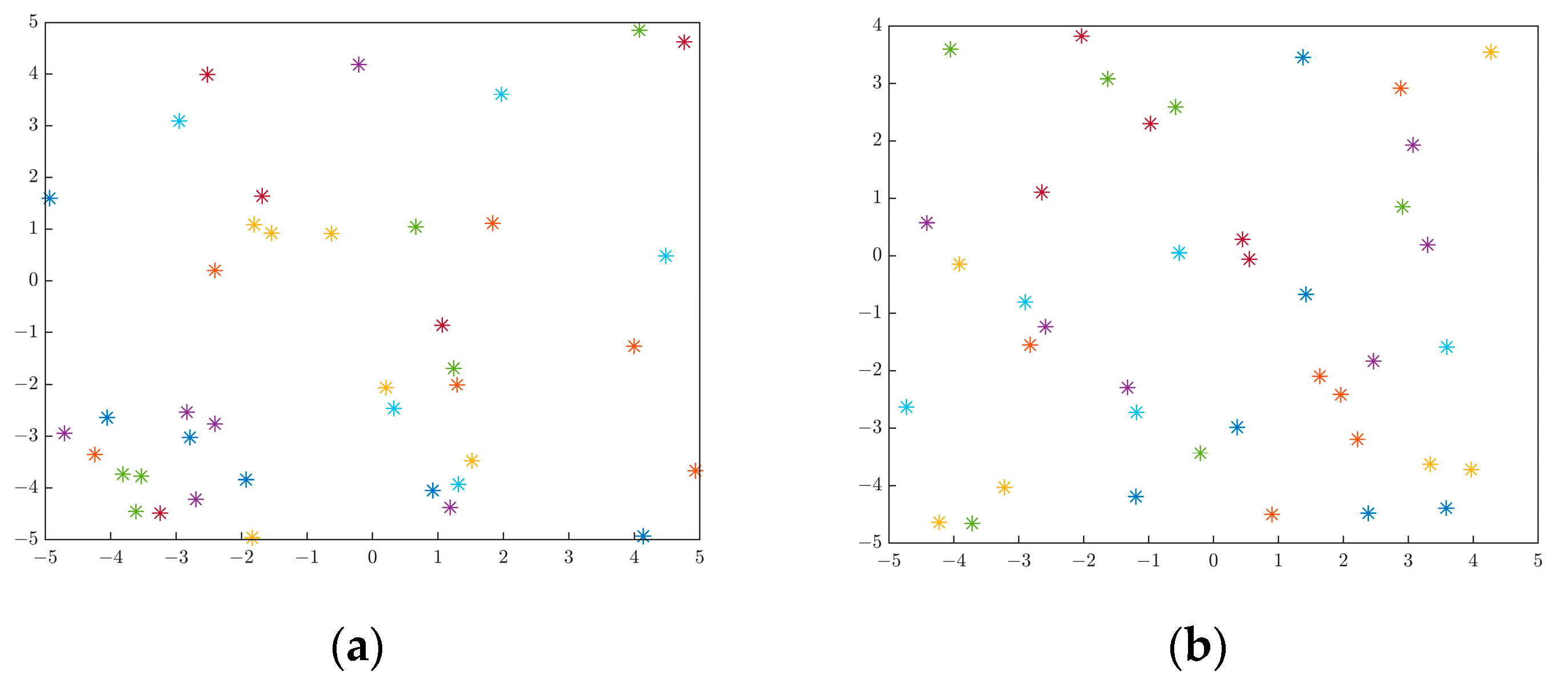
The distribution of the initial population in the search space plays a key and decisive role in the global search ability of the algorithm. Compared with the initial population distribution of the conventional random method, the introduction of the random numbers generated by the Cauchy distribution can improve the initial diversity of particles, and this diversity helps the algorithm avoid a premature concentration in the search space to obtain more exploration in the search process. The comparison between random initialization and Cauchy random initialization is shown in Figure 4.

Figure 4.
Comparison of random initialization and Cauchy random initialization: (a) random initialization; (b) Cauchy random initialization.
Figure 4 shows the scatter plots of the conventional random initialization and the Cauchy random value initialization proposed in this paper. It can be seen from the figure that the conventional random point selection may cause the initial individual distribution to be more concentrated, thus making the algorithm more likely to fall into the local optimum. Individuals are more likely to be created far from the center so they can cover most of the search space [36], which improves the diversity of the initial population and reduces the possibility of the algorithm falling into the local optimum.
3.3. Dynamic Nonlinear Inertia Weights Based on Cauchy Distribution
Shi and Eberhart [37] proposed an inertial weight method in particle swarm optimization that made outstanding contributions to the balance between algorithm exploration ability and development ability. Since GWO can easily fall into local optima, the idea of inertia weight has been introduced into GWO to improve its performance [38,39].
In order to improve the optimization ability of GWO, and inspired by the improved inertia weight of the PSO algorithm [40], this study designs a dynamic nonlinear inertia weight that combines the Cauchy random number and logarithmic function. In order to balance the exploration ability and development ability, previous research shows that the inertia weight should be decreasing [41] and that the early ω value is large, which improves the global search ability of the algorithm. The value of ω decreases in the later period, which is aimed at the local search ability of the algorithm. However, when ω is very small in the later period, there is a loss in population diversity and the algorithm is susceptible to easily falling into the local optimum. In order to solve this problem, this paper introduces the Cauchy random value and proposes a dynamic and more flexible weight that not only realizes the nonlinear reduction in inertia weight but also improves population diversity and prevents premature convergence. The inertia weight proposed is shown in Equation (11):
where and represent the maximum and minimum inertia weights, respectively; , that is, the number of current iterations divided by the maximum number of iterations. is a constant used to regulate the trend of weight reduction.
This formula combines the logarithmic function and Cauchy random number to optimize the algorithm, which not only realizes the overall trend of nonlinear decline but also increases the population diversity of the algorithm in the later stage because of the introduction of the Cauchy random number, which meets the necessary conditions for convergence and will not converge prematurely. The first half of the equation ensures that the inertia weight decreases nonlinearly through the logarithmic function , and the weight decreases gradually as increases. Cauchy random numbers are introduced into the second half of the formula. Due to the strong disturbance of the Cauchy distribution, the diversity of the population in the later stage is improved, the local optimal solution is avoided, the accuracy of the algorithm is improved, and the convergence speed of the algorithm in the later stage is accelerated.
The position update formula based on inertia weight is shown in Equation (12):
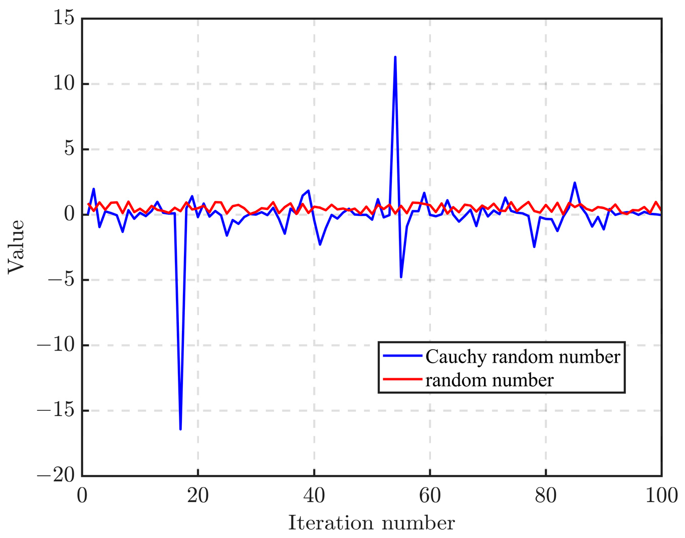
Equation (12) is modified by the application of a non-linear inertia weight governed by the Cauchy distribution, building upon the foundational position update Equation (6). This alteration transcends the realm of simplistic average calculations. During the position update procedure, the dynamic non-linear decay of the inertia weight enhances the equilibrium between exploration and exploitation, thereby expediting the algorithm’s iteration speed. The incorporation of Cauchy random numbers augments the algorithm’s diversity in the later stages, amplifying the likelihood of escaping local optima. Consequently, this formula amalgamates the advantageous properties of the Cauchy inertia weight into the position-updating process. By comparing the randomly generated numbers in 100 iterations with Cauchy random numbers, Figure 5 can be obtained.
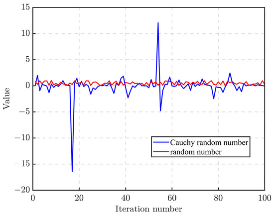
Figure 5.
Random numbers versus Cauchy random numbers.
It can be seen from Figure 5 that, compared with random numbers generated randomly, Cauchy random numbers have greater fluctuations and have a certain probability of producing some extreme values far from the origin, which is conducive to improving diversity and is better equipped to solve the problem that GWO can easily fall into the local optimum.
3.4. Cauchy Mutation Strategy Based on Dynamic Inertia Weight
Cauchy mutation, as an update strategy, has been applied to optimization algorithms by many scholars, and it has been proven to be an effective technique for improving algorithms [42]. Cauchy mutation can improve the exploration or development ability of the algorithm [43]. In this paper, the Cauchy nonlinear inertia weight is used as the mutation probability, and a new Cauchy mutation position update strategy combined with the inertia weight is proposed. Compared with the original position update strategy, the improved method can generate a wider range of individual mutations. Compared with the conventional Cauchy mutation strategy, the proposed mutation strategy is more flexible and can adapt to each stage of the search.
If the leading wolf is trapped in the local optimal value, other individuals will also be greatly affected. Therefore, the objects of the Cauchy mutation are the three leading wolves α, β, and δ. The Cauchy mutation strategy based on inertia weight is shown in Equation (13):
where is the individual before the mutation and is the individual after the mutation.
The mutation probability, which determines whether an individual needs mutation, is calculated using Equation (14).
In Equation (14), the inertia weight is taken as the mutation probability , which is the basis for judging whether the mutation operation is needed. In the early stage, the inertia weight remains at a large value, and the global search ability of the algorithm is strong. These perturbations are then added to the current position to generate new candidate solutions. The Cauchy distribution is a heavy-tailed distribution that does not have finite mean and variance; therefore, greater randomness can be introduced, which helps the algorithm jump out of the local optimum.
Due to the heavy-tail nature, the Cauchy mutation may also produce large disturbances. In order to prevent large disturbances from affecting the convergence speed, this paper first compares the fitness values of the mutant and the current optimal individual and then uses the survival of the fittest strategy [44] to determine the final new individual—this ensures that the perturbations generated by the Cauchy distribution are controllable. The specific position update formula is shown in Equation (15):
where is the fitness function value of the , and individual before the mutation, and is the fitness function value of the individual after the mutation. is the mutation probability, that is, the Cauchy inertia weight proposed in this paper, and it is a dynamically changing value.
Equation (15) uses the greedy strategy, which not only takes advantage of the long tail characteristics of a Cauchy mutation to increase population diversity in the later stage to prevent falling into the local optimum but also makes the mutant compete with the pre-mutation individuals according to the idea of natural selection, prevents accuracy decline in the algorithm caused by an extreme phenomenon in the Cauchy distribution.
3.5. The Pseudo-Code of the Proposed CGWO Algorithm
The pseudo-code of the proposed algorithm is shown in Algorithm 1.
| Algorithm 1 Pseudo-code of the CGWO |
| Initialize using Equation (10) to generate the gray wolf populations |
| Calculate the fitness valueof each individual in the population |
| Select the best individual |
| the second individual |
| the third individual |
| While t < maximum number of iterations |
| for |
| calculate the values of parameteraccording to Equations (3) and (4) |
| calculate the values of Inertia weightaccording to Equation (11) |
| update the position of individualsby Equations (6) and (12) |
| end |
| Update the leader wolf α, β and δ |
| If rand > Ps |
| use Cauchy mutation and survival of the fittest strategies to the leader wolves using Equations (13) and (15) |
| end |
| end |
In Algorithm 1, the initialization part is an improved initialization method based on the Cauchy random number, and the Cauchy nonlinear inertia weight is introduced in the position update part. In the later stage of the algorithm, the Cauchy mutation strategy and survival of the fittest law are used to increase the diversity of the population to avoid being trapped in the local optimum.
4. Simulation Experiment and Results Analysis
This paper includes five main experiments:
- (1)
- The first of the main experiments was conducted to find the appropriate values of the scale parameter of the Cauchy distribution and the parameter k of the inertia weight in the proposed algorithm, which can be used to select the parameters in the algorithm;
- (2)
- The second experiment is a comparison experiment between the proposed CGWO algorithm and several other optimization algorithms as well as traditional GWO, which is used to test the performance of CGWO in low and high dimensions;
- (3)
- The third experiment is a comparison between the inertia weight improvement strategy of this paper and the inertia weight strategy of several other proposed GWOs, which is used to test the effectiveness and superiority of the Cauchy inertia weight strategy;
- (4)
- The fourth experiment is a comparison of the proposed CGWO algorithm with several other improved GWO algorithms. It is used to verify the improvement in algorithm performance achieved by the improvements suggested in this paper;
- (5)
- The fifth experiment is a rank-sum test of the proposed algorithm against several algorithms in the first experiment. Through this test, one can test whether there is a significant difference between CGWO and other algorithms.
4.1. Experiment Set Up
The 23 benchmark function sets [45] employed in this investigation are of a classical nature and were rigorously selected to evaluate the Gray Wolf Optimizer (GWO) algorithm at its inception. The suite encompasses a tripartite categorization of test functions: 7 unimodal, 6 multimodal, and 10 fixed, low-dimensional multimodal benchmark functions. These functions are instrumental in assessing the multifaceted performance of an algorithm, amalgamating both its global optimization capabilities and local search proficiencies. The unimodal benchmark functions are typically harnessed to gauge the algorithm’s global search prowess and the performance on multimodal benchmarks is indicative of its local search efficiency and its susceptibility to premature convergence in local optima. To provide a holistic appraisal of the algorithm’s performance, the present study conducts evaluations across both lower and higher dimensions, thereby scrutinizing the algorithm’s scalability.
All the experiments were conducted on a PC using AMD Ryzen 7 5800H CPU and a Windows 10 operating system; in addition, all algorithms were run with MATLAB R2021a.
The unimodal benchmark function is presented in Table 1, where the function expression, dimensions, search range, and optimal solution are listed.

Table 1.
Unimodal reference function.
The multi-mode benchmark function is shown in Table 2.
Table 2.
Multimodal reference function.
The fixed-dimension, multimodal benchmark functions are shown in Table 3.
Table 3.
Fixed dimensional multimodal reference function.
4.2. Selection of Parameters
4.2.1. Selection of the Scale Parameter in the Cauchy Distribution
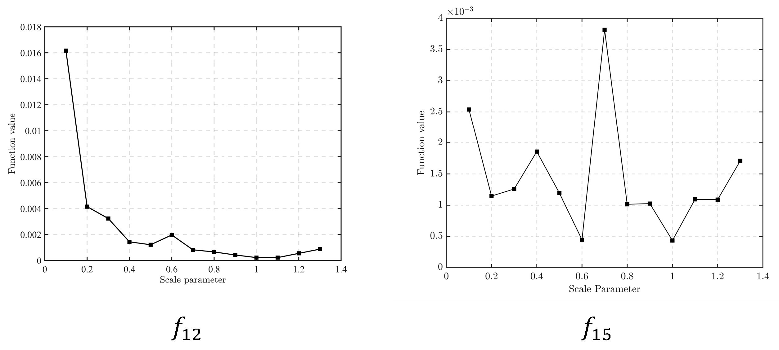
The scale parameter in the Cauchy distribution controls the shape of the Cauchy distribution, which has a certain impact on the exploration ability or development ability of the algorithm. Therefore, selecting the appropriate scale parameter is very important for the improvement effect. In order to obtain a reasonable value of , in this paper, a series of extensive experiments were carried out on the test functions in the table, and relatively consistent results were obtained. In brief, the mean values of the solution results of the algorithms with different values of on the five functions are given here. Among these four functions, and are unimodal benchmark functions, and are multimodal benchmark functions, and is a fixed-dimension, multimodal benchmark function. The experimental results are shown in Table 4, and the best experimental results are shown in bold.
Table 4.
The test results of CGWO with different values of .
From the analysis of the results in Table 4, for and , when the parameters are different, the results of this algorithm are consistent and good. For functions , , and , when the parameters are different, the results of this algorithm are not very different. When the value of is 1, the results of each function are good and the results are consistent. Therefore, the scale parameter of the Cauchy distribution is chosen as 1, which is also the parameter of the standard Cauchy distribution.
In addition, in order to intuitively show the influence of different values on CGWO performance, line charts showing the mean value of the algorithm solution results of and are presented in Figure 6:
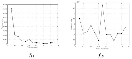
Figure 6.
Line plots of the results with different scale parameters.
As can be seen from Figure 6, for , when , the results of CGWO are more stable and accurate. For , when and , the results are good. Therefore, it is appropriate to set in the CGWO algorithm in this paper as the algorithm can better balance the abilities of exploration and development. It is also the parameter of the standard Cauchy distribution.
4.2.2. Selection of Inertia Weight Parameter
The parameter k of the logarithmic function of the dynamic inertia weight in CGWO can control the decreasing trend of the inertia weight. In order to obtain the appropriate parameter k value, this paper conducts a series of extensive experiments on the test functions in the table. For brevity, the results of four typical functions are shown. Among them, functions and are single-peak benchmark functions, is a multi-modal benchmark function, and is a fixed-dimension multi-modal benchmark function. The test results for parameter k are shown in Table 5, and the best experimental results in the table are shown in bold.
Table 5.
The test results of CGWO with different values of .
From the test results in Table 5, it can be analyzed that, for function , when the value of the parameter is different, the algorithm achieves the optimal result. For , the performance of the algorithm is relatively good after the value of is 4.0, and the effect is optimal when . For functions and , the algorithm performance is good in the range of the value; therefore, the value is determined to be 4.5.
In order to see the influence of different values more intuitively on the performance of the algorithm, a line diagram of the mean value of the algorithm solution results changing with the value is shown in Figure 7.

Figure 7.
Line plots of the results with different values of .
According to Figure 7 the following conclusions can be drawn. For function , the mean value solved using the algorithm shows a downward trend with the increase in the value of , and the results of the algorithm are better in the second half of the broken line, especially when . For and , it can be found from the figure that the results of the algorithm fluctuate to some extent with the change in the value of ; however, when is within the range of , the results of the algorithm are relatively better and more stable. Based on the above analysis, a value of 4.5 for is appropriate.
4.3. Effectiveness Test of CGWO: Comparison with Other Optimization Algorithms
In order to verify the performance of CGWO, this paper selects intelligent algorithms such as PSO, FA [46], FOA [47], GWO, and the proposed CGWO algorithm for comparison and analysis. The performance of all algorithms was evaluated according to the best value, mean value, and standard deviation generated by running the results on 23 test functions; for functions with non-fixed dimensions, the performance was tested with dimensions 30 and 100, respectively. These test statistics are presented below. The best experimental results in Table 6, Table 7 and Table 8 are shown in bold. Among them, the test results on the seven unimodal benchmark functions are shown in Table 6.
Table 6.
Test results for unimodal benchmark functions.
Table 7.
Multi−modal benchmark function test results.
Table 8.
Fixed−dimension, multimodal benchmark function test results.
It can be clearly seen from Table 6 that, for unimodal benchmark functions, the CGWO algorithm performs very well in both low and high dimensions. Specifically, for functions to , CGWO achieves the theoretical optimal value when the dimension is 30 and 100; moreover, the best value, mean value, and standard deviation are all 0, and the solution performance far exceeds that of other algorithms. For , the performance of CGWO and GWO is ahead of other algorithms, and there is little difference between CGWO and GWO in terms of solution accuracy, but the standard deviation of CGWO is better, indicating that the CGWO algorithm is more stable. For and , the performance of the CGWO algorithm is significantly better than that of the other four algorithms in both low and high dimensions, the results are up to 10 orders of magnitude higher than that of the other algorithms, and the best value, mean value, and standard deviation of CGWO are the best among the several algorithms. The unimodal benchmark function is usually used to test the global search performance of the algorithm, and the above analysis shows that the CGWO algorithm has a strong global search ability in both low and high dimensions.
The test results of the multi-modal benchmark function are shown in Table 7.
The test results in Table 7 show that CGWO has a strong solution performance in both low and high dimensions for multi-mode benchmark functions. For functions to the optimal value, mean value, and standard deviation of the CGWO test results in low and high dimensions are significantly better than those of the other four algorithms. Especially for and , CGWO reaches the theoretical optimal value, and the standard deviation and mean value are also 0. For , CGWO has better solution accuracy, and the calculated optimal value is closest to the theoretical optimal value. For , CGWO has the highest solution accuracy, and the order of magnitude of the results is 13 orders of magnitude higher than other algorithms. The above analysis is sufficient to show that CGWO has strong solution performance in the face of multimodal benchmark functions. The solution performance of the multi-mode benchmark function can usually reflect the local search performance of the algorithm and whether it has the disadvantage of falling into the local optimum. From the test results, CGWO has a good local search ability and the strongest ability to jump out of the local optimum solution, which is the result of making full use of the long tail characteristics of the Cauchy distribution, which proves the effectiveness of CGWO.
The test results of the fixed, low-dimensional multimodal benchmark function are shown in Table 8.
According to Table 8, for fixed dimension multi-mode benchmark functions, the solution performance of the CGWO algorithm also has good performance. For each test function, the optimal value of the CGWO results is closest to the theoretical optimal value, and the theoretical optimal value can be reached in most cases. Especially for functions to , the optimal value, mean value, and standard deviation of the CGWO results are the best. The excellent solution performance under the fixed dimensional multimodal benchmark function is enough to prove that CGWO can also perform a global search and jump out of the local optimum in a fixed, low-dimensional space excellently.
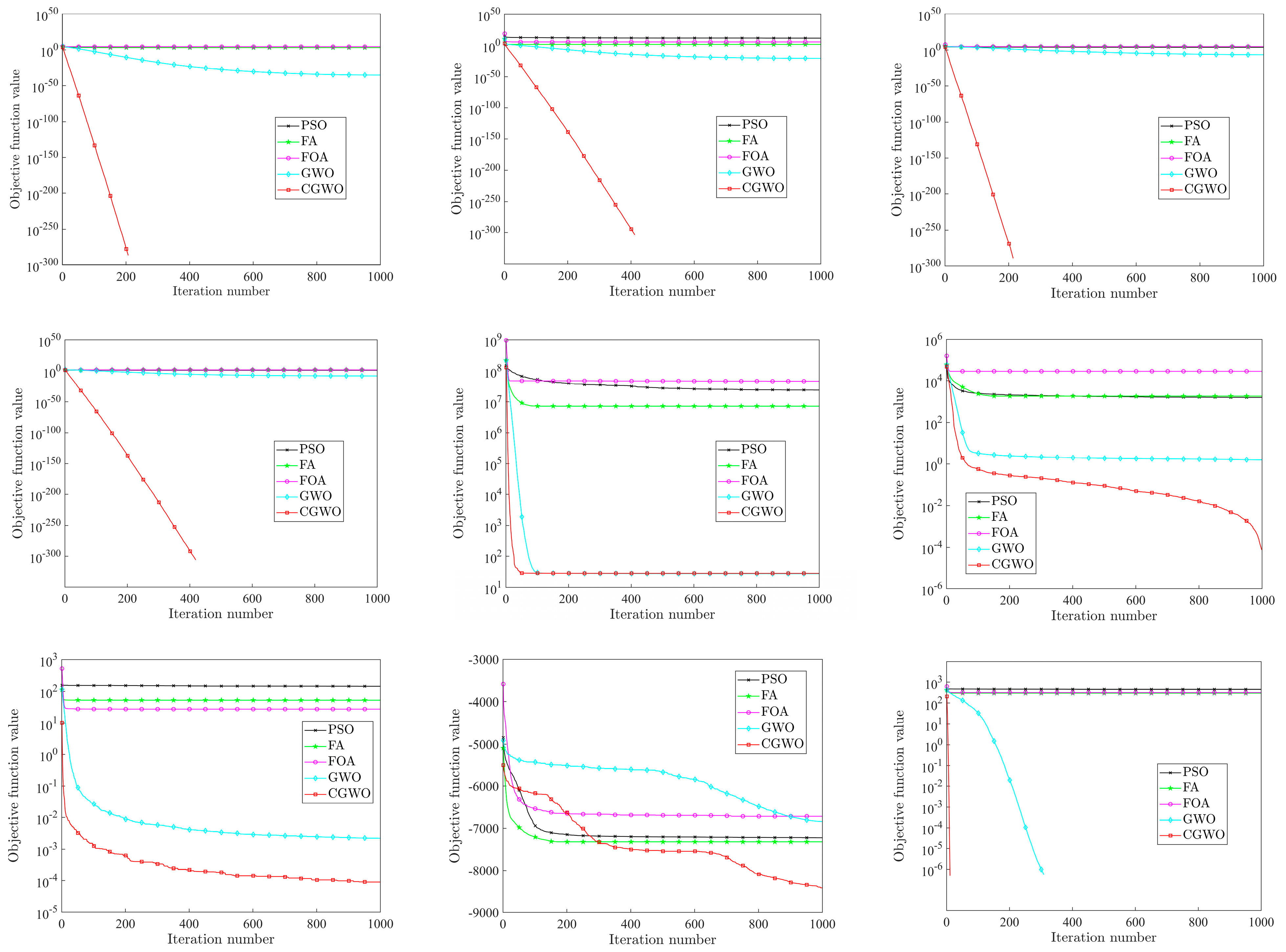
By analyzing the results of the above three categories of test functions (Table 6, Table 7 and Table 8), it can be concluded that CGWO has significant advantages in the accuracy, stability, and scalability of different types of test functions. In order to reflect the advantages of CGWO more intuitively, the convergence curves of the five algorithms for all test functions are shown in Figure 8.
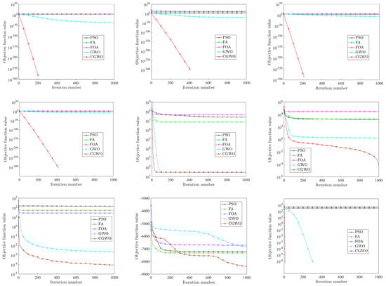
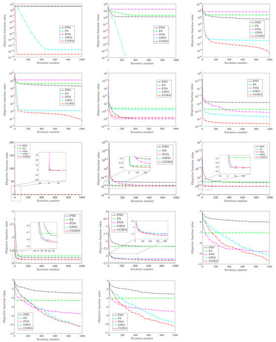
Figure 8.
Comparison of different algorithms.
By analyzing Figure 8, it can be found that the convergence speed of the CGWO algorithm is fast, especially for unimodal benchmark functions to and multi-modal benchmark functions to ; CGWO convergence speed is much faster than other algorithms: its accuracy is the highest, and it can quickly converge to the theoretical optimal value or the closest to the theoretical optimal value. It can be clearly seen from the iteration graphs of , , , and that, in the iteration process, CGWO jumps out of the local optimum value when other algorithms have an obvious tendency to fall into the local optimum, which reflects the excellent performance of CGWO in jumping out of the local optimum solution. Moreover, it fully reflects the advantages of the long tail characteristics of the Cauchy distribution. For , , and , although CGWO, like other algorithms, tends to fall into the local optimum, it has obvious advantages in solution accuracy and convergence speed compared with other algorithms, and the optimal value obtained is also closest to the theoretical optimal value. For , , and , CGWO, GWO, and FOA all have the ability to jump out of the local optimum; however, the accuracy and convergence speed of CGWO are better.
To sum up, CGWO has great advantages in accuracy, stability, scalability, and convergence, which fully verifies the feasibility and performance of the CGWO algorithm.
4.4. Validity Test of CGWO Inertia Weights: Comparison with Other Inertia Weight Strategies
In order to prove the effectiveness of the dynamic inertia weight based on the Cauchy distribution and logarithmic function proposed in this paper, three different types of inertia weights are selected from other improved Gray Wolf Optimizers (GWOs) in the literature for comparison. This paper calls the GWO algorithm improved by these three inertia weight strategies GWO1 [48], GWO2 [49], and GWO3 [50], respectively. The comparative test results of the algorithm improved by the Cauchy nonlinear weighting strategy and the GWO algorithm improved by these three weighting strategies are shown in Table 9, and the best experimental results are shown in bold.
Table 9.
The comparison results of four inertia weights.
As can be seen from Table 9, for the vast majority of test functions, the CGWO algorithm improved by the Cauchy nonlinear inertia weight has the best optimization performance. For each test function, the optimal value of the CGWO test results is the closest to the theoretical optimal value; in particular, functions to , , , , and to all reach the theoretical optimal value. For the vast majority of functions, the mean value and standard deviation of the CGWO results iarealso the best. Specifically, for and , only CGWO converges to the theoretical optimal value, while other algorithms cannot achieve the theoretical optimal value. For , , , and , CGWO outperforms the other algorithms by up to seven orders of magnitude. Through the experimental results of the Cauchy weight strategy, under the unimodal benchmark function, multi-modal benchmark function, and fixed-dimension, multi-modal benchmark function, it can be concluded that the proposed Cauchy nonlinear weight strategy can improve the global search ability of the algorithm, enhance the local search performance of the algorithm, and reduce the possibility of the algorithm falling into the local optimal solution. This fully demonstrates the advantage of the inertia weight strategy of the proposed CGWO in terms of solution performance.
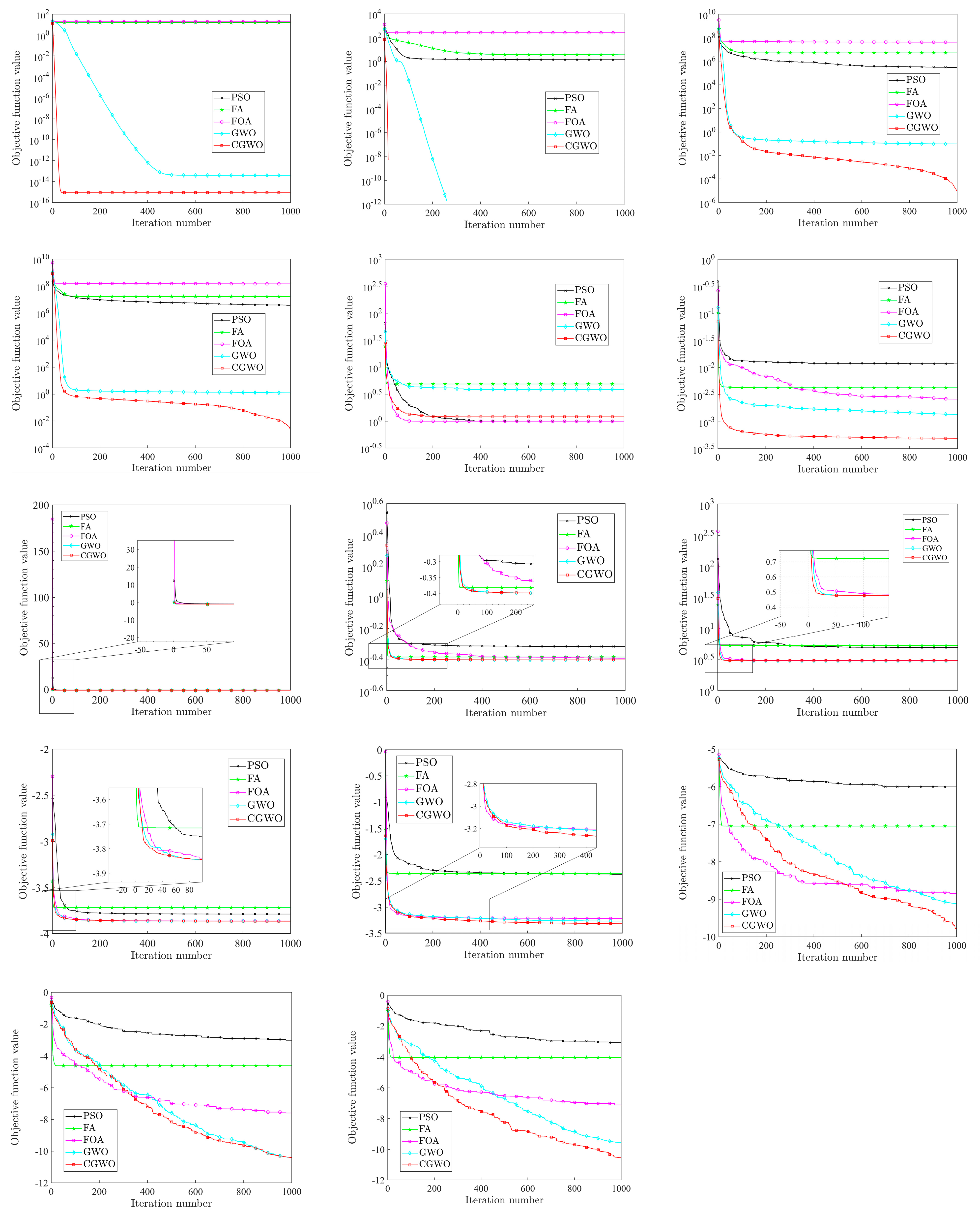
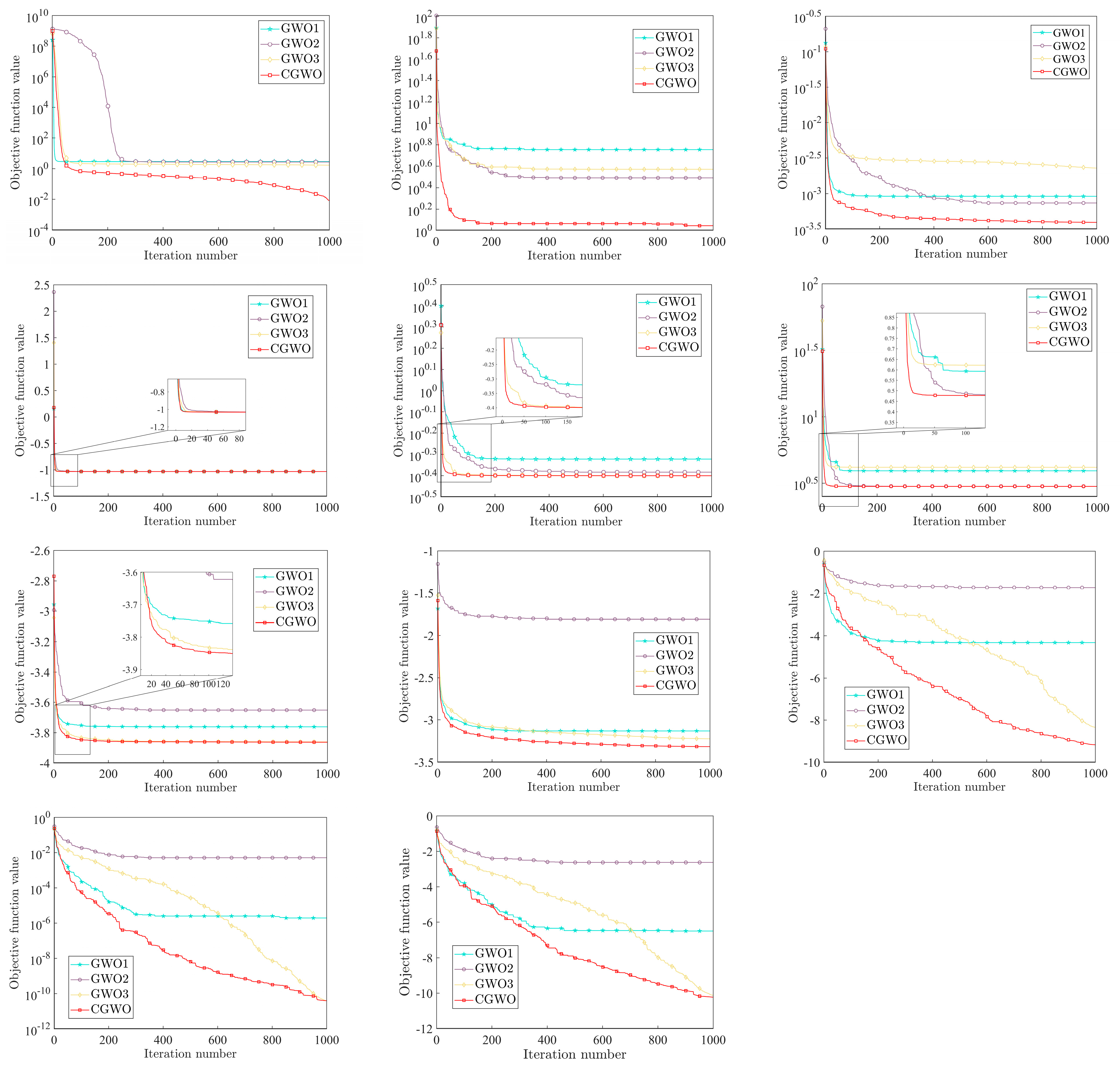
In order to compare the optimization effects of different inertia weight strategies more intuitively on the algorithm, the convergence curves of the four inertia weight strategies on all test functions are shown in Figure 9.
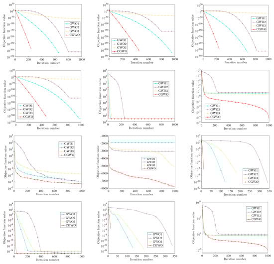
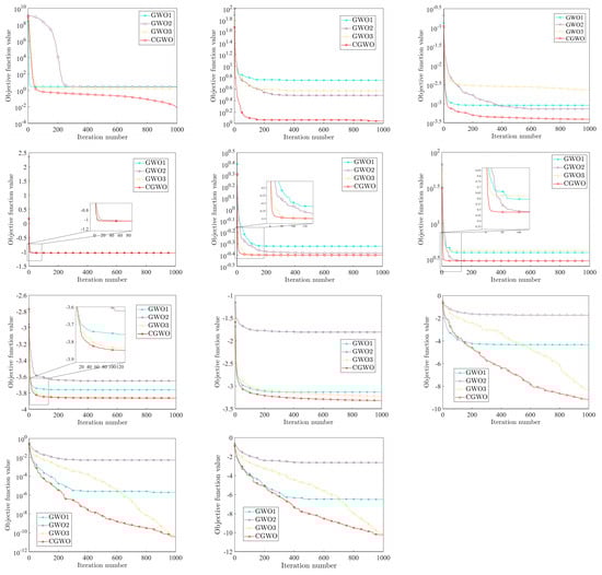
Figure 9.
Comparison of different weight strategies.
It can be seen from Figure 9 that the performance of CGWO under most test functions has obvious advantages over other algorithms, especially functions to , , , , and . For these functions, the convergence speed and solution accuracy of the CGWO algorithm are much higher than those of other algorithms. To be specific, for , , and , it can be clearly seen that, when the other three algorithms fall into the local optimum, CGWO breaks out of the local optimum in the iteration process, thus making the solution accuracy much higher than that of the other three algorithms. This fully reflects the advantages brought by introducing the long tail characteristic of the Cauchy distribution into the inertia weight, which improves the population diversity of the algorithm in the later stage. It also greatly improves the ability of the algorithm to jump out of the local optimum. For , , , and , although the four algorithms all tend to fall into the local optimum, the optimization ability of CGWO is still the best. For the multi-mode benchmark function and the fixed dimension multi-mode benchmark functions to , CGWO also has excellent performance, and the convergence speed is much faster than other algorithms, allowing for high solution accuracy and the ability to jump out of the local optimum.
To sum up, CGWO outperforms the other three algorithms in terms of accuracy, stability, and convergence, and CGWO has a strong ability to jump out of the local optimum, which shows that, for GWO, the Cauchy nonlinear dynamic inertia weight strategy has better performance than the other three inertia weights, reflecting the effectiveness and improvement of the proposed weight strategy.
4.5. Performance Comparison of CGWO with Several Other Improved GWOs
In order to further study the performance of CGWO, MGWO [51], HGWO [52], and LGWO [53], in this section, they were selected to compare these three improved GWO algorithms with the CGWO proposed in this paper. The implementation results are shown in Table 10, and the best experimental results are shown in bold.
Table 10.
The comparison results of MGWO, HGWO, LGWO, and CGWO.
As can be seen from Table 10, the CGWO algorithm proposed in this paper has the best performance for most of the unimodal benchmark functions, multi-modal benchmark functions, and fixed-dimension, multi-modal benchmark functions. Specifically, for unimodal benchmark functions to , the optimal value, average value, and standard deviation of the CGWO algorithm results are the best, among which, for functions to , only CGWO can achieve the theoretical optimal value with a mean value and standard deviation of 0, and the effect is excellent. For , although CGWO is the same as MGWO, HGWO, and LGWO, all fail to reach the theoretical optimal value; however, their optimal value is the closest to the theoretical optimal value and the most stable, reflecting the excellent global search ability of CGWO. For the multi-modal benchmark functions to , the three evaluation indexes of the CGWO results are also optimal, which reflects its strong local search ability and ability to prevent easily falling into the local optimum. For functions to , CGWO reached the theoretical optimal value. For several other multimodal benchmark functions, the CGWO results are up to five orders of magnitude higher than other algorithms, which is not only accurate but also the most stable. For fixed-dimension, multi-modal benchmark functions to , CGWO also has obvious advantages, with the highest solution accuracy and high stability, which proves that its solution ability is also excellent in multi-modal problems with fixed low dimensions. In general, the proposed improved CGWO outperforms the other three improved GWO algorithms in solving the unimodal benchmark function, the multi-modal benchmark function, and the fixed-dimension, multi-modal benchmark function.
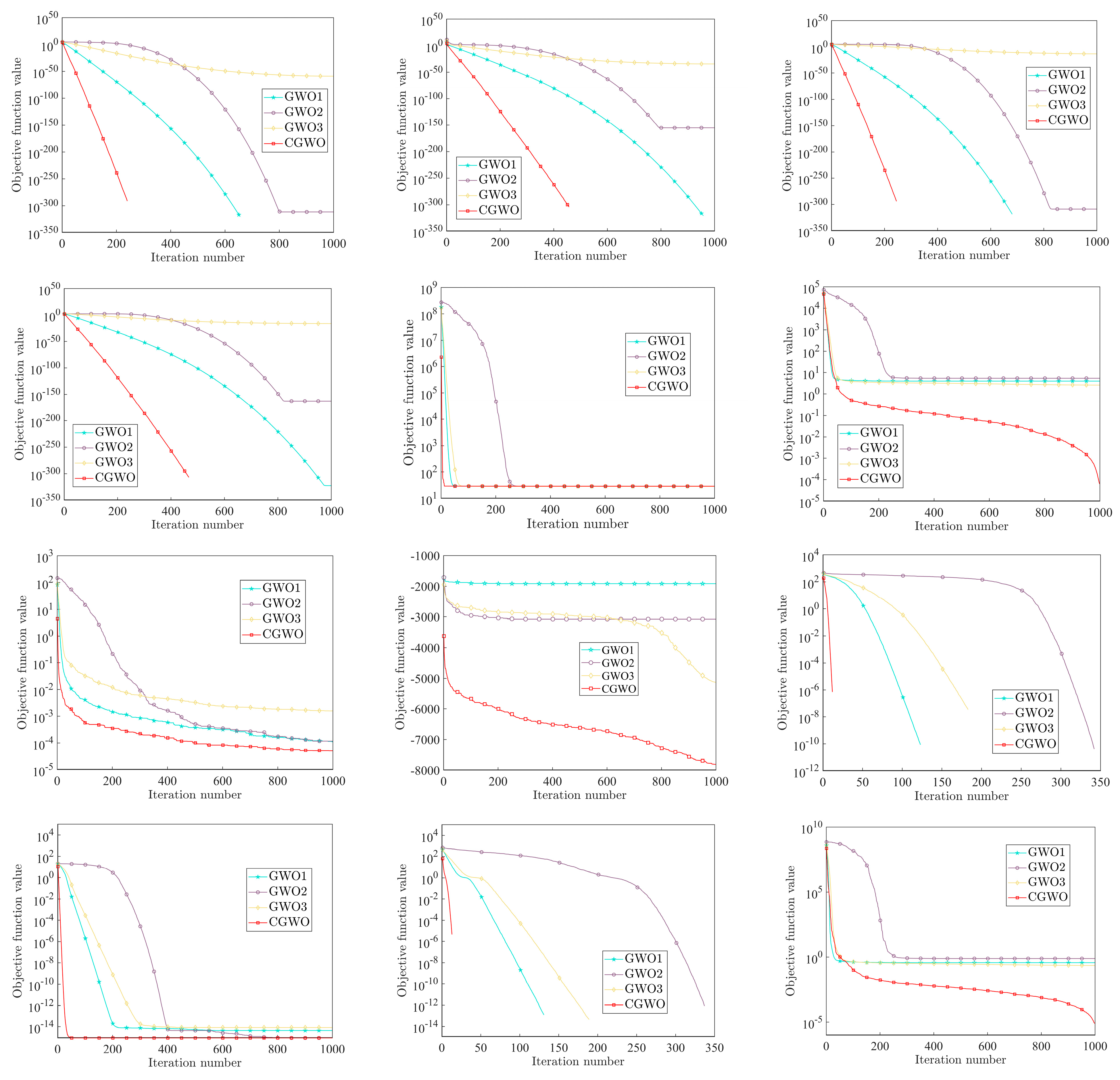
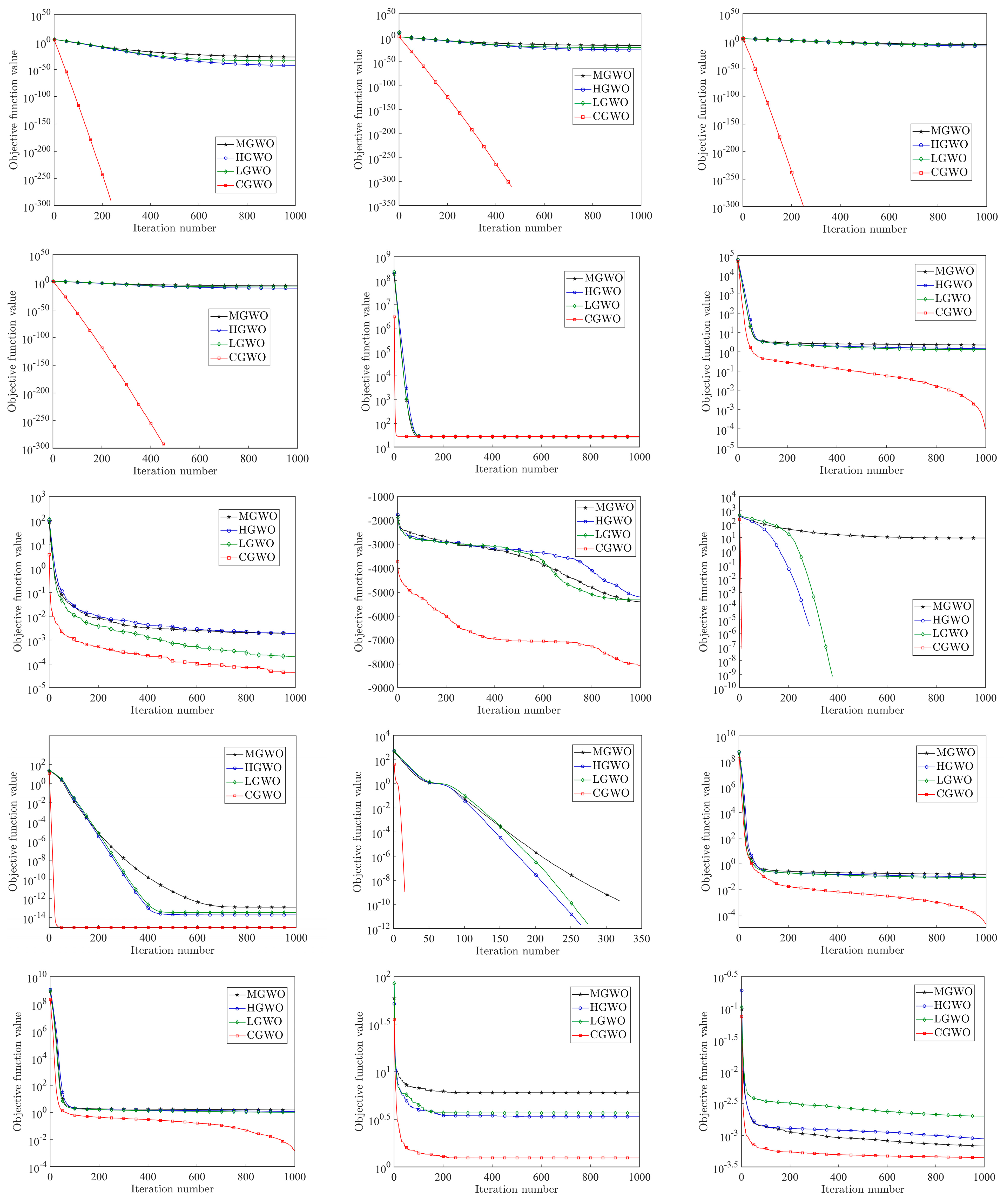
In order to further compare the performance of the four improved GWO algorithms, this paper draws the iterative convergence curves of the four improved algorithms under different test functions, as shown in Figure 10.
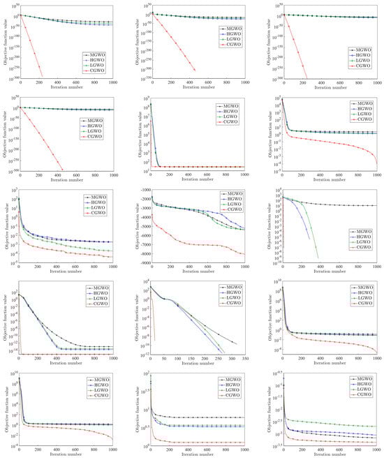
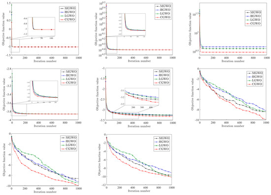
Figure 10.
Comparison chart of different improvements.
From Figure 10, it can be found that, for to , , and , CGWO has the fastest iteration speed and highest accuracy, and its performance far exceeds that of the other three improved algorithms. For , , and , CGWO can jump out of the local optimum when the other three improved GWOs fall into the local optimum solution, which fully reflects the ability of the Cauchy distribution to reduce the possibility of falling into the local optimum and proves that the improved idea in this paper can solve the problem that the traditional GWO algorithm can easily fall into the local optimum to a certain extent. For , , , , , and , although the change trends of the four improved algorithms are very similar, it can be seen that CGWO has a faster iteration speed and higher accuracy. For functions to , the four algorithms all have the ability to jump out of the local optimum under fixed low dimensions; however, the advantages of CGWO are more obvious and are reflected in its better iteration speed and accuracy. From the above analysis, it can be concluded that, among the four improved GWO algorithms, CGWO has a wider and better improvement effect, stronger search performance, faster iteration speed, and more stability.
4.6. Wilcoxon Rank Sum Test
In order to further evaluate the effectiveness and optimization performance of CGWO, this paper uses the Wilcoxon rank sum test to verify whether the running results of CGWO are significantly different from other algorithms at a significance level of a = 5% [54]; when p < a, hypothesis is rejected, indicating that there is a significant difference between the two algorithms. When p > a, hypothesis is accepted, indicating that there is no significant difference between the two algorithms. The test results of the CGWO, PSO, FA, FOA, and GWO algorithms at a significance level of a = 5% are shown in Table 11.
Table 11.
The rank sum test p−value.
As can be seen from Table 9, for most test functions, most of the p values of CGWO are less than the significance level a, and there are significant differences between the calculation results and the other four algorithms.
5. Solving a Pressure Vessel Design Problem
The design of pressure vessels represents a time-honored engineering challenge. The principal objective here is the cost optimization of cylindrical pressure vessels. The focus is on minimizing the manufacturing costs, which includes processes such as pairing, forming, and welding. A schematic representation of a pressure vessel is presented below.
As shown in the Figure 11, the pressure vessel’s top is hemispherical, and the design optimization variables include the length of the cylindrical section (, the inner radius (), the shell thickness (), and the head thickness (). These four variables are critical in pressure vessel design. The mathematical model of this problem is expressed as follows.

Figure 11.
Schematic diagram of pressure vessel structure.
Equation (16) constitutes the objective function of the classical pressure vessel design problem, delineating the minimization objective. This objective pertains to the discovery of an optimal configuration for the four design variables, namely, shell thickness Ts, head thickness Th, inner radius R, and cylinder length L. In the literature, this problem is solved by using the mathematical methods of an augmented Lagrangian multiplier [55] and branch-and-bound [56] classical techniques. This study utilizes intelligent optimization algorithms, namely, CGWO, PSO, FA, FOA, GWO, SCA, and WDO, to resolve the given problem. The outputs generated from these solutions are displayed in the succeeding table.
Table 12 shows that CGWO achieved the best results, which fully demonstrates its ability to obtain favorable outcomes in practical engineering problems.
Table 12.
The solution results from the pressure vessel design problems.
6. Conclusions
In this study, we introduce a refined Gray Wolf Optimization algorithm—CGWO—that was innovatively enhanced using the Cauchy distribution. This advancement is primarily aimed at overcoming the limitations of traditional GWO, such as its susceptibility to local optima and subpar optimization accuracy. Capitalizing on the long -tail characteristic of the Cauchy distribution, the CGWO algorithm incorporates an initialization strategy to broaden the search space from the outset. Moreover, by integrating a dynamic, nonlinear inertial weight strategy derived from both the Cauchy distribution and logarithmic functions, CGWO adeptly adapts to the distinct stages of the optimization process. This approach ensures a more effective balance between global and local searches, thereby mitigating the likelihood of converging on local optima and facilitating a swifter rate of convergence.
A key feature of CGWO is the implementation of a Cauchy mutation strategy, guided by dynamically changing inertia weights that serve as probabilities for mutation. In the algorithm’s later stages, this strategy enhances population diversity, harnessing a survival-of-the-fittest approach to control the disturbances induced by Cauchy mutations. This aspect significantly aids the algorithm in escaping local optima, thus improving both the accuracy and convergence speed.
To validate the enhancements proposed in this paper, CGWO was rigorously tested against 23 standard test functions from various perspectives. Comparative analysis with other optimization algorithms and improved GWO variants revealed that CGWO exhibits superior optimization capabilities and faster convergence, with the Cauchy dynamic strategy outperforming other inertial weight strategies. Further substantiation through the Wilcoxon rank-sum test established CGWO’s significant improvements over several competing algorithms, highlighting the efficacy and potential of our proposed enhancements in refining the basic Gray Wolf Optimizer and reducing the risk of entrapment in local optima.
Applying CGWO to a classical real-world engineering problem (specifically, pressure vessel design), the algorithm demonstrated notable effectiveness, suggesting its viability for complex engineering challenges. This indicates promising prospects for CGWO in addressing practical optimization problems, underscoring the feasibility and impact of our improvement strategy.
Future work will focus on a more comprehensive and in-depth performance evaluation of CGWO. Additionally, exploring its application in areas such as power system energy load prediction, autonomous vehicle fault diagnosis, and optimal path planning presents intriguing avenues for further research.
Author Contributions
Conceptualization, K.S.; Data curation, J.L.; Formal analysis, J.L.; Funding acquisition, K.S.; Methodology, J.L. and K.S.; Project administration, K.S.; Resources, K.S.; Software, J.L.; Supervision, K.S.; Validation, J.L.; Visualization, J.L.; Writing—original draft, J.L.; Writing—review and editing, K.S. All authors have read and agreed to the published version of the manuscript.
Funding
This work was supported by the National College Students’ Innovation and Entrepreneurship training program (202310293152E), and National-Local Joint Project Engineering Lab of RF Integration & Micropackage, Nanjing 210023, China.
Institutional Review Board Statement
Not applicable.
Informed Consent Statement
Not applicable.
Data Availability Statement
The data presented in this study are openly available in [IEEE Xplore] at [doi:10.1109/4235.771163], ref. [45].
Conflicts of Interest
The authors declare no conflict of interest.
References
- Tang, J.; Liu, G.; Pan, Q. A Review on Representative Swarm Intelligence Algorithms for Solving Optimization Problems: Applications and Trends. IEEE/CAA J. Autom. Sin. 2021, 8, 1627–1643. [Google Scholar] [CrossRef]
- Kennedy, J.; Eberhart, R. Particle Swarm Optimization. In Proceedings of the ICNN’95-International Conference on Neural Networks, Perth, WA, Australia, 27 November–1 December 1995; Volume 4, pp. 1942–1948. [Google Scholar]
- Mirjalili, S.; Mirjalili, S.M.; Lewis, A. Grey Wolf Optimizer. Adv. Eng. Softw. 2014, 69, 46–61. [Google Scholar] [CrossRef]
- Zamfirache, I.A.; Precup, R.-E.; Roman, R.-C.; Petriu, E.M. Policy Iteration Reinforcement Learning-Based Control Using a Grey Wolf Optimizer Algorithm. Inf. Sci. 2022, 585, 162–175. [Google Scholar] [CrossRef]
- Nadimi-Shahraki, M.H.; Taghian, S.; Mirjalili, S. An Improved Grey Wolf Optimizer for Solving Engineering Problems. Expert Syst. Appl. 2021, 166, 113917. [Google Scholar] [CrossRef]
- Zhang, Z.; Hong, W.-C. Application of Variational Mode Decomposition and Chaotic Grey Wolf Optimizer with Support Vector Regression for Forecasting Electric Loads. Knowl.-Based Syst. 2021, 228, 107297. [Google Scholar] [CrossRef]
- Chakraborty, C.; Kishor, A.; Rodrigues, J.J.P.C. Novel Enhanced-Grey Wolf Optimization Hybrid Machine Learning Technique for Biomedical Data Computation. Comput. Electr. Eng. 2022, 99, 107778. [Google Scholar] [CrossRef]
- Zaid, S.A.; Bakeer, A.; Magdy, G.; Albalawi, H.; Kassem, A.M.; El-Shimy, M.E.; AbdelMeguid, H.; Manqarah, B. A New Intelligent Fractional-Order Load Frequency Control for Interconnected Modern Power Systems with Virtual Inertia Control. Fractal Fract. 2023, 7, 62. [Google Scholar] [CrossRef]
- Azizi, S.; Shakibi, H.; Shokri, A.; Chitsaz, A.; Yari, M. Multi-Aspect Analysis and RSM-Based Optimization of a Novel Dual-Source Electricity and Cooling Cogeneration System. Appl. Energy 2023, 332, 120487. [Google Scholar] [CrossRef]
- Ullah, I.; Liu, K.; Yamamoto, T.; Shafiullah, M.; Jamal, A. Grey Wolf Optimizer-Based Machine Learning Algorithm to Predict Electric Vehicle Charging Duration Time. Transp. Lett. 2023, 15, 889–906. [Google Scholar] [CrossRef]
- Wang, Y.; He, X.; Zhang, L.; Ma, X.; Wu, W.; Nie, R.; Chi, P.; Zhang, Y. A Novel Fractional Time-Delayed Grey Bernoulli Forecasting Model and Its Application for the Energy Production and Consumption Prediction. Eng. Appl. Artif. Intell. 2022, 110, 104683. [Google Scholar] [CrossRef]
- Elsisi, M. Improved Grey Wolf Optimizer Based on Opposition and Quasi Learning Approaches for Optimization: Case Study Autonomous Vehicle Including Vision System. Artif. Intell. Rev. 2022, 55, 5597–5620. [Google Scholar] [CrossRef]
- Shaheen, M.A.M.; Hasanien, H.M.; Alkuhayli, A. A Novel Hybrid GWO-PSO Optimization Technique for Optimal Reactive Power Dispatch Problem Solution. Ain Shams Eng. J. 2021, 12, 621–630. [Google Scholar] [CrossRef]
- Hu, H.; Li, Y.; Zhang, X.; Fang, M. A Novel Hybrid Model for Short-Term Prediction of Wind Speed. Pattern Recognit. 2022, 127, 108623. [Google Scholar] [CrossRef]
- Boursianis, A.D.; Papadopoulou, M.S.; Salucci, M.; Polo, A.; Sarigiannidis, P.; Psannis, K.; Mirjalili, S.; Koulouridis, S.; Goudos, S.K. Emerging Swarm Intelligence Algorithms and Their Applications in Antenna Design: The GWO, WOA, and SSA Optimizers. Appl. Sci. 2021, 11, 8330. [Google Scholar] [CrossRef]
- Liu, L.; Li, L.; Nian, H.; Lu, Y.; Zhao, H.; Chen, Y. Enhanced Grey Wolf Optimization Algorithm for Mobile Robot Path Planning. Electronics 2023, 12, 4026. [Google Scholar] [CrossRef]
- Long, W.; Jiao, J.; Liang, X.; Tang, M. An Exploration-Enhanced Grey Wolf Optimizer to Solve High-Dimensional Numerical Optimization. Eng. Appl. Artif. Intell. 2018, 68, 63–80. [Google Scholar] [CrossRef]
- Meidani, K.; Hemmasian, A.; Mirjalili, S.; Barati Farimani, A. Adaptive Grey Wolf Optimizer. Neural Comput. Applic 2022, 34, 7711–7731. [Google Scholar] [CrossRef]
- Zhang, X.; Zhang, Y.; Ming, Z. Improved Dynamic Grey Wolf Optimizer. Front. Inf. Technol. Electron. Eng. 2021, 22, 877–890. [Google Scholar] [CrossRef]
- Sun, L.; Feng, B.; Chen, T.; Zhao, D.; Xin, Y. Equalized Grey Wolf Optimizer with Refraction Opposite Learning. Comput. Intell. Neurosci. 2022, 2022, 2721490. [Google Scholar] [CrossRef]
- Li, C.; Peng, T.; Zhu, Y. A Cutting Pattern Recognition Method for Shearers Based on ICEEMDAN and Improved Grey Wolf Optimizer Algorithm-Optimized SVM. Appl. Sci. 2021, 11, 9081. [Google Scholar] [CrossRef]
- Zhou, Y.; Yang, X.; Tao, L.; Yang, L. Transformer Fault Diagnosis Model Based on Improved Gray Wolf Optimizer and Probabilistic Neural Network. Energies 2021, 14, 3029. [Google Scholar] [CrossRef]
- Dereli, S. A New Modified Grey Wolf Optimization Algorithm Proposal for a Fundamental Engineering Problem in Robotics. Neural Comput. Appl. 2021, 33, 14119–14131. [Google Scholar] [CrossRef]
- Heidari, A.A.; Pahlavani, P. An Efficient Modified Grey Wolf Optimizer with Lévy Flight for Optimization Tasks. Appl. Soft Comput. 2017, 60, 115–134. [Google Scholar] [CrossRef]
- Mahdy, A.; Shaheen, A.; El-Sehiemy, R.; Ginidi, A. Artificial Ecosystem Optimization by Means of Fitness Distance Balance Model for Engineering Design Optimization. J. Supercomput. 2023, 79, 18021–18052. [Google Scholar] [CrossRef]
- Özbay, F.A. A Modified Seahorse Optimization Algorithm Based on Chaotic Maps for Solving Global Optimization and Engineering Problems. Eng. Sci. Technol. Int. J. 2023, 41, 101408. [Google Scholar] [CrossRef]
- Assiri, A.S. On the Performance Improvement of Butterfly Optimization Approaches for Global Optimization and Feature Selection. PLoS ONE 2021, 16, e0242612. [Google Scholar] [CrossRef]
- Pekgör, A. A Novel Goodness-of-Fit Test for Cauchy Distribution. J. Math. 2023, 2023, 9200213. [Google Scholar] [CrossRef]
- Wang, C.; Yang, Y.; Shu, Q.; Yu, C.; Cui, Z. Point Cloud Registration Algorithm Based on Cauchy Mixture Model. IEEE Photonics J. 2021, 13, 6900213. [Google Scholar] [CrossRef]
- Akaoka, Y.; Okamura, K.; Otobe, Y. Bahadur Efficiency of the Maximum Likelihood Estimator and One-Step Estimator for Quasi-Arithmetic Means of the Cauchy Distribution. Ann. Inst. Stat. Math. 2022, 74, 895–923. [Google Scholar] [CrossRef]
- Li, L.; Qian, S.; Li, Z.; Li, S. Application of Improved Satin Bowerbird Optimizer in Image Segmentation. Front. Plant Sci. 2022, 13, 915811. [Google Scholar] [CrossRef]
- Luo, K. Enhanced Grey Wolf Optimizer with a Model for Dynamically Estimating the Location of the Prey. Appl. Soft Comput. 2019, 77, 225–235. [Google Scholar] [CrossRef]
- Gupta, S.; Deep, K. Cauchy Grey Wolf Optimiser for Continuous Optimisation Problems. J. Exp. Theor. Artif. Intell. 2018, 30, 1051–1075. [Google Scholar] [CrossRef]
- Li, J.; Yang, F. Task Assignment Strategy for Multi-Robot Based on Improved Grey Wolf Optimizer. J. Ambient. Intell. Humaniz. Comput. 2020, 11, 6319–6335. [Google Scholar] [CrossRef]
- Ma, W.; Wang, M.; Zhu, X. Improved Particle Swarm Optimization Based Approach for Bilevel Programming Problem—An Application on Supply Chain Model. Int. J. Mach. Learn. Cybern. 2014, 5, 281–292. [Google Scholar] [CrossRef]
- Bajer, D.; Martinović, G.; Brest, J. A Population Initialization Method for Evolutionary Algorithms Based on Clustering and Cauchy Deviates. Expert Syst. Appl. 2016, 60, 294–310. [Google Scholar] [CrossRef]
- Shi, Y.; Eberhart, R. A Modified Particle Swarm Optimizer. In Proceedings of the 1998 IEEE International Conference on Evolutionary Computation Proceedings. IEEE World Congress on Computational Intelligence (Cat. No.98TH8360), Anchorage, AK, USA, 4–9 May 1998; pp. 69–73. [Google Scholar]
- Yang, X.; Qiu, Y. Research on Improving Gray Wolf Algorithm Based on Multi-Strategy Fusion. IEEE Access 2023, 11, 66135–66149. [Google Scholar] [CrossRef]
- Li, S.; Xu, K.; Xue, G.; Liu, J.; Xu, Z. Prediction of Coal Spontaneous Combustion Temperature Based on Improved Grey Wolf Optimizer Algorithm and Support Vector Regression. Fuel 2022, 324, 124670. [Google Scholar] [CrossRef]
- Wang, J.; Wang, X.; Li, X.; Yi, J. A Hybrid Particle Swarm Optimization Algorithm with Dynamic Adjustment of Inertia Weight Based on a New Feature Selection Method to Optimize SVM Parameters. Entropy 2023, 25, 531. [Google Scholar] [CrossRef]
- Gu, Y.; Lu, H.; Xiang, L.; Shen, W. Adaptive Simplified Chicken Swarm Optimization Based on Inverted S-Shaped Inertia Weight. Chin. J. Electron. 2022, 31, 367–386. [Google Scholar] [CrossRef]
- Ali, M.; Pant, M. Improving the Performance of Differential Evolution Algorithm Using Cauchy Mutation. Soft Comput. 2011, 15, 991–1007. [Google Scholar] [CrossRef]
- Yu, H.; Song, J.; Chen, C.; Heidari, A.A.; Liu, J.; Chen, H.; Zaguia, A.; Mafarja, M. Image Segmentation of Leaf Spot Diseases on Maize Using Multi-Stage Cauchy-Enabled Grey Wolf Algorithm. Eng. Appl. Artif. Intell. 2022, 109, 104653. [Google Scholar] [CrossRef]
- Saremi, S.; Mirjalili, S.Z.; Mirjalili, S.M. Evolutionary Population Dynamics and Grey Wolf Optimizer. Neural Comput. Appl. 2015, 26, 1257–1263. [Google Scholar] [CrossRef]
- Yao, X.; Liu, Y.; Lin, G. Evolutionary Programming Made Faster. IEEE Trans. Evol. Comput. 1999, 3, 82–102. [Google Scholar] [CrossRef]
- Yang, X.-S. Nature-Inspired Metaheuristic Algorithms; Luniver Press: Bristol, UK, 2010. [Google Scholar]
- Pan, W.-T. A New Fruit Fly Optimization Algorithm: Taking the Financial Distress Model as an Example. Knowl. Based Syst. 2012, 26, 69–74. [Google Scholar] [CrossRef]
- Lu, Y.; Li, S. Green Transportation Model in Logistics Considering the Carbon Emissions Costs Based on Improved Grey Wolf Algorithm. Sustainability 2023, 15, 11090. [Google Scholar] [CrossRef]
- Liang, B.; Zhang, T. Fractional Order Nonsingular Terminal Sliding Mode Cooperative Fault-Tolerant Control for High-Speed Trains With Actuator Faults Based on Grey Wolf Optimization. IEEE Access 2023, 11, 63932–63946. [Google Scholar] [CrossRef]
- Luo, Y.; Qin, Q.; Hu, Z.; Zhang, Y. Path Planning for Unmanned Delivery Robots Based on EWB-GWO Algorithm. Sensors 2023, 23, 1867. [Google Scholar] [CrossRef]
- Kumar, R.; Singh, L.; Tiwari, R. Path Planning for the Autonomous Robots Using Modified Grey Wolf Optimization Approach. J. Intell. Fuzzy Syst. 2021, 40, 9453–9470. [Google Scholar] [CrossRef]
- Wang, Y.; Zhu, Q.; Ma, H.; Yu, H. A Hybrid Gray Wolf Optimizer for Hyperspectral Image Band Selection. IEEE Trans. Geosci. Remote Sens. 2022, 60, 5527713. [Google Scholar] [CrossRef]
- Tang, M.; Yi, J.; Wu, H.; Wang, Z. Fault Detection of Wind Turbine Electric Pitch System Based on IGWO-ERF. Sensors 2021, 21, 6215. [Google Scholar] [CrossRef]
- Hashim, F.A.; Houssein, E.H.; Mabrouk, M.S.; Al-Atabany, W.; Mirjalili, S. Henry Gas Solubility Optimization: A Novel Physics-Based Algorithm. Future Gener. Comput. Syst. 2019, 101, 646–667. [Google Scholar] [CrossRef]
- Kannan, B.K.; Kramer, S.N. An Augmented Lagrange Multiplier Based Method for Mixed Integer Discrete Continuous Optimization and Its Applications to Mechanical Design. J. Mech. Des. 1994, 116, 405–411. [Google Scholar] [CrossRef]
- Sandgren, E. Nonlinear Integer and Discrete Programming in Mechanical Design Optimization. J. Mech. Des. 1990, 112, 223–229. [Google Scholar] [CrossRef]

Disclaimer/Publisher’s Note: The statements, opinions and data contained in all publications are solely those of the individual author(s) and contributor(s) and not of MDPI and/or the editor(s). MDPI and/or the editor(s) disclaim responsibility for any injury to people or property resulting from any ideas, methods, instructions or products referred to in the content. |
© 2023 by the authors. Licensee MDPI, Basel, Switzerland. This article is an open access article distributed under the terms and conditions of the Creative Commons Attribution (CC BY) license (https://creativecommons.org/licenses/by/4.0/).