Abstract
In today’s industrial environment, effectively monitoring assets throughout their entire lifetime is essential. Prognostic and Health Management (PHM) is a powerful tool that enables users to achieve this goal. Recently, sensor-equipped actuator electrification has been introduced to capture intrinsic key system variables as time series. This data flow has opened up new possibilities for extracting essential maintenance information. To leverage the full potential of these data, we have developed a novel algorithm for time series registration, which serves as the core of a new similarity-based prognostic method in a PHM context: Partial Time Scaling Invariant Temporal Alignment for Remaining Useful Life Estimation (PARTITA-RULE). Our algorithm transforms acceleration signals into a subset of descriptors for a new actuator, creating a time series. We can extract valuable maintenance information by aligning this time series with the one already labeled from past behaviors of the same actuator’s family of heterogeneous sizes and robust scaling factors. The unique aspect of our method is that we do not need to inject prior knowledge for registration intervals at this stage. Once the unknown series is aligned with all possible candidates, we create a weighting scheme to assign a relevance score with an uncertainty measurement for each aligned pair. Finally, we compute interpolants on the Wasserstein space to obtain the asset’s Remaining Useful Life (RUL). It is important to note that a relevant result in a PHM context requires a database filled with different labeled system behaviors. To test the effectiveness of our method, we use an industrial data set of vibration signals captured on an aeronautical electric actuator. Our method shows promising Remaining Useful Life (RUL) estimation results even with incomplete time segments.
1. Introduction
1.1. Context
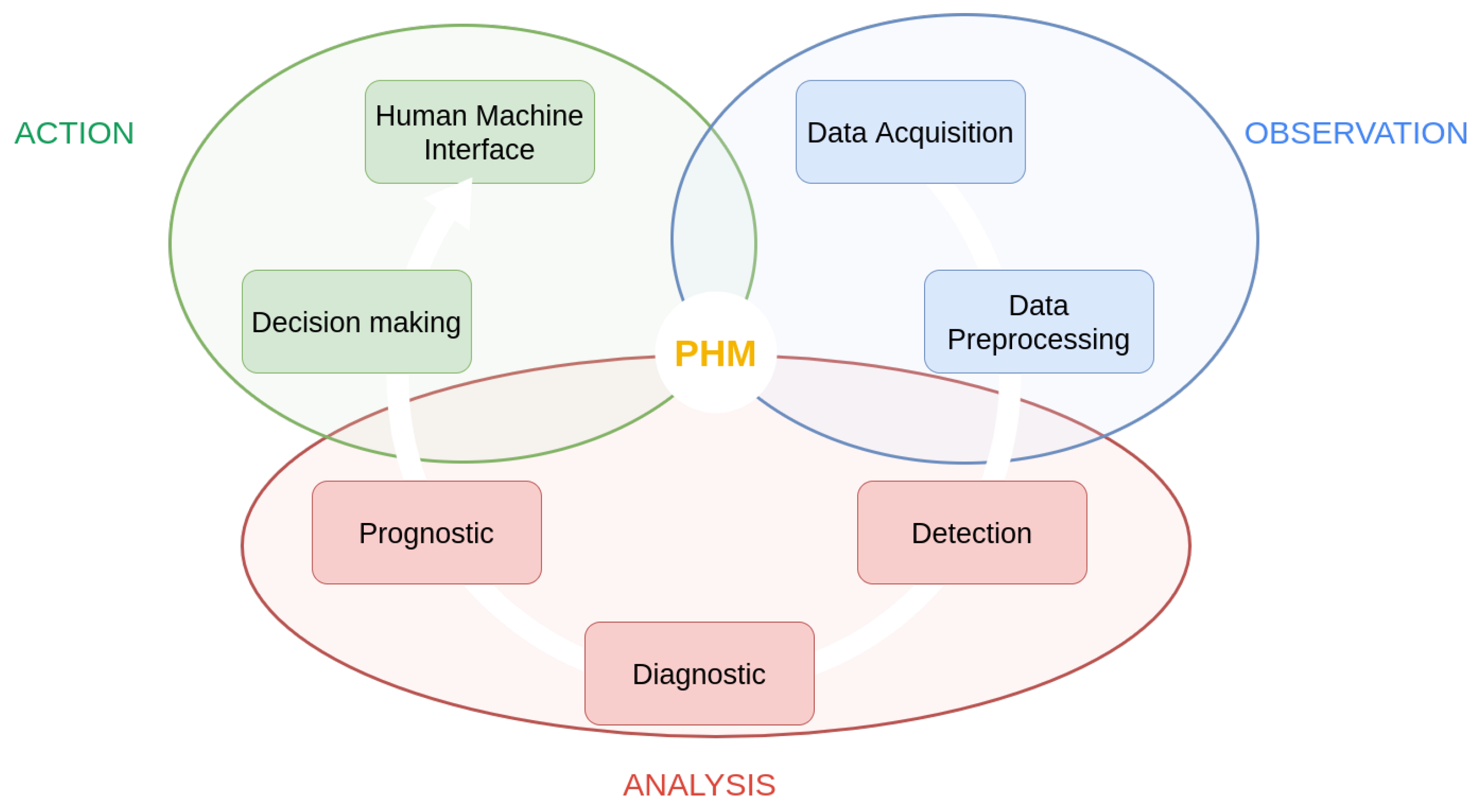
Electric actuation is one of the preferred research areas in the industrial sector to create more environmentally friendly aviation. As an integral part of the more electric aircraft, electromechanical actuators have several advantages compared to their pneumatic or hydraulic counterparts. First and foremost, they are lighter than conventional systems, which reduces the overall weight of the aircraft and, consequently, results in fuel savings. In addition to weight savings, these systems have a more compact design, allowing for greater power density within the same volume. Furthermore, unlike hydraulic systems, electromechanical systems do not require compression fluids by nature. These fluids must maintain their properties over wide temperature ranges and have a high ignition temperature, as in the case of Skydrol. These properties are difficult to find in nature, and the synthetic compounds used in hydraulic systems can be corrosive and hazardous to humans and the environment. By eliminating the need for these fluids, electric actuators contribute to the creation of more environmentally friendly systems and simplified maintenance procedures for airlines. Moreover, when integrated into the aircraft’s electrical harness, this actuation is conducive to implementing sensors and monitoring circuits. However, electromechanical systems are susceptible to potential issues not encountered in current pneumatic or hydraulic systems, particularly issues related to jamming. For a primary (or secondary) flight control actuator, this dreaded event must be avoided at all costs. Therefore, it is necessary to establish monitoring strategies to address the potential occurrence of these defects. These monitoring strategies are part of the overall Prognostics and Health Management (PHM) context; see Figure 1. Our work is part of the prognosis approach.

Figure 1.
PHM process, as defined in [1], Figure 1.
1.2. General Framework
To successfully diagnose and forecast the health of an actuator with a small amount of data, we have developed a method based on time series alignment. Let us sketch the contours of this type of method to explain how it can perform both the diagnosis and the prognosis step in this set of methods of PHM; see Figure 1.
In the workflow presented in Figure 2, firstly, the pattern vector is computed along time to build the time series of a learning database (known states). The second step uses the same pattern vector to monitor unknown states. The time alignment allows for comparing the time series corresponding to the actual operation with the time series stored in the learning database and with different time scales. This comparison allows for the computation of the Remaining Useful Life (RUL), its uncertainty, and an estimation of the current state of health.
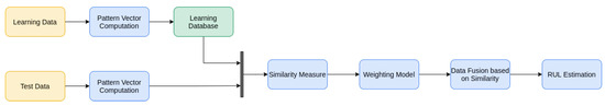
Figure 2.
Schematic diagram for all Trajectory Similarity-Based Prediction (TBSP) methods.
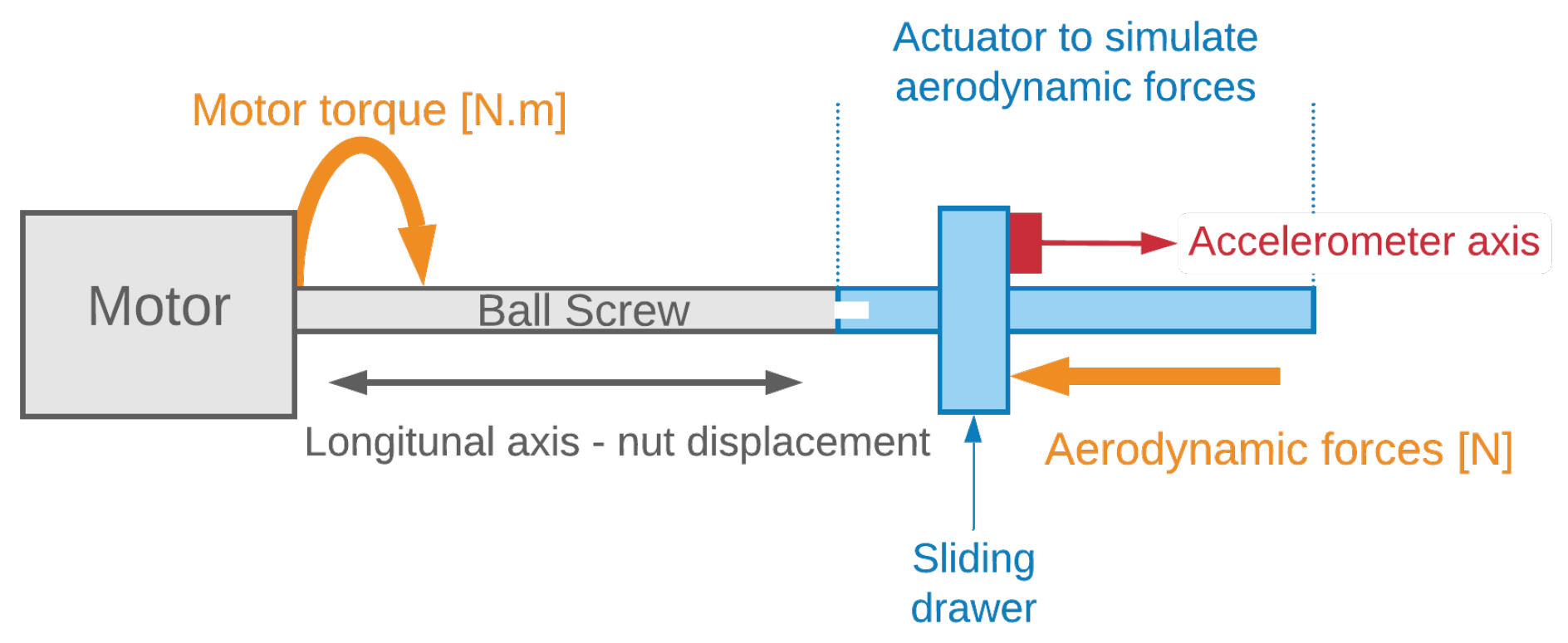
This work will be applied to compute the RUL of a ball screw actuator used for flight control, as shown in Figure 3, from vibration signals taken during its use.
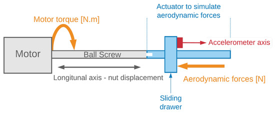
Figure 3.
Ball screw actuator instrumented on test bench, from [2]. Reprinted/adapted with permission from [2]. 2021, Eid.
1.3. Structure of the Paper
In our paper, we provide an overview of the temporal alignment methods used in the state-of-the-art in Section 2, which forms the basis of our approach. We then delve into the concept of time series alignment in Section 3, followed by a description of the necessary data pre-processing to create time series in Section 4. We explain the theoretical basis of alignment and improvements over the existing algorithm in Section 5. To evaluate the time series classification, we introduce a cost function in Section 6. By assessing the alignment of several time series, we can select a set of best candidates from the database in Section 7. Finally, we present a method to evaluate the uncertainty related to these alignments in Section 8.
2. State-Of-The-Art of the Prognostic Methods with Time Series Alignment
Aligning time series data involves putting in relation each component of the pattern vector, i.e., each relevant sensitive parameter, between source data (unknown ones) and those recorded in a learning database (structured set of available data). This alignment is based on minimizing a criterion measuring the distance between these series. Extrapolating data based on time series alignment requires the alignment of source data and a database of past recorded behaviors. This type of method is known as TBSP in the literature. Considering a database with the expected behaviors of the data that we wish to extrapolate, such as run-to-failure time series, this procedure needs less information than the deep neural network counterparts to obtain a relevant result. The idea is to compare test time series with the data in the learning database with a similarity measure. The most used similarity criterion in the state-of-the-art is the Euclidean distance and its variants. Then, the most similar candidates to the test data are fused. The latter model is chosen depending on the nature of the wanted output, an actual time instant, or the extrapolation of test data.
Dynamic Time Warping (DTW) was introduced by [3] as an algorithm to realize time series alignment, with many variants being realized afterwards. Other methods are also used for curve registration, such as the warplet approach of [4]. The first mention of a similarity-based method for RUL prediction was made by [5] to adapt it to the Commercial Modular Aero-Propulsion System Simulation (CMAPSS) [6] data set.
Later, [7] described a detailed framework applied to weld joint monitoring, namely the Ball Grid Array (BGA), in vibrating environments, or on a stochastic model of simulated data [8] as Similarity-Based Residual Life Prediction (SBRLP). The advantages of such an approach are numerous. It allows the realization of a prognosis with little available data, which is often the case in an industrial environment. Moreover, we can enrich the comparison database as the product’s life cycle progresses. Thus, without changing the method, the determination of the RUL will be all the more precise. However, if the database is not rich enough, the predictions will be subject to high uncertainty; this is the major drawback of the method.
The literature on predicting RUL from similarity measures or time series alignment uses data processing only or hybrid methods. The most widely used data set in the literature is the data set CMAPSS created by [6], composed of multivariate signals representing the degradation of a simulated jet engine.
For our part, we have chosen to validate our approach on data closer to an industrial application, from an aging bench of roller screw actuators, in the context of an aeronautical application.
The advantage of a standard data set is that it can provide comparable results between the work of different research teams. However, the massive use of CMAPSS [6] testifies to the recurrent problem of the lack of usable industrial data in PHM. Indeed, the few industrial data sets used are confidential, so the reproducibility of results between studies is not guaranteed. However, despite its demonstrated quality, the CMAPSS [6] academic data set only covers the analysis of several realizations of a single system in aeronautics. To overcome this, Refs. [8,9,10] use simulated stochastic models representing the degradation trend—anonymized vibration signals from an industrial data set.
3. General Description of Time Series Alignment
In the previous steps, we have created a database filled with time series. These data originated from accelerating aging scenarios where the monitored system cycled in a harsh environment. Thus, we can hypothesize that this database is filled with probable behaviors for the monitored system. A prognostic method consists of extrapolating the behavior of a system (we consider that the system behavior is characterized by its measurements) and diagnosing these extrapolations to estimate the monitored system’s future State of Health (SOH). In other words, two steps are realized: performing a regression and classifying the new measurement. To do this, because we consider the database filled with behaviors until the asset’s end of life, the extrapolation can be estimated by aligning the new time series (i.e., the new measurement, measurement on a new asset of the same family, the new features) to every one of their counterparts in . The extrapolated behavior will be the behavior of the best candidate for the alignment method. Furthermore, because the feature database SOH is known for every point, the new measurements can inherit the diagnostic labels of the best-aligned candidate of .
Thus, we develop a prognostic method based on time series alignment, i.e., finding a function that associates one point from one series with the other. The studied data are then divided into two ensembles:
- Points of the series to align from, called source points;
- Points of the series to align to, called target points.
In practice, let be a time series of length called the source and a time series of length called the target. In the latter section, we consider that and note (resp. ) the ensemble of indices of X (resp. Y).
The alignment can be framed as an optimization problem in which is found by minimizing an objective function . This injective function associates with every index of each point of X its associated index in Y. Hence, the association represented by can be incomplete because every point in Y is not necessarily associated with every point of X. In this PHM framework, we consider the source to have fewer points than the target. Even if this hypothesis is mandatory in our prognostic framework, the time series alignment method is independent of the length of each series. If this hypothesis is unverified, we can increase the sampling of either the source or the target.
More precisely, for our study, the vibratory signals captured on actuators, which are supposed to be independent, are extracted statistical descriptors of m points. These signals form a database noted as . The subscripts (or m), , and are introduced to realize a consistent notation scheme in the following sections. For this work, an actuator will be selected to simulate a set of data that would have been captured in operational use. Thus, these data will be contained in a matrix that will have to be compared to the data contained in a tensor . It is possible to determine the State of Health of the actuator from which the unknown signals come by comparing them to those in a database. This database can come from accelerated tests in a given environment or real operating profiles recorded in flight. The source series X previously defined will then be a column indexed by j, and thus a descriptor of the matrix . Hence, . The target will be noted as . This work aims to align the tested unknown series on the set of series . In other words, a descriptor will be aligned to the same descriptor of each actuator. The idea is then to arrange the candidates by order of similarity to . To do so, a cost function is defined to associate with each assignment function a real value. An information fusion step for each classified parameter is then performed to estimate the consumed lifetime and give a distribution representative of its quality.
4. Data Framework Surrounding the Prognostic Method
One monitored industrial asset’s RUL is estimated by comparing its operational behavior to a knowledge database. In general, this knowledge database contains a variety of realizations of similar assets in an industrial context. It could be either normal or degraded behaviors. It can also be filled with specific aging scenarios where the asset is accelerated to the limits. For the latter, in practice, the asset is placed inside an abusive environment, and we enable it to fulfill its function in a looping manner to simulate an accelerated aging pattern. We focus our work on the latter database content. Such a database is filled with time series representing physical measurements taken during the aging process of the same family of assets. We can model this database as a four-dimensional tensor with , where n is the number of acquisitions made per monitored system, p is the number of different types of measurements (current, voltage, etc.), q is the number of assets monitored (always of the same family), and r represents the number of points of acquisition. Note that the hypothesis is made that the data along all the assets share the same number of points r. Hence, they are only one shared acquisition profile repeated for every measure.
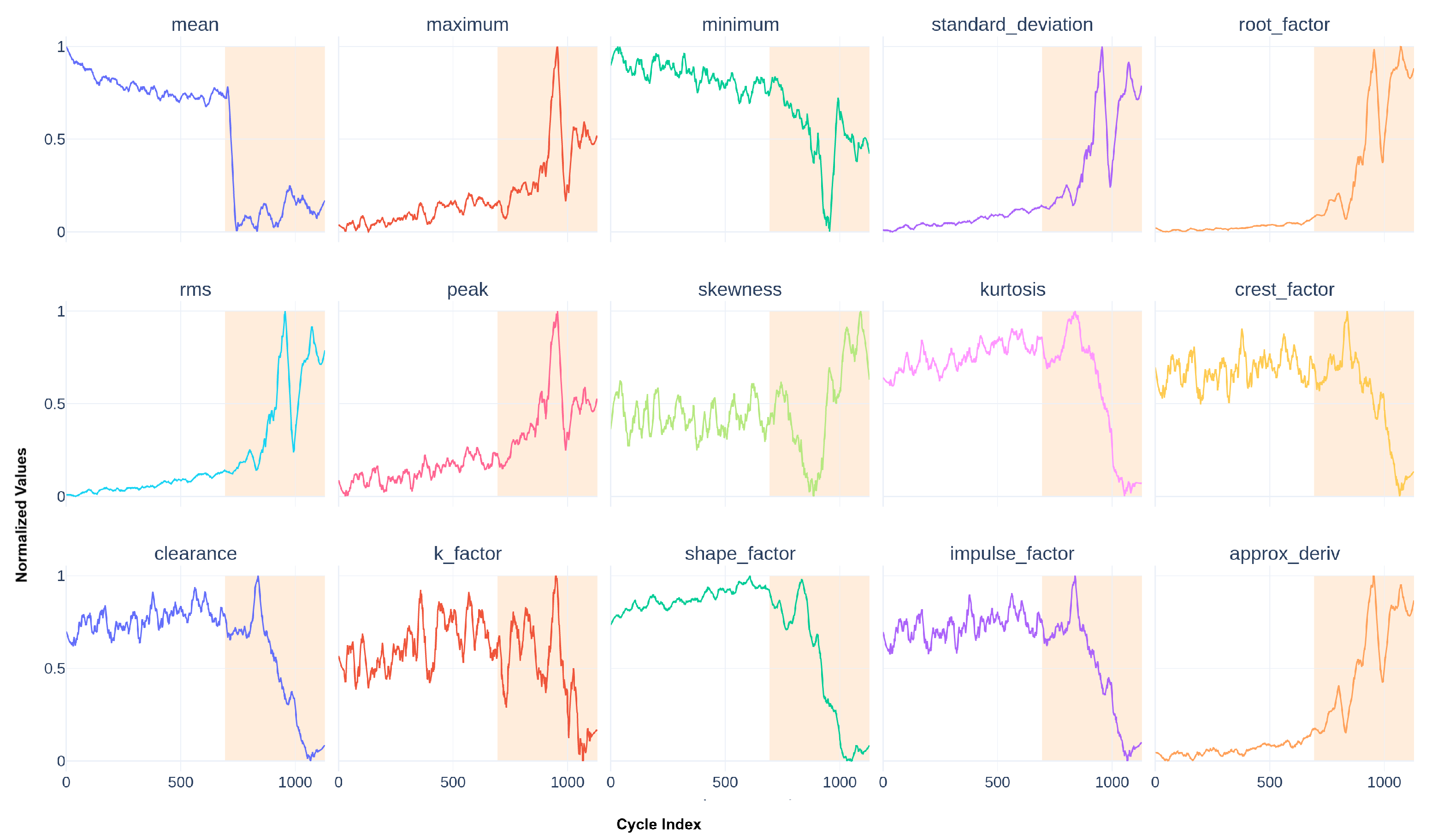
Instead of working directly with raw data measured from the monitored system, we provide several aggregation functions for each signal. One such function will compute a feature (or a descriptor). Let be a raw time series extracted from ; one function f can be defined as , and f can be seen as an aggregation function transforming an input vector to a unique value. Transporting a whole group of raw data into another set is called feature extraction. In this study, we concentrate only on univariate time series; hence, the data processed can be extracted from . We then apply feature extraction to a specific signal of size r taken from . If we calculate only one descriptor for every acquisition for a particular asset, we can reduce the size of the database to . Our study calculates p different descriptors for every time series. Thus, by collapsing the unitary dimension of the tensor and adding a new p dimension for each feature, we produce the database . n represents the number of points for each time series (now a feature), p is the number of different descriptors calculated, and q remains the number of assets studied. Note that, in our study, with our subsystem expert knowledge, we select statistical features taken from an acceleration signal in m s−2. They are presented in Figure 4.

Figure 4.
Smoothed statistical descriptors for the used actuators.
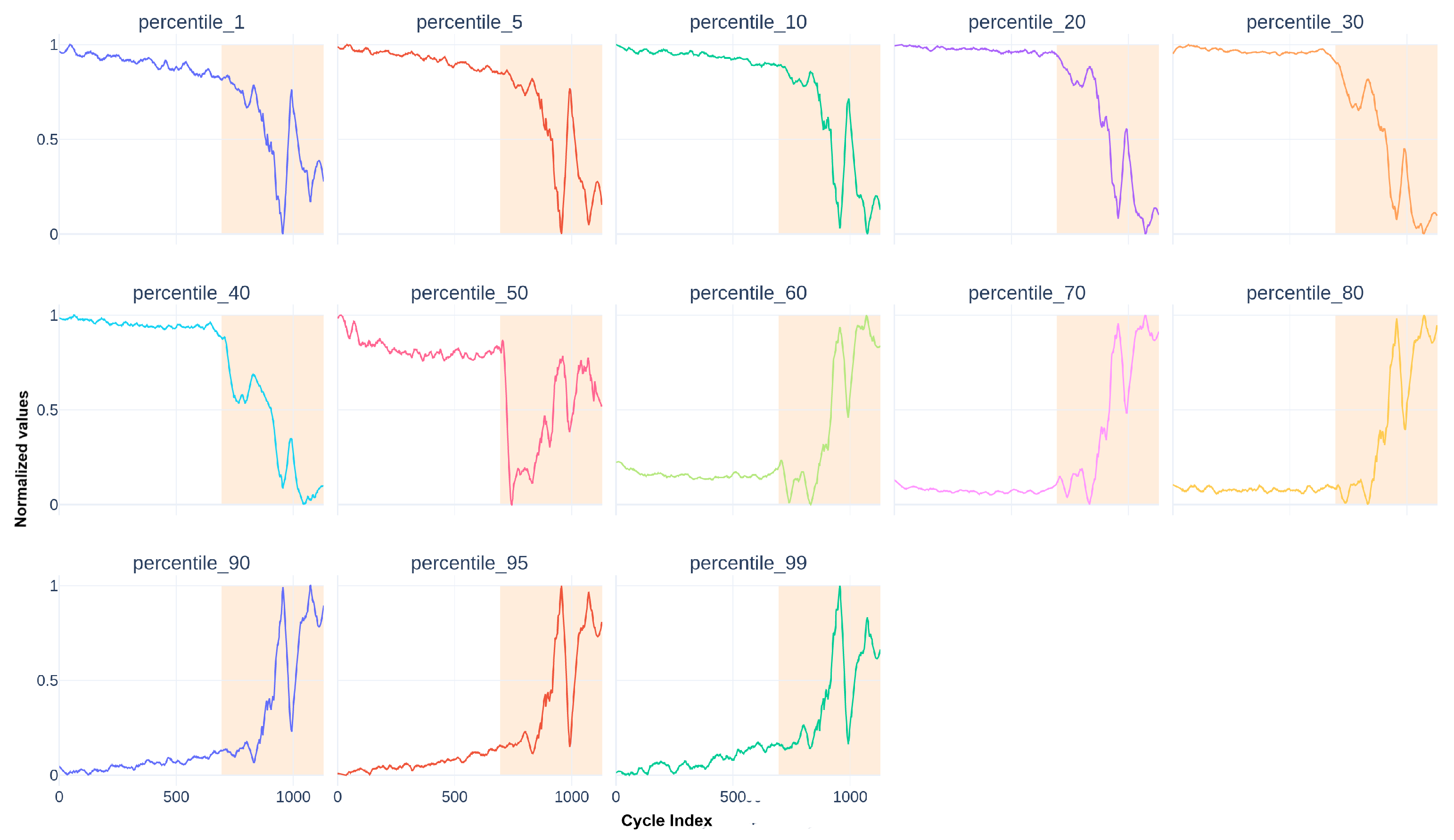
These descriptors are completed by percentiles of the actuator in deployment mode in Figure 5.
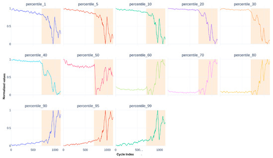
Figure 5.
Smoothed percentile descriptors for the used actuators.
Finally, we obtain features for each actuator.
In our application, we aged four identical actuators {Lower Right Actuator (LRA), Lower Left Actuator (LLA), Upper Right Actuator (URA), Upper Left Actuator (ULA)} by cycling them acceleratedly in harsh conditions, consisting of using the actuator at high frequencies through high and below-zero temperatures during an extended period of time. Three of them will be the reference actuators, and the fourth will be the actuator with an unknown state.
Let us note with a . To avoid notation overloading, let us define , which represents the same preceding feature whose values are indexed by the natural number in ascending order. This indexation could be superseded later by a series of timestamps, creating a new time series. At this stage, we have created an entire database of descriptors. We can use this information as input to our following prognostic model.
5. Alignment by Successive Displacements
After creating the database filled with reference curves, we need to define a similarity measure to allow the comparison with new data. We need to synchronize all the candidate time series to a reference and compute the distance between them. Hence, we use time series alignment (a principle also named time series registration). Let with and an unknown time series called the source and with a time series called the target. In our framework, we hypothesize that , and, if not, one can use interpolation methods to supersample Y. The goal of the time series alignment method is to find an injective function that associates with each index of points of X its corresponding neighbor in Y, thus characterizing the alignment. Note that all points of Y do not need to be associated with all points of X. All of this provides a natural time for rescaling.
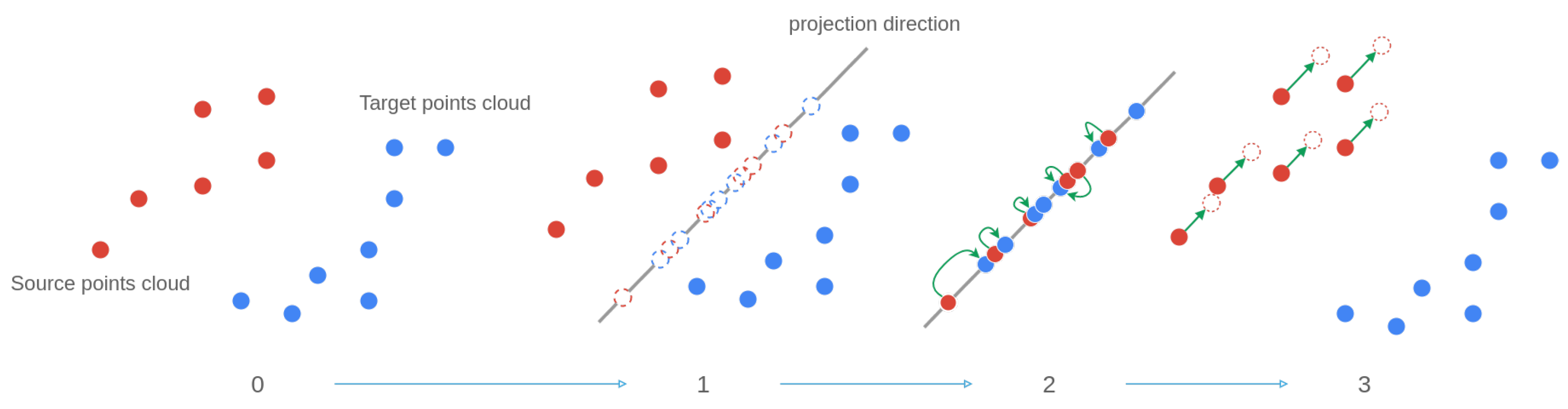
In state-of-the-art methods, the partial assignation of one time series to another can be considered as assigning the values of a 2-dimensional point cloud between one another. In this framework, time series values taken from can be considered a matrix with the time vector explicitly created. Thus, is the concatenation of and representing the time. For simplicity, timestamps can be replaced by integer indexes in ascending order. By doing so, we only keep the precedence relationship between each point. The time series alignment problem can then be reframed as an association problem between two point clouds with a heterogeneous number of points. This problem was studied by [11] with point clouds of several dimensions. The method called Sliced Partial Optimal Transport (SPOT) [11] was originally applied to histograms to transfer the color space of one image to another. The algorithm principle is illustrated in Figure 6.
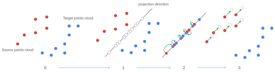
Figure 6.
Illustration of the principle of SPOT—initial method.
The first step of Figure 6 represents all the point clouds (i.e., times series). Note that, in our framework, we wish to align the data coming from the same descriptor between each other. Hence, we wish to align (in red in Figure 6) with (in blue in Figure 6) with . In other words, we wish to align the same features between different actuators.
In the second step of the method, the two point clouds are projected along one direction chosen randomly. We can note them, respectively, as . In the third step, an injective association between the points of and is computed: the assignation function .
Finally, at the last step, [11] solves an optimal transport equation to determine a uniform amount of movement to apply to every point of . Note that this movement is done in the dimensional space, along the projection direction chosen at step 1 of Figure 6 (represented by the green vectors in Figure 6).
Tested with the data at hand, our implementation of the method of [11] did not have relevant registration results. For example, the temporal ordering of each point was modified during the advection of the source to the target , which is problematic when trying to estimate a RUL with the time series processed. This is why we modified the SPOT [11] behavior to adapt this method to time series.
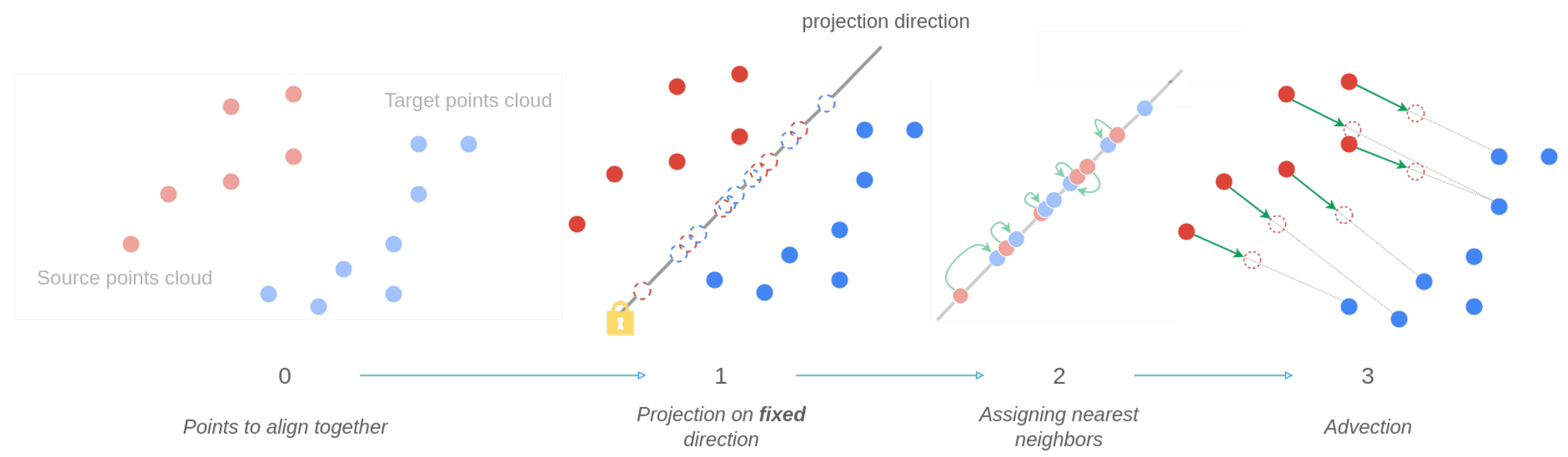
In Figure 7, the second and fourth steps of the original method are modified. Instead of choosing a random direction to project each cloud point onto, every point is projected onto an “optimal” direction in the sense that it minimizes a specific cost function in step 1. Moreover, contrary to moving in the same direction, source points now move directly towards each of their neighbors in the target cloud point. During this last step, the displacement quantity is not computed in the one-dimensional projection space but directly in the final two-dimensional space. In doing so, calculating discrete movement amounts in Euclidean space has replaced optimal transport equation solving. Note that, for step 2, we still use the original nearest neighbor algorithm search developed by [11].
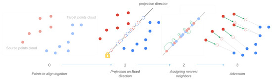
Figure 7.
Illustration of the modified time series alignment method.
Let us look at the detailed method.
- Step 1—Research for optimal projection space
This step consists of choosing the projection directions to solve the problem of nearest neighbor assignment in a 1-dimensional space. Let be the set of projection directions. This set is a sampling of the unit sphere of directions , with d being the number of dimensions of the problem. For any dimension considered, particularly for our 2-dimensional space of interest for time series alignment, comprises lines. In the work of [11], was a random sampling of . This randomness did not suit our needs. Indeed, the signals studied have specific dynamics that the projection step sometimes causes to disappear when projecting in a specific direction.
The assignment of the nearest neighbors in step 2 was carried out with signals with behaviors too far from the original signals before projection. As a result, the final alignment was not relevant. Therefore, it is necessary to find a set containing a set of lines providing a good final alignment result. The alignment method being iterative, a direction is assigned for each iteration. This is why the set consisting of several directions must be the solution minimizing a quality criterion.
This quality criterion will be the cost function , a variant of the cost function constructed further in Section 6. This optimization problem is formalized in Equation (1).
In Equation (1), represents the optimal set of directions determined for descriptor j and actuator h. The set is obtained by minimizing the sum of the movement costs, in one dimension, of the different states of the source cloud at each iteration. gathers these movement costs. For the first iteration, , ; for the second iteration, , ; and for the last iteration, K. The set on which the cost function is calculated is therefore of size K. Since no simple theoretical solution can be found for Equation (1), the set will be determined by an iterative optimization procedure. The principle is to sample the domain of definition of the set to find the optimal candidate about Equation (1). Note that the optimization result is not a single direction but rather a set of directions associated with each iteration of the alignment method; hence, . In total, there are directions to be found to perform the alignment on the database. The underlying idea is that the movement of the source cloud modifies its shape, and the previously chosen projection direction may no longer be optimal. The same cost function is used for each iteration. To enhance the computational efficiency, the calculation of projection directions is limited to two directions, where and . Importantly, these projection directions remain constant throughout the iterations of the method, and any changes in direction are contingent upon a condition evaluation based on the current alignment status. Specifically, the direction is employed while the source experiences significant movement. As soon as this movement subsides, the direction is selected to prevent the source from converging prematurely to a local minimum. This strategic decision significantly reduces the number of projection directions required.
Consequently, the source series is aligned with the target series using these projection directions. Upon achieving a specified cost threshold, the projection direction is transitioned from to , and the alignment procedure proceeds.
- Step 2—The assignation function source–target
This step involves finding the assignment function , recalculated at each iteration k, from the assignment of the nearest neighbors in the projected space between the points of the source cloud and the points of the target cloud . To do this, [11] developed an algorithm to solve the complete alignment problem in quadratic time, i.e., . Algorithm A1 (all the algorithms developed in this article are present in Appendix A section) allows for this quadratic assignment and represents step 2 of Figure 7. It can be divided into three main parts, with the first part, lines 2 to 15, allowing for constructing the first version of the assignment function . The second part, lines 17 to 20, decomposes the initial interval into linear sub-intervals, and the third part solves the assignment problem on the previous sub-intervals. Figure 8 represents the table nnAssignArray in Algorithm A1, which is associated with the assignment function .
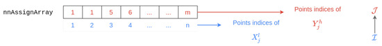
Figure 8.
Principle schematics of assignation function .
The assignment function is obtained by the Quadratic Assignment method of Algorithm A1 from [11]. The method then produces an assignment from the two clouds projected in a direction , the number n of points to align in the source, and the number m of points to align in the target. The sizes of the segments to be aligned are then stored in a structure param. Note that, in its current state, the segments to be aligned necessarily have n and m points, as the starting point index is automatically set to 1. However, extending the method to segments that do not start with the first point in the series is possible. For example, to align a 900-point segment with a 1130-point segment, the structure will be initialized as follows: param in Algorithm A1. After this initialization, the first nearest neighbor assignment is made by the Nearest Neighbor Match function defined by Algorithm A2. During this first procedure, different points in the source can be assigned to the same point in the target. These repetitions are then counted and stored in the nonInjMatch variable declared on line 5 and updated on line 9 of Algorithm A1. This information allows for the series to be decomposed into intervals and thus reduces the size of the interval considered for alignment. To this effect, the Reduce Range function described by Figure 2 of [11] is used. These new intervals created and representing a bijective assignment function must then go through the application of the Nearest Neighbor Match function in Algorithm A2, at line 17. After this second assignment, the intervals are decomposed into a set of sub-intervals by the Linear Time Decomposition function described by [11], Algorithm 2. This operation represents the third decomposition of a series into distinct intervals. A list of structures containing the start and end of each interval is then stored in the paramListArray variable. On each of these intervals, the nearest neighbor assignment is calculated at line 23, and then the Handle Simple Case function, which replicates the behavior described in Section 3.2 of [11], allows for certain configurations to be solved in linear time. Finally, after one final sequence of procedures, the Simple Solve function described by [11], Algorithm 1, allows for the final assignment to be obtained. Therefore, the function has been generated.
Algorithms A1 and A2 allow us to obtain, for an iteration, the assignment function . Step 2 of Figure 6 is then completed. This function will then be used in the advection model of the final step, step 3.
- Step 3—Advection model
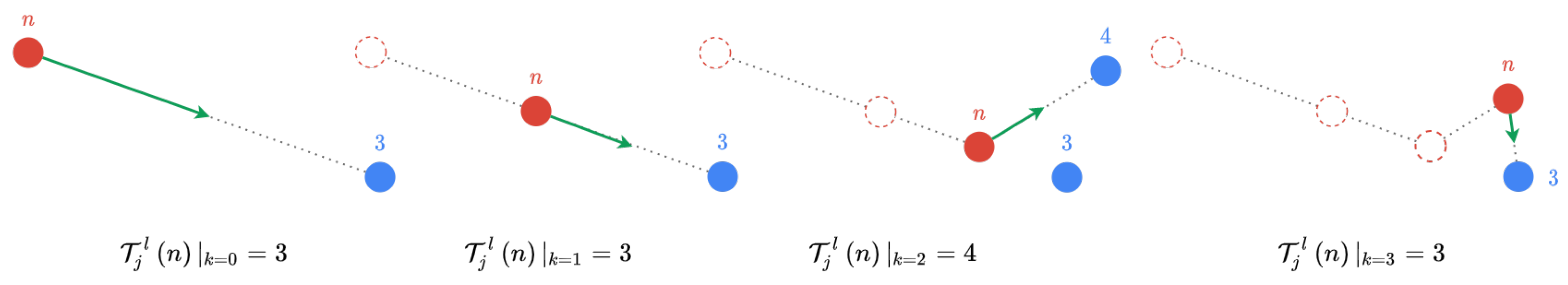
As schematized in Figure 7, the advection model developed differs from the SPOT method in [11], where the source points move towards their neighbors in the target by an amount calculated by solving a one-dimensional transportation problem. Here, a displacement amount is also calculated for each source point, but the points will then move by a given amount in the direction created between them and their respective closest neighbors in the target. Figure 9 illustrates this principle for a source point moving towards two different target points defined as its nth closest neighbor for each iteration. In Figure 9, the dotted red circles represent the positions of the source point before the current iteration.
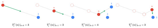
Figure 9.
Displacement example of the nth source point towards its affected neighbor (the third point) located in the target point cloud for 4 iterations.
The function in Figure 9 is the assignment function evaluated at the nth source point for the first iteration of the alignment of the jth descriptor of actuator l. At each new iteration of the transportation algorithm, the source cloud will move closer to the target cloud until it ultimately reaches it. In Figure 9, the displacement vectors of the source points are represented by a green arrow. Let be the source point considered at iteration k and be the target point corresponding to its closest neighbor at iteration k. Then, for each point, n and m, the displacement vector has a direction along the line passing through and is directed towards and has a norm, or movement quantity, equal to half of the Euclidean distance between and . Thus, the movement quantity (represented by the norm of the green arrow) is calculated using the dichotomy in Figure 9 to simplify the illustration of the concept. The movement quantity of the ith source point at iteration k with Euclidean distance is given by Equation (2).
In the case of the method developed in Algorithm A3, the movement quantity is calculated by dividing the remaining distance between and by a factor . Let d be the distance traveled by a source point. At each iteration, k, a distance can be associated with a point. The sequence of distances is then created. As a result, it is a geometric sequence with a ratio . Its partial sum thus has a simple expression,
which converges, for an infinite number of iterations, , to the magnitude . The advection model, therefore, reaches a stability point. By extension, the alignment algorithm necessarily converges towards the target, but, as it stands, it is not yet possible to evaluate the quality of such convergence. A cost function will be developed in Section 6.
In more detail, the Advection function of Algorithm A3 produces a source cloud from the two clouds to align and . The assignment table nnAssignmentArray represents the function and sigmoid, an array containing the previous variable for each direction. Lines 2 to 4 initialize the structures to calculate the total distance traveled by the source cloud. Lines 6 to 9 define and , which represent the coordinates of the points to be reached in the target , while and represent the coordinates of the starting points in the source. The distance between these two points is then calculated on line 12. The displacement amounts and are calculated on lines 15 and 16 as a proportion of the distance between the source and the target. The coordinates of the source point cloud are then updated on lines 18 and 19. Finally, an advection cost is calculated as being the normalized sum of the distances traveled by each source point and the moved source cloud . Note here that the advection cost differs from the cost function developed in the following Section 6.
Now that all the steps of Figure 7 have been detailed, the global Algorithm A4 is developed to bring together all these functions and obtain the final alignment of a time series X with a series Y.
The Time Series Alignment function produces the shifted source point cloud using two point clouds and , the set of optimal directions found in Equation (1) , and an array of hyperparameters weightArray. The Time Series Alignment function then performs K iterations of steps 1, 2, and 3 in Figure 7 as long as the cumulative displacement of points from the source to the target is not zero. The variable cost is declared in line 7 with a non-zero value and updated in line 56 with the absolute value of a cost calculated by the function. The cost will be zero below a limit. This avoids the algorithm continuing to iterate when the displacement cost is of the order of machine precision and potentially a numerical error. Now that the automatic stopping criterion has been presented, let us discuss the operation of Algorithm A4. The first lines of Algorithm A4 initialize the variables, and line 6 preserves the initial values of the source point cloud . For reference, the latter is defined as , where the notation keeps only the , i.e., the initial time series , which is . The iterative loop then begins by testing, at line 8, if the calculated cost, which is different from the displacement cost of the cloud, is not negative. This is when the source cloud points converge very slowly to the target. Therefore, the projection direction index is modified to maintain an optimal convergence rate. Consequently, the points of the shifted source cloud will be projected onto the second and last direction of the set . As in Algorithm A1, a matrix projection onto a line is translated by matrix multiplication. Indeed, with and , the operation at line 22 creates a column vector stored in projSrcWIndex with its respective index vector. The same operation is performed in Algorithm A4 at line 26 for the target cloud. The arrays projSrcWIndex and projTargetWIndex are then sorted in ascending order of their values in the first column of these two structures. This step allows the projected points to be sorted while retaining their respective indices and, thus, their positions in the initial cloud. Two new column vectors projSrc and projTarget are created at lines 35 to 38 with the ordered points. The Quadratic Assignment function described in Algorithm A1 is then applied to these vectors to obtain the value of the assignment function via the nnAssignArray array. Afterward, manually determined hyperparameters are chosen to create two values of a sigmoid function. These two values will weigh the displacement on the two dimensions of the source cloud towards the target cloud. Ranging between 0 and 1, they allow the displacement of the source to be moderated to avoid excessively rapid convergence towards a suboptimal alignment. The Advection function of Algorithm A3 then produces the displaced cloud at line 49. The latter is added to the states of the source , and the local cost is updated. Repeating these steps until the null displacement of the source towards the target is achieved allows the time series X and Y of any size to be aligned.
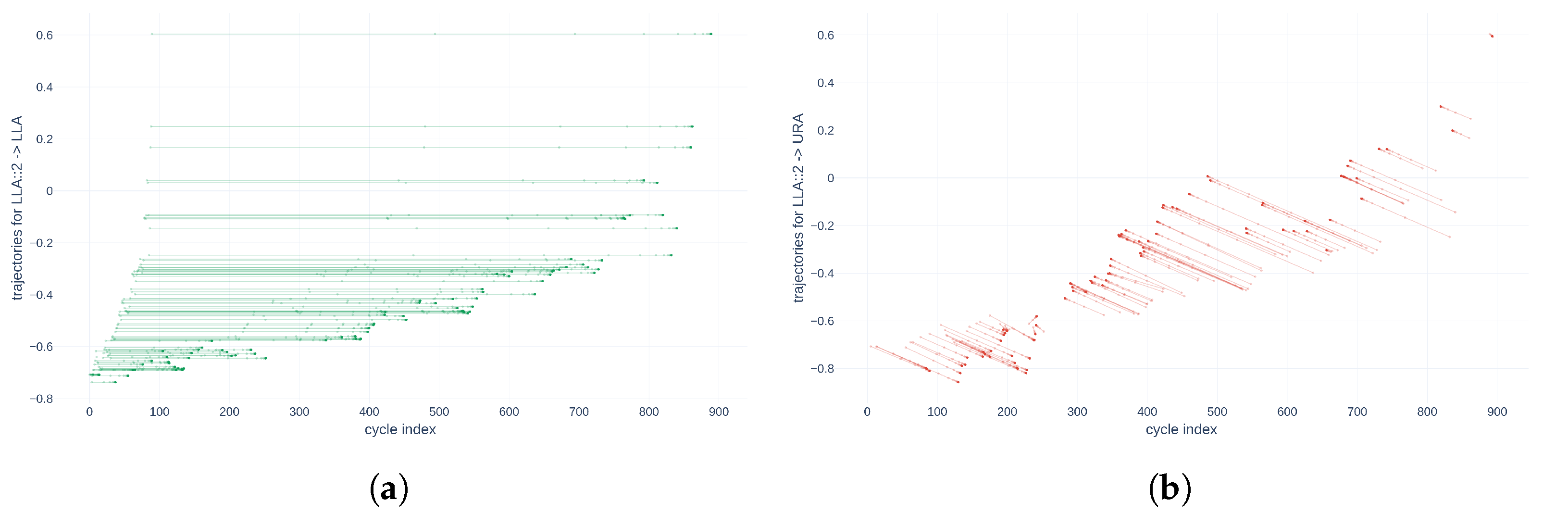
Now that the global time series alignment algorithm has been detailed, it is tested on experimental data. To do so, the source is represented by the Root Mean Square (RMS) descriptor of the LLA actuator, and the same RMS descriptor of the LRA actuator represents the target. The point clouds associated with each of them are denoted, respectively, as and . To demonstrate that the method works with series of all sizes, the source will be truncated to 900 cycles, and, from the resulting segment, of the points will be randomly selected to form . In contrast, the target of 1130 points will remain unchanged as . The alignment results are shown in Figure 10.
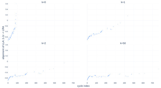
Figure 10.
Random alignment of 10% of selected points of the descriptor RMS of LLA towards the descriptor RMS of LRA.
Figure 10 represents 4 different states of the source point cloud during the alignment procedure: , , , and . The spacing of the iterations k is not constant, to better visualize the displacement of the source towards the target. Indeed, the displacement is more significant during the early iterations of the alignment algorithm. This result demonstrates that the method works even for incomplete series, as long as the number of points in the unknown source series is less than that of the known target series that constitute the database. However, at this stage, it is impossible to quantify the quality of such an alignment. This is why Section 6 details the development of a new cost function .
6. Quantification of Time Series Alignment
Each alignment procedure assigns a similarity metric to discern the most appropriate candidates within the database, as expounded upon in Section 3. The establishment of precise criteria to define a meaningful series alignment is paramount in this context. However, the complexity of our particular scenario is compounded by the inherent ambiguity of the data composing the operational series, denoted as . Consequently, when the alignment of with is successfully achieved, no baseline exists to compute the deviation from a known ground truth.
In response to this challenge, it becomes imperative to introduce an intrinsic quality metric represented by . This metric serves as a quantification that operates independently of prior knowledge concerning the data’s inherent characteristics. The incorporation of this methodological approach represents a crucial step in addressing a fundamental challenge inherent in our research endeavors.
Let us provide an overview of the method developed in Section 5. The objective is to align a time series, denoted as , with another time series, referred to as . The alignment process commences by transforming both time series into point clouds, resulting in and . These point clouds are subsequently projected onto a common set of directions, represented by . For a given direction, two new series, and , are derived, from which an injective assignment function is constructed. The values of this assignment function play a pivotal role in the advection model, generating point displacements from to . Since this displacement transpires within the confines of a two-dimensional space, the advection model calculates a displacement vector for each point within the source cloud, utilizing the canonical basis of . Let us denote this orthonormal basis as , with its constituent vectors represented as and .
The entire process, which includes the projection of the source cloud, construction of the assignment function, and subsequent point movement, is iteratively repeated a total of K times to achieve convergence between the source and target points. This comprehensive methodology represents a critical step in our research and contributes significantly to the academic discourse in this domain.
Within the framework of this method, a crucial step involves extracting pertinent information to assess the quality of an alignment. To shed light on this aspect, we examine the behavior of the assignment function denoted as , and its characteristics are visually represented in Figure 8. This function establishes associations between each element in the source and its corresponding counterpart in the target. In the context of an alignment procedure spanning over K iterations, we introduce the matrix , which aggregates the values of the function computed at each iteration. Mathematically, this matrix is expressed as . This analytical approach is pivotal in our methodology, as it facilitates a deeper understanding of the alignment quality assessment process. Let us further characterize such a function. is defined in with values in . Let be the column k representing the set of values taken by at a given iteration. If the source shares similarities with the target series, after detailing the alignment method in Section 5, it is reasonable to suppose that the images of the function should be almost identical between each iteration. On the other hand, a completely random alignment could result in wide variety among the image sets of each function . The image set of an assignment function is a repetition arrangement of n elements (the indices of the source points) in a set of m elements (the indices of the target points). There are then a total of possible image sets. In the matrix with K columns, there would still be different column combinations. Thus, if convergence from the source to the target does not occur for a completely random alignment, the columns of would all be different. In other words, for all . Conversely, in the limiting case where the alignment is perfectly consistent, all columns of would be identical. In other words, for .
According to the definition of the function , this would mean that the points of the source would all move, as the alignment progresses, towards the same points of the target . Thus, in the advection model, the direction of the displacement vector of each point in the source would remain constant as the iterations progress. This leads to the creation of Hypothesis 1.
Hypothesis 1.
In the case of a perfectly consistent alignment, a unique direction of movement is associated with each source point during the convergence process.
Hypothesis 1 alone is insufficient to establish a function capable of quantifying the quality of an alignment. This hypothesis, on its own, permits pathological alignment scenarios, such as the complete inversion of all points in when aligning it with . In this scenario, the first point would align with the last point , while the last point would align with the first point of . Such an alignment would inherently be considered suboptimal. Given the behavior of the advection model described in Algorithm A3 and the characteristic monotonicity of our descriptors in the ideal case, this particular alignment example would result in the substantial alteration of the initial value of the source cloud point. In other words, for a given point with an index i, during K iterations of the algorithm, .
Preventing such configurations necessitates constraining the angular variation in point directions within within the advection model. The limiting scenario, in this regard, implies exclusively horizontal movements. To formalize this, let represent the set of displacement vectors generated by the advection model at a specific iteration. For each point, an ideal displacement vector for the alignment, denoted as , can be derived as follows:
with being the usual scalar product defined on taking values in . This translates to the collinearity of the ideal vector with the base vector . Therefore, for the construction of , Hypothesis 2 must be added.
Hypothesis 2.
In the case of a good alignment, any motion vector with must be collinear with the first vector of the canonical basis , where denotes the usual scalar product defined on with values in .
Let us summarize the two previous objectives.
- Hypothesis 1 would force the function to converge towards a unique value.
- Hypothesis 2 would require the alignment to have little effect on the elements of the source . It would become the target to be reached during the alignment.
Lastly, given the iterative nature of the alignment method, constructing a cost function solely based on Hypotheses 1 and 2 would introduce bias linked to the number of iterations required for convergence. To elaborate, as the method’s stopping criterion is not contingent on the number of iterations, distinct alignments could be unfairly penalized based on their convergence speed. Notably, this criterion, centered on the convergence speed, falls outside the scope of this study, which emphasizes the estimated accuracy of the result rather than the method’s computational performance.
Consequently, this scenario paves the way for introducing a third and final hypothesis to shape . A large number of iterations would correspond to an extended path traversed by the source’s points. This scenario suggests that the source signal represents the non-uniform compression of the target signal . In accordance with Hypothesis 3, it has been determined that these dynamics should not factor into the penalty selection. This nuanced perspective ensures that the focus remains on the alignment’s outcome and associated accuracy while disregarding the intricacies of the method’s convergence dynamics.
Hypothesis 3.
The temporal dilations of signals are not penalized in the alignment method.
Now that the three fundamental Hypotheses, 1, 2, and 3, have been stated to determine the criteria to be taken into account in the cost function , let us focus on constructing the object on which it can be applied.
To do this, let us define , a matrix containing all the intermediate states of the second dimension of the source cloud during the alignment phase. Only the column of the source cloud containing the values is considered, given our desire not to penalize temporal dilations (see Hypothesis 3). In more detail, the source state matrix will be defined as in Equation (5).
The developed cost function will then be applied to the matrix and produce a positive real number. It is defined in Equation (6).
Hypotheses 1 and 2 are modeled by the term , which represents the sum of squared differences between the intermediate states of the series and its initial state. Hypothesis 3, on the other hand, is modeled by the normalization factor K, representing the number of iterations of the alignment algorithm present in the denominator of expression 6. Indeed, the more iterations that it takes to align the source to the target, the more the source series is dilated. By normalizing the expression in this way, this effect no longer impacts the value of the cost function. Finally, the sum over the iterations of the alignment algorithm aggregates all differences over the total number of iterations. As a reminder, for each iteration k, a function is calculated that assigns each source point to its neighbor in the target. The value of the function will likely change at each iteration. With the expression of given, evaluating it allows us to answer the different hypotheses made to quantify the value of an alignment. In the case where Hypotheses 1, 2, and 3 are met, the cost function defined in Equation (6) is zero. Indeed, , so . In the case where one of the hypotheses is not met, since is a double sum of squares, we have
A cost function is theoretically defined in Equation (6). Let us now test its relevance with experimental data. To do so, the source to be aligned will be the RMS descriptor of the LLA actuator and the target will be the same descriptor chosen from the set of actuators .
Our validations will always follow the same approach. The LLA descriptors will be taken as the source, and the corresponding descriptors of the other actuators will be taken as potential targets. Indeed, we assume a similar behavior exists in the database without being completely identical.
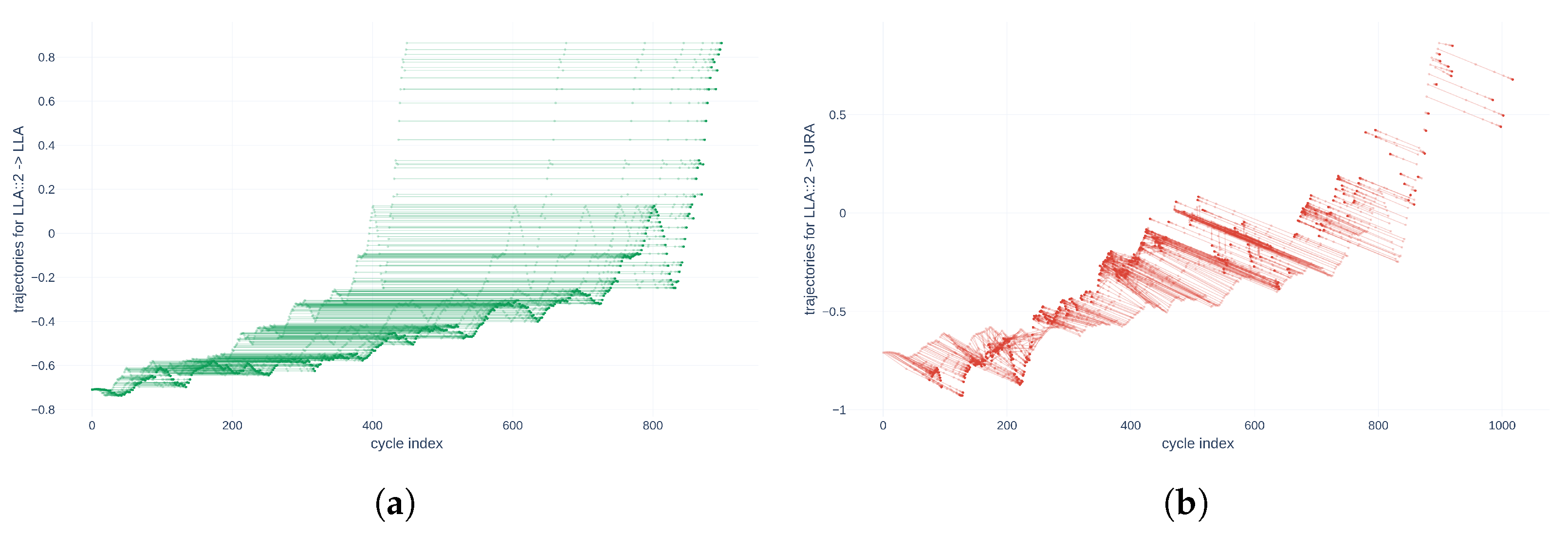
The data used in this work come from accelerated aging tests of various electromechanical actuators. The calculated descriptors share the same number of samples and sampling frequency. Let us simulate a source with a uniform compression factor relative to the targets to demonstrate the general nature of the cost function . Every other point is then selected in the source . Additionally, this same source is truncated to 900 points. A point cloud is then created using the method described in Section 5 to obtain . The resulting point cloud has 450 samples. This two-dimensional data series represents the behavior of an actuator descriptor evolving from 0 to 900 cycles. Thus, the goal of the alignment method is to align the last point of the source with, at a minimum, the 900th point of the uncompressed target . Figure 11 shows the trajectories of the source points as the alignment algorithm converges in two different configurations: an alignment of the compressed source on itself, uncompressed in Figure 11a, and an alignment of the compressed source on the descriptor of another actuator, uncompressed in Figure 11b.
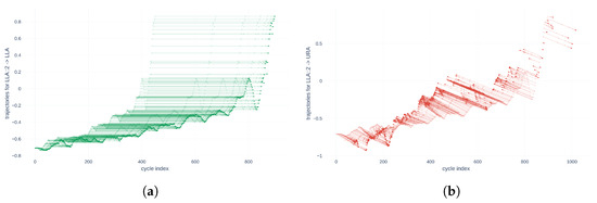
Figure 11.
Point trajectories for descriptor compressed by a factor 2 RMS of LLA on different target time series and associated cost function values. (a) Alignment Cost function value: ; (b) Alignment Cost function value: .
The two parts of Figure 11 illustrate very different behaviors. Indeed, Figure 11a represents the trajectories of source points that are all parallel. The last point of the compressed source reaches the 898th cycle during its alignment in the target, which differs by only two cycles from reality. On the other hand, Figure 11b represents more disparate trajectories of source points. In addition, the 448th point—in other words, the ante-penultimate aligned point—reaches the 1016th point in the target. This difference is explained by the fact that the target data differ from the source data, while the source is aligned with its homologous descriptor in the URA actuator. However, this information confirms the idea that, with this method, the quality of a series alignment can be quantified by the behavior of the movement directions of each point. Thus, the behavior of each point could be quantified by the function constructed in Equation (6). The cost values obtained from the two alignments then make it possible to verify the wanted behavior of . Thus, in Figure 11a, the function does not penalize the dilation of a series during alignment, and Hypothesis 1 is verified. Hypothesis 2 is also confirmed because the directions of each point are horizontal and therefore collinear with the first base vector , . Finally, Hypothesis 3 is validated because the value of the cost function is zero. For Figure 11b, since the three fundamental hypotheses of are not verified, the value of the cost function is a positive non-zero value: .
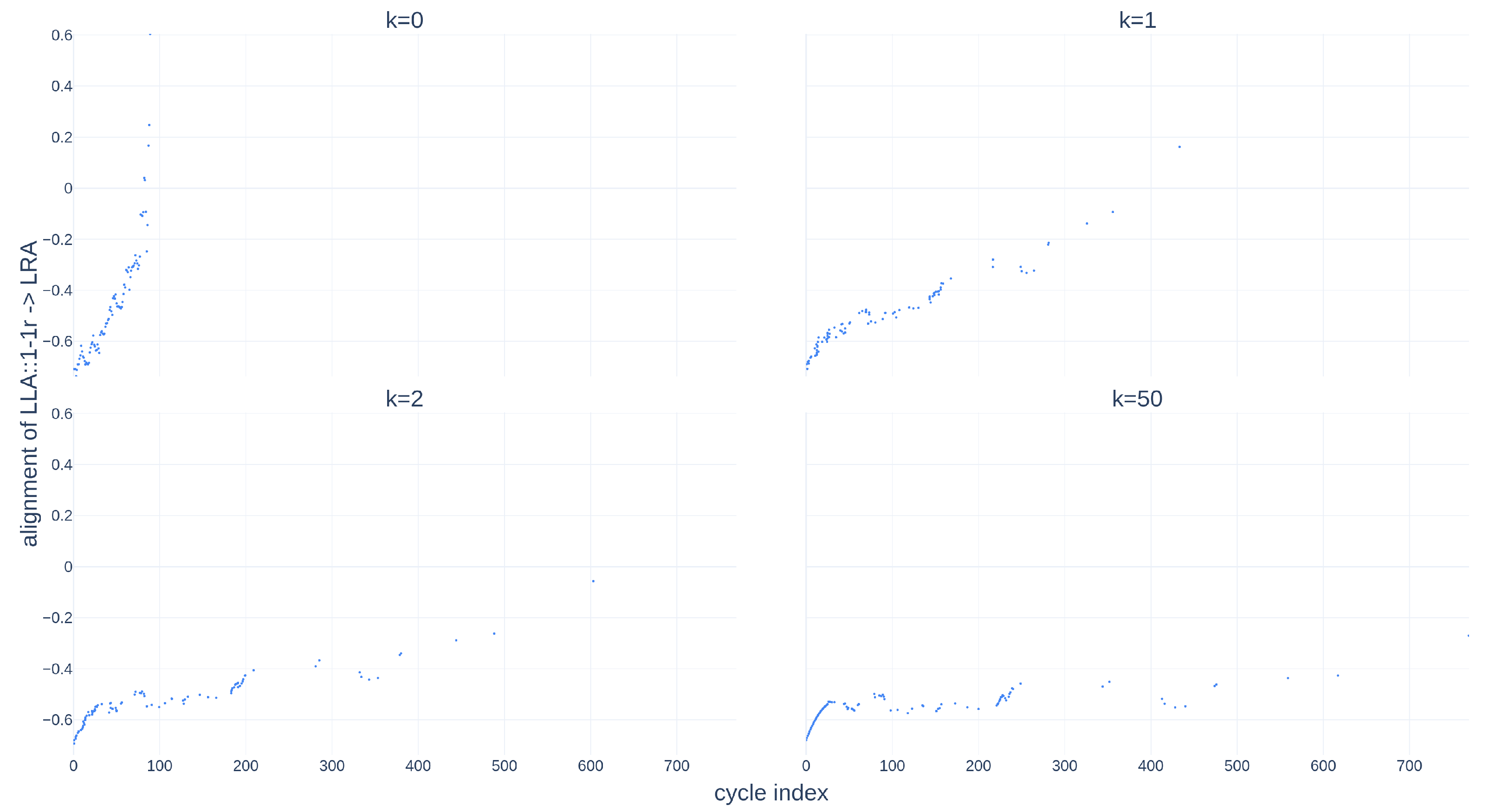
Previously tested with a constant compression factor, the time series alignment method developed here shows relevant results for non-uniform compression factors; the cost function allows us to quantify them. However, why focus on a non-uniform compression factor? This configuration could model a variation in the environmental conditions of using an actuator. In this case, the actuator would not age regularly, as represented by the data used here, namely with pseudo-exponential dynamics during 1130 cycles of constant use under invariant conditions. This is why a non-uniform compression factor remains an interesting study point. For this modeling, a point on n, with randomly drawn at each new selection step of the previous source , will be selected. By selecting only of the points from the source, the cloud is obtained. The experimental protocol is identical to the one used to obtain Figure 11. Figure 12 is then produced.
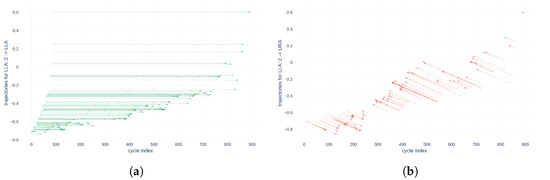
Figure 12.
Point trajectories for the alignment of the descriptor RMS of LLA with 10% of randomly selected points and the associated cost function values. (a) Alignment Cost function value: ; (b) Alignment Cost function value: .
Figure 11 and Figure 12 show that when a compressed or pruned descriptor of a given actuator is aligned with the original one, the cost function is null, whereas when it is aligned with the same descriptor of a different actuator, the cost function is non-null.
We construct a cost matrix for each descriptor. Then, we construct the sum of these matrices, , and obtain a cost matrix, shown in Figure 13.
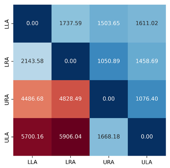
Figure 13.
sum of the cost matrices for the database . A divergent color scale is used with deep blue representing the lowest values and intense red representing the highest ones.
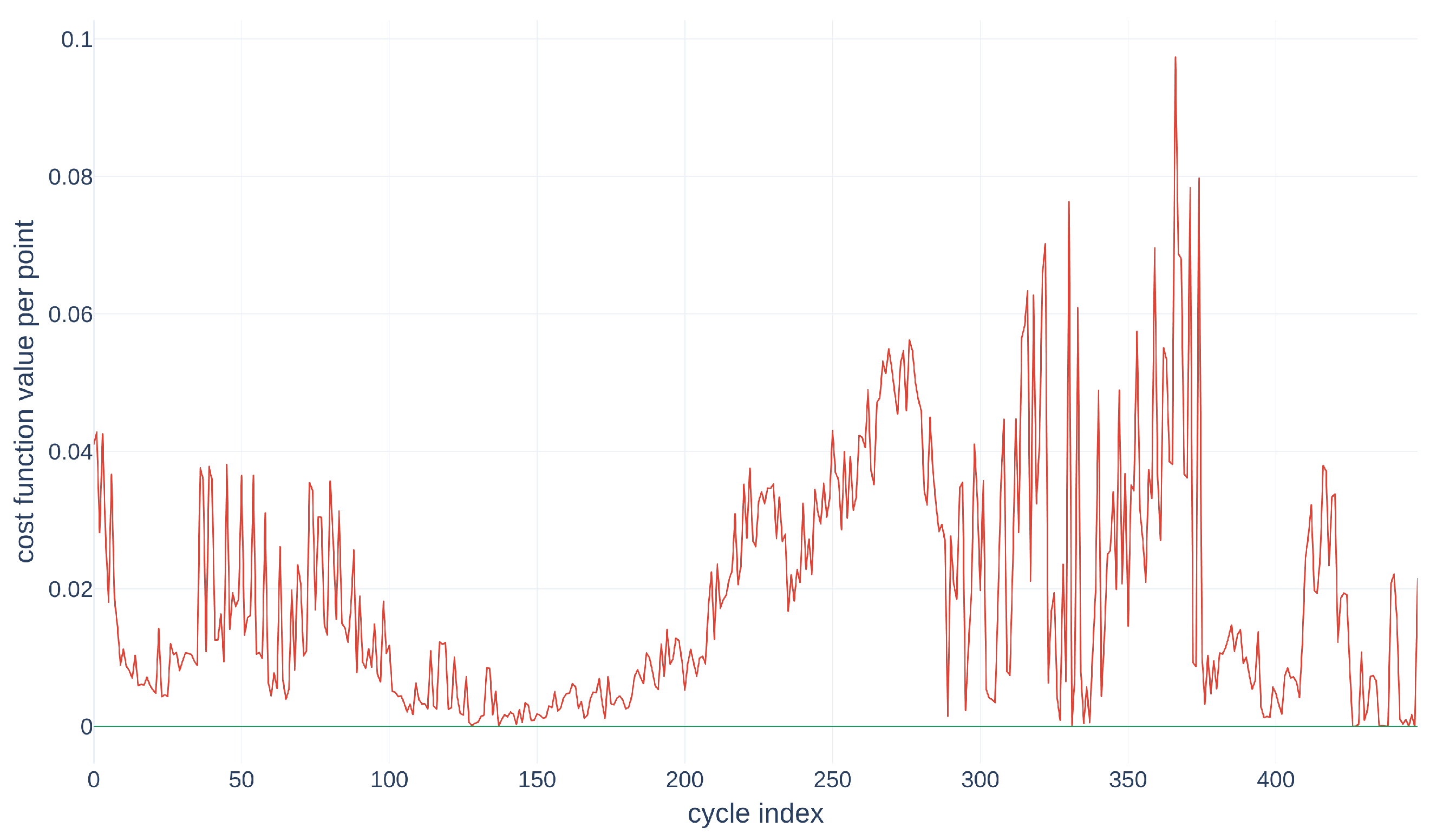
The function then allows us to attribute to a given alignment an actual value representative of its quality—in other words, representative of the similarity of a source time series to its target. It is then possible to change the scale to consider not the global quality of an alignment but the variation of each point of the source series from its initial state. This represents the penalty associated with each point in the alignment, which was aggregated by the function. This new term can be formalized by
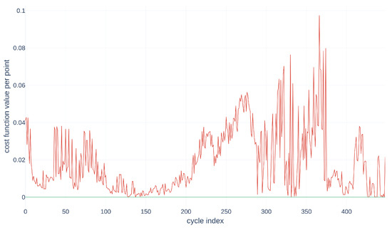
Figure 14.
Visualization of the variability of the trajectories according to the points for the alignment .
In Figure 14, the green curve represents the variation of for the alignment , and the red curve represents the variation of for the alignment . This figure helps to identify regions of low point movement—in other words, segments of the source curve that closely resemble the target curve, namely an initial region within points, a second one within , a third one within points, and the last one from the 376th point onwards. The second and last regions, with low values, coincide with the areas of low point movement in Figure 14. This information could then be integrated into the subsequent steps of the algorithm to enhance the quantification of uncertainty in the alignment method.
7. Selection of the Best Candidates in the Database
Each descriptor is aligned with the corresponding descriptors of each of the three actuators in the database. The alignment cost matrix in Figure 15 is then constructed, from which we extract the minima.
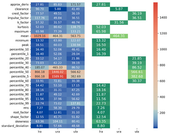
Figure 15.
Alignment cost matrix .
This allows us to determine the most representative actuator of the base. Each descriptor of the unknown actuator is associated with the most representative actuator in the database. It is then necessary to aggregate this information.
Thus, let us introduce the minimum cost vector :
contains all minimal evaluations of the cost function per descriptor alignment. In the case studied, the matrix has lines. becomes the basis from which the weights will be computed. In the first step, is normalized using the function
In expression (9), the function median used corresponds to the value of , which separates the matrix into two sets of equal cardinality. The interquartile range is defined between the first and third quartile Q. Therefore, ordering represents the deviation after eliminating the 25% lowest value elements and the 25% higher ones. Since Figure 15 highlights highly dispersed alignment costs, this normalization method is chosen to minimize the impact of outliers. Once this robust scaling is applied, the normalized exponential function is applied to the vector of weights calculated with Equation (9). This results in a vector whose sum of elements will be unitary. Thus, the vector of weights is obtained at Equation (10) from the vector .
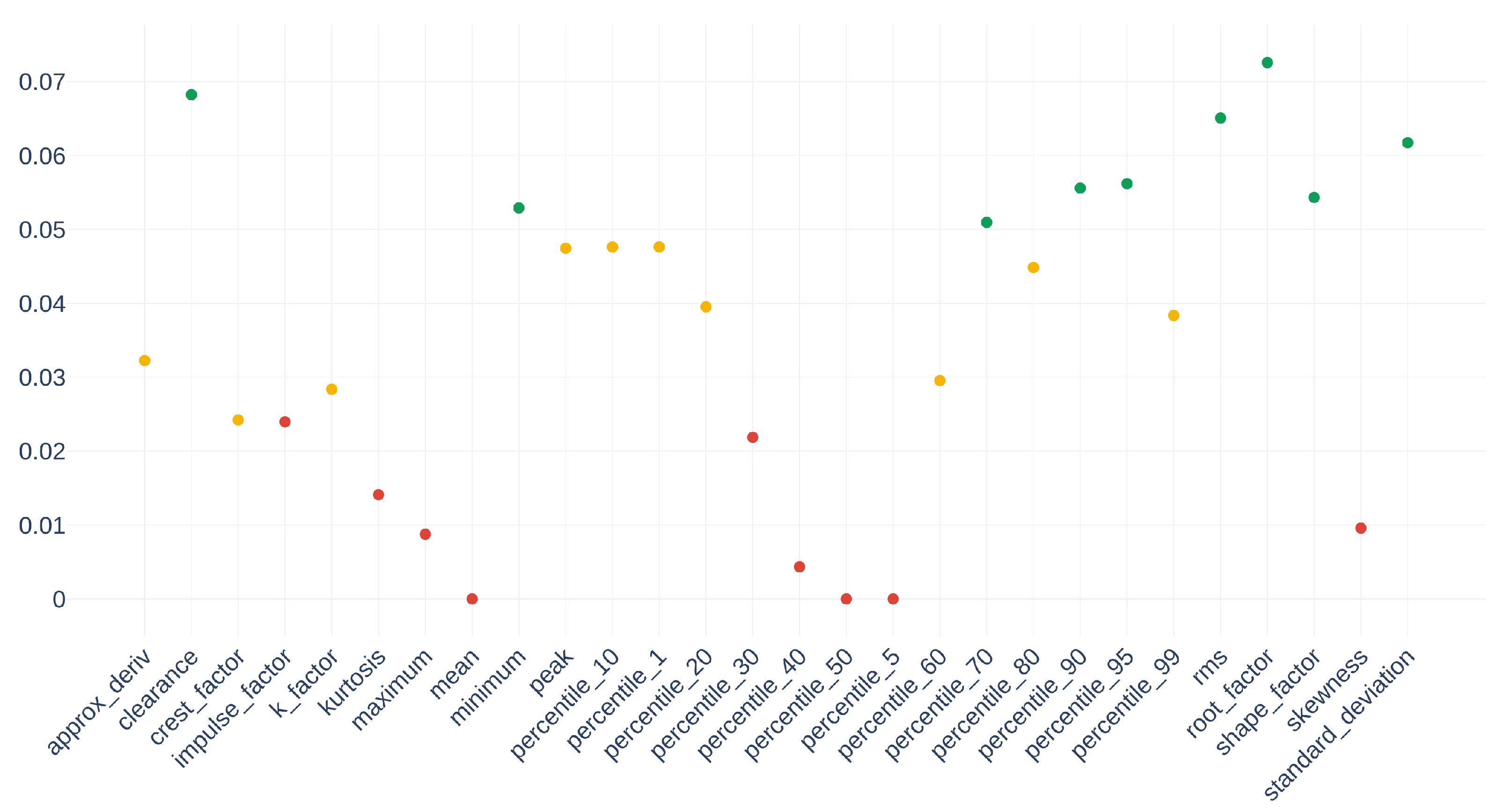
Figure 16 gives the normalized values of weights for all selected descriptors.
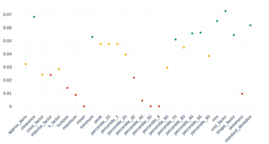
Figure 16.
Vector , normalized values of weights for all selected descriptors.
By crossing the information in Figure 15, it is possible to match their respective costs by the function , represented in Figure 16. Thus, they have an individual cost of , , and . Since the median of is , the values taken by the alignment quantization of these descriptors are 20, 25, and 16 times more significant than their neighbors in the optimal cost vector . Therefore, the weight determination scheme is consistent and represents the dispersion of the values well.
8. Uncertainty Measurement
The preceding sections have expounded upon the alignment procedure, which enables the identification of the most similar actuator within the database (with vibration signals here). For each time series associated with this actuator, we can determine the time index of the point aligned with the current point in the corresponding time series of the actuator under investigation. Consequently, for each parameter, the aforementioned index represents the consumed lifetime as a percentage. The subsequent phase entails amalgamating these distinct values and introducing a measure of uncertainty into the resulting composite. In the ensuing discussion, we will delve into the intricacies of these phases, with a focus on the LLA actuator, serving as an illustrative example.
In the case of the LLA, the alignment results yield a vector denoted as , containing the indices of the last points of the source cloud , aligned for each of the descriptors j. It is important to emphasize that the time indices for both the target and source clouds adhere to the same temporal scale. Consequently, we construct a matrix by concatenating p Dirac delta functions centered at .
We deduce a square matrix from and the weighting vector :
The matrix is thus created at Equation (12) with as many rows as points in the target series. Here, the set of target series have the same number of samples. In addition, the matrix has as many columns as descriptors. Concretely, is a matrix containing the concatenation of weighted Diracs, each representing the index of the last aligned point of a source descriptor. We have to merge all the information of the columns of and give an evaluation of the uncertainty.
Let be the random variable representing the cycle index of the last aligned point at each iteration k. The descriptor of a given actuator, e.g., , is aligned to the descriptor of a given target, . The alignment algorithm defined in Section 5 is iterative. Thus, as detailed in Algorithm A4, at each iteration, k is computed for the source cloud with a new assignment of source points to target points by the method A1. An assignment function being computed at each iteration, during the alignment, is then built with the sequence . The assignment represented by this function is independent of the distance from the points of the source cloud to the points of the target cloud in because it is computed in the projected space, in . The value of interest for the uncertainty measure is, therefore, , which represents the nearest neighbor of the last point of the source cloud in the target cloud . At the end of the iterative process is then created a vector , with n as the last index of the target cloud. The measured uncertainty is thus an image of the number of different values in the vector . This histogram allows us, in a way, to estimate the confidence that we can have in the obtained result and its stability.
We assume the following.
Hypothesis 4.
The random variable follows a normal distribution parameterized by the mean and standard deviation of the sample .
Thus, .
Its probability density will be
It is now possible to create a matrix , which would be the concatenation over the columns of distribution of the variable for each descriptor, unlike , which contains weighted Diracs. This is illustrated in Figure 17.
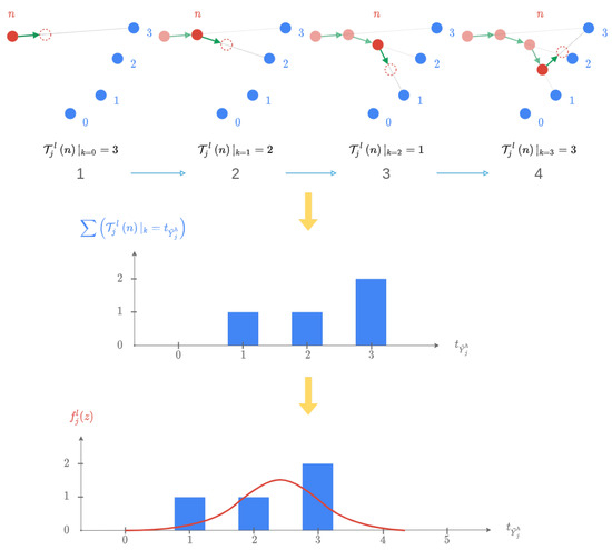
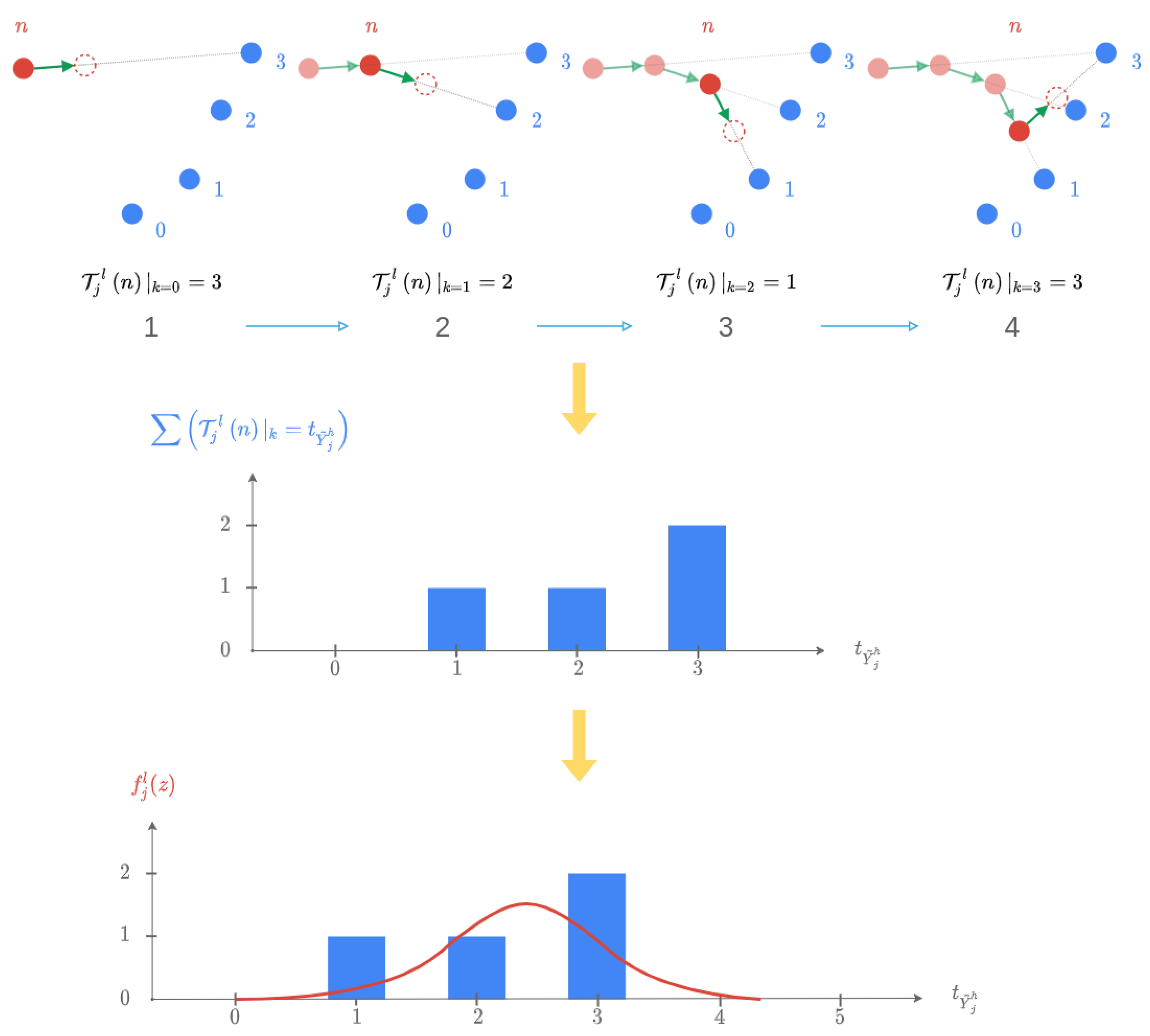
Figure 17.
Illustration of the uncertainty calculation method for iterations on the assignment of the nearest neighbor of the last point of on (restriction to 4 points).
Thus, a matrix representing the uncertainty by a probability density of the time index of the last aligned point for each descriptor has been obtained. It remains to weigh each of its columns by the elements of the vector . From the vector , it is possible to construct a matrix created by n concatenations of vectors on the lines. The matrix is then defined as . By defining the Hadamard product for two matrices, which allows the multiplication of the elements of two matrices term by term, by the symbol ⊙, the matrix is modified to create the matrix . The latter is thus defined by Equation (14).
This last step is illustrated by the schematic diagram in Figure 18 and the results for all the descriptors in Figure 19.
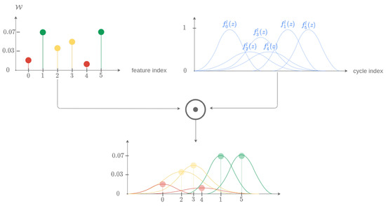
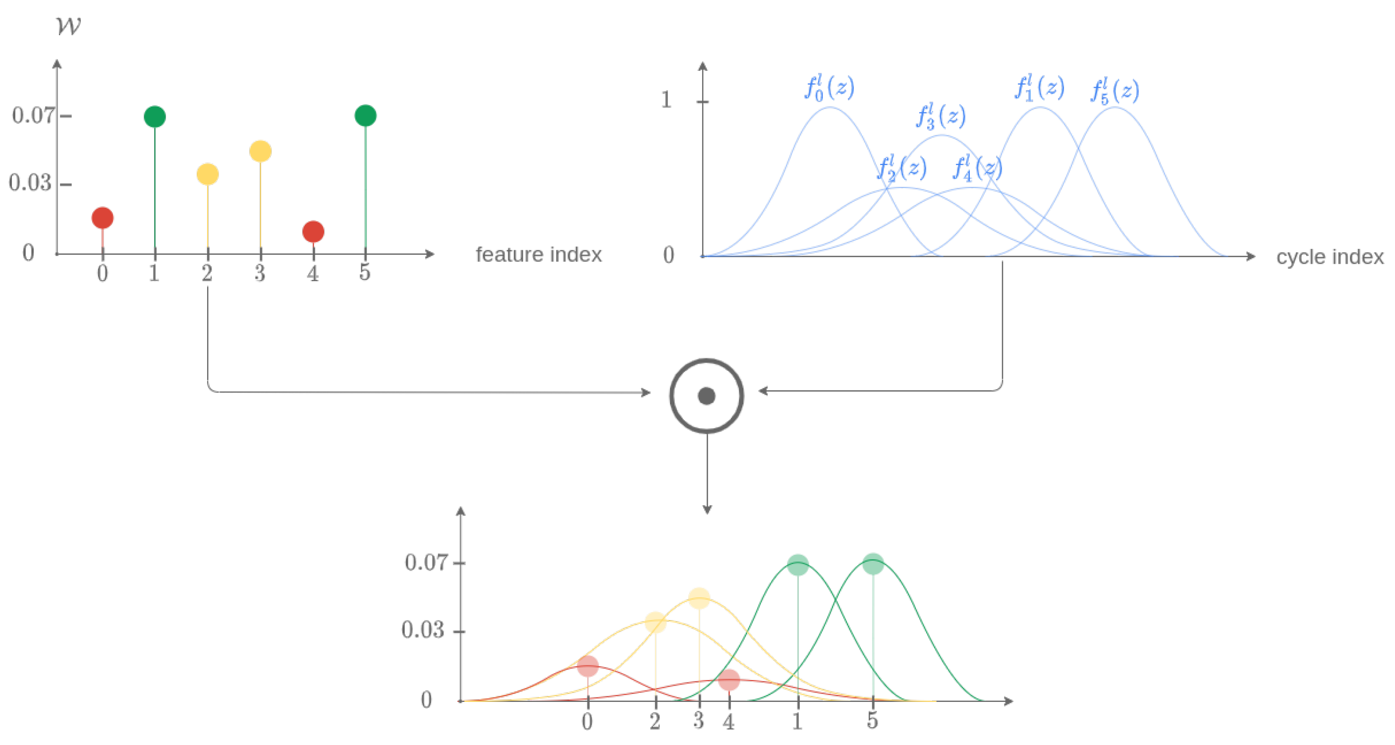
Figure 18.
Schematic diagram for the determination of intermediate probability densities before merging.
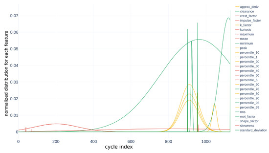
Figure 19.
Probability densities obtained for each descriptor during the alignment .
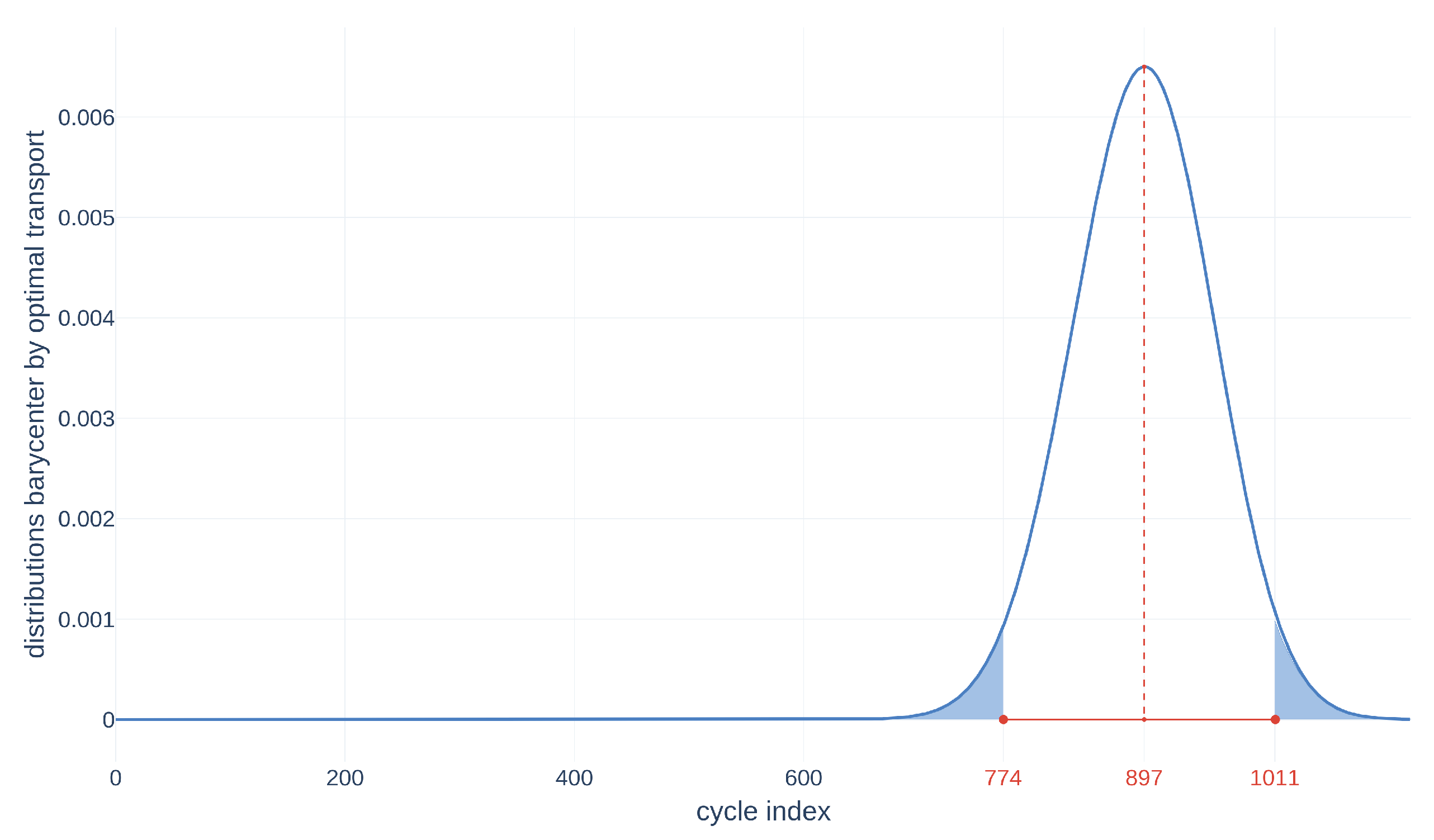
The last step is to merge all these distributions to obtain the RUL and the final distribution. We use the barycenter in the Wasserstein space [12,13] to obtain the RUL in Figure 20.
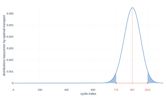
Figure 20.
Barycenter in Wasserstein space from the matrix for the alignment of the matrix on the tensor .
9. Conclusions
In conclusion, our research presents a novel and robust method for time series alignment-based prognostics, which is applicable to compressed or dilated time series, incomplete time series, or even series-independent segments, making it well suited for industrial applications. We have proposed a two-part method called Partial Time Scaling Invariant Temporal Alignment (PARTITA) that can align new data to the ones in our training data set without requiring the selection of a sliding window or any hyperparameters in advance.
The first part of our method involves an alignment algorithm that differs from the state-of-the-art methods in that it does not require the selection of an interval on which to align the time series and can align time series with different sampling frequencies. The second part involves the selection of the time index of every last point of each feature and assigning a density estimation for every one of them. Fusing every density by solving an optimal transport problem gives us the RUL of the studied system with an uncertainty measurement.
Our proposed method can potentially be applied to the diagnosis and prognosis of electromechanical actuators and any system’s behavior characterized by univariate time series in an industrial context. We believe that our approach offers a significant contribution to the field of prognostics and can be further extended to other applications as well.
Author Contributions
Conceptualization, A.E. and G.C.; methodology, A.E. and G.C.; software, A.E.; validation, A.E.; formal analysis, A.E.; investigation, A.E.; resources, B.M.; data curation, A.E.; writing—original draft preparation, A.E. and G.C.; writing—review and editing, A.E. and G.C.; visualization, A.E.; supervision, G.C. and B.M.; project administration, G.C. and B.M.; funding acquisition, B.M. All authors have read and agreed to the published version of the manuscript.
Funding
This research was funded by the French agency for research and technology (ANRT) through the CIFRE grant 2018/0649, by Safran Electronics & Defense (Safran Group) and by Laboratory Ampère CNRS—UMR5005, own funds.
Data Availability Statement
Restrictions apply to the availability of these data. Data were obtained from Safran Electronics & Defense and are not publicly available. Data sharing not applicable.
Conflicts of Interest
Authors Alexandre Eid and Badr Mansouri were employed by the company Safran Electronics & Defense (Safran Group). The remaining authors declare that the research was
conducted without any commercial or financial relationships that could be construed as a potential
conflict of interest.
Abbreviations
The following abbreviations are used in this manuscript:
| BGA | Ball Grid Array |
| CMAPSS | Commercial Modular Aero-Propulsion System Simulation |
| DTW | Dynamic Time Warping |
| LLA | Lower Left Actuator |
| LRA | Lower Right Actuator |
| PARTITA | Partial Time Scaling Invariant Temporal Alignment |
| PHM | Prognostics and Health Management |
| RMS | Root Mean Square |
| RUL | Remaining Useful Life |
| SBRLP | Similarity-Based Residual Life Prediction |
| SOH | State of Health |
| SPOT | Sliced Partial Optimal Transport |
| TBSP | Trajectory Similarity-Based Prediction |
| ULA | Upper Left Actuator |
| URA | Upper Right Actuator |
Appendix A. Detailed Algorithms
Appendix A.1. Quadratic Assignment for Two Time Series
| Algorithm A1 Quadratic assignment, from [11], Section 5 |
Input: , cloud points projected on direction n and m are source and target interval sizes Output: Assignment table representing the function
|
Appendix A.2. Nearest Neighbor Assignation for Two Time Series, Section 5
| Algorithm A2 Nearest neighbor assignation, from [11] |
Input: , two time series structure containing parameters of source and target segments to align Output: nnAssignArray is an assignment array of nearest neighbors of to
|
Appendix A.3. Advection from Source to Target Time Series, Section 5
| Algorithm A3 Advection from the source to the target |
Input: et are the source and target points nnAssignmentArray is the array of the closest neighbors from X to Y projSrcWIndex is the array of the projected source with the associated indices projTargetWIndex is the array of the projected target with the associated indices sigmoid contains two hyperparameters for the displacement, one for each dimension Output: is the cloud of source points transported on the target advectCost represents the movement cost, i.e., movement from source to target
|
Appendix A.4. Global Algorithm: Time Series Alignment, Section 5
| Algorithm A4 Time series alignment (first part) |
Input: and are source and target cloud points a list containing the two optimal projection directions (hyperparameters) weightArray an array containing weights (hyperparameters) Output: source cloud point moved towards the target cloud point
|
| Algorithm A5 Time series alignment (second part) |
|
References
- Atamuradov, V.; Medjaher, K.; Dersin, P.; Lamoureux, B.; Zerhouni, N. Prognostics and Health Management for Maintenance Practitioners—Review, Implementation and Tools Evaluation. Int. J. Progn. Health Manag. 2017, 8, 31. [Google Scholar] [CrossRef]
- Eid, A.; Clerc, G.; Mansouri, B.; Roux, S. A Novel Deep Clustering Method and Indicator for Time Series Soft Partitioning. Energies 2021, 14, 5530. [Google Scholar] [CrossRef]
- Sakoe, H.; Chiba, S. Dynamic programming algorithm optimization for spoken word recognition. IEEE Trans. Acoust. Speech Signal Process. 1978, 26, 43–49. [Google Scholar] [CrossRef]
- Mijatovic, N.; Peter, A.M. Curve Registration and Mean Estimation using Warplets. In Proceedings of the 1st International Conference on Advances in Signal Processing and Artificial Intelligence (ASPAI’ 2019), Barcelona, Spain, 20–21 March 2019. [Google Scholar]
- Wang, T.; Yu, J.; Siegel, D.; Lee, J. A Similarity-Based Prognostics Approach for Remaining Useful Life Estimation of Engineered Systems. In Proceedings of the 2008 International Conference on Prognostics and Health Management, Denver, CO, USA, 6–9 October 2008; pp. 1–6. [Google Scholar] [CrossRef]
- Saxena, A.; Goebel, K. Turbofan Engine Degradation Simulation Data Set; NASA: Washington, DC, USA, 2008. [Google Scholar]
- You, M.Y.; Meng, G. A Generalized Similarity Measure for Similarity-Based Residual Life Prediction. J. Process. Mech. Eng. 2011, 225, 151–160. [Google Scholar] [CrossRef]
- You, M.Y.; Meng, G. A Framework of Similarity-Based Residual Life Prediction Approaches Using Degradation Histories With Failure, Preventive Maintenance, and Suspension Events. IEEE Trans. Reliab. 2013, 62, 127–135. [Google Scholar] [CrossRef]
- El Jamal, D.; Al-Kharaz, M.; Ananou, B.; Graton, G.; Ouladsine, M.; Pinaton, J. Combining Approaches of Brownian Motion and Similarity Principle to Improve the Remaining Useful Life Prediction. In Proceedings of the 2021 IEEE International Conference on Prognostics and Health Management (ICPHM), Detroit, MI, USA, 7–9 June 2021; pp. 1–7. [Google Scholar] [CrossRef]
- You, M.Y.; Meng, G. Toward Effective Utilization of Similarity Based Residual Life Prediction Methods: Weight Allocation, Prediction Robustness, and Prediction Uncertainty. J. Process. Mech. Eng. 2013, 227, 74–84. [Google Scholar] [CrossRef]
- Bonneel, N.; Coeurjolly, D. SPOT: Sliced Partial Optimal Transport. ACM Trans. Graph. 2019, 38, 1–13. [Google Scholar] [CrossRef]
- Villani, C. Optimal Transport: Old and New; Grundlehren der Mathematischen Wissenschaften; Springer: Berlin/Heidelberg, Germany, 2009. [Google Scholar] [CrossRef]
- Agueh, M.; Carlier, G. Barycenters in the Wasserstein Space. SIAM J. Math. Anal. 2011, 43, 904–924. [Google Scholar] [CrossRef]


Disclaimer/Publisher’s Note: The statements, opinions and data contained in all publications are solely those of the individual author(s) and contributor(s) and not of MDPI and/or the editor(s). MDPI and/or the editor(s) disclaim responsibility for any injury to people or property resulting from any ideas, methods, instructions or products referred to in the content. |
© 2023 by the authors. Licensee MDPI, Basel, Switzerland. This article is an open access article distributed under the terms and conditions of the Creative Commons Attribution (CC BY) license (https://creativecommons.org/licenses/by/4.0/).