
Identification of Hydrodynamic Coefficients of the SUBOFF Submarine Using the Bayesian Ridge Regression Model
Abstract
:1. Introduction
2. Mathematical Model
2.1. Submarine Motion Equation
2.2. Bayesian Ridge Regression Model
3. Model and CFD Methods
3.1. Model
3.2. CFD Methods
3.3. Spatial Motion Simulation
3.3.1. Grid
3.3.2. Body Force Propeller Model
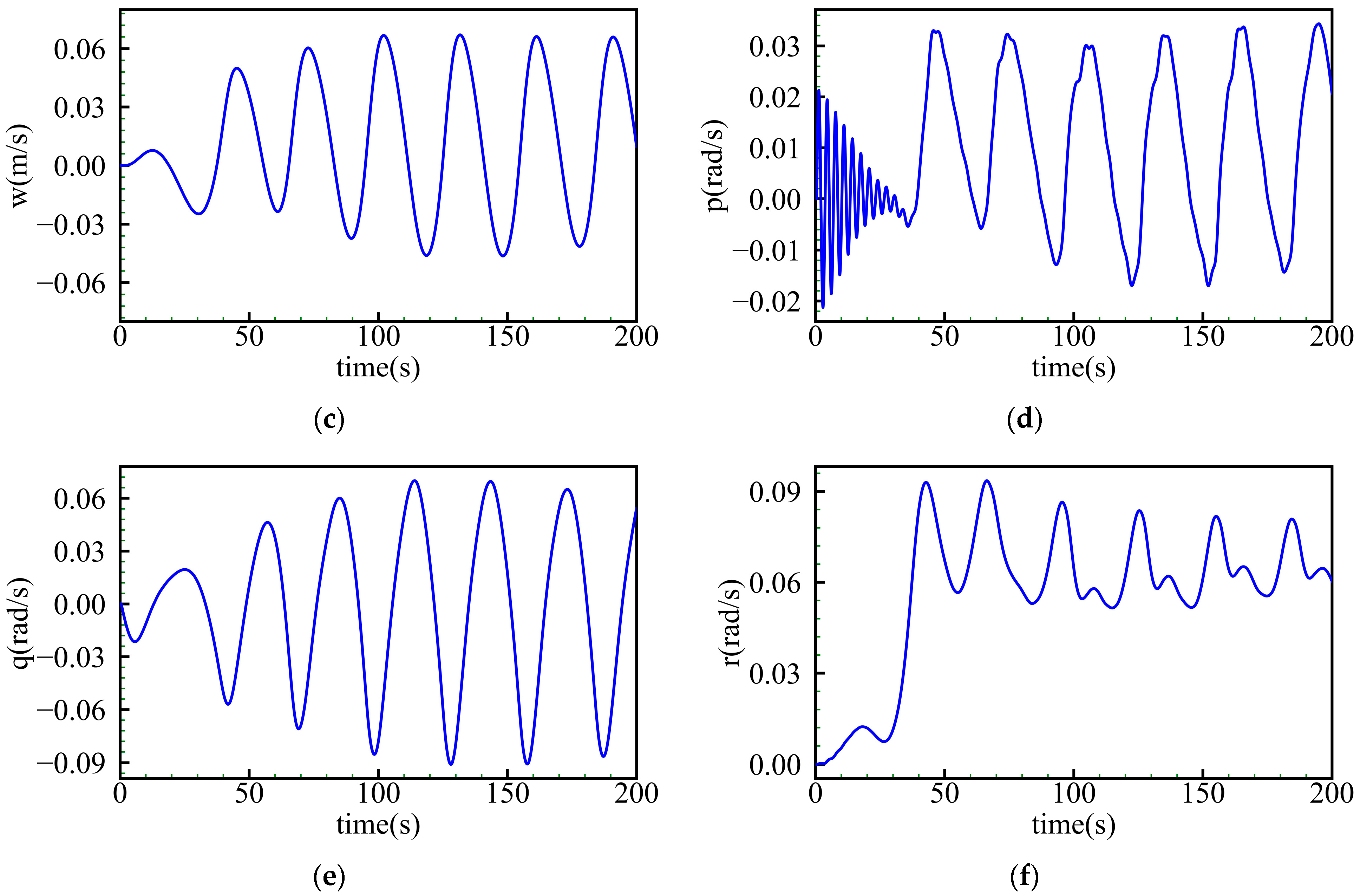
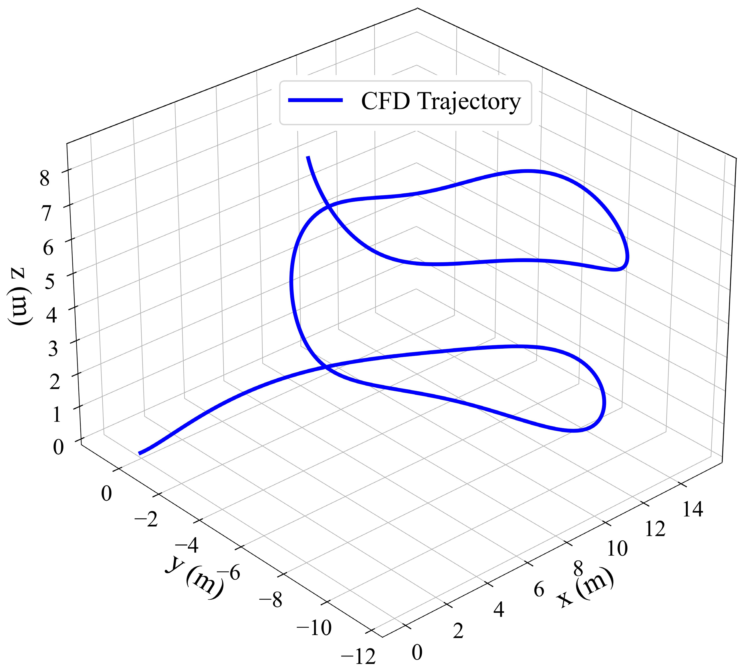
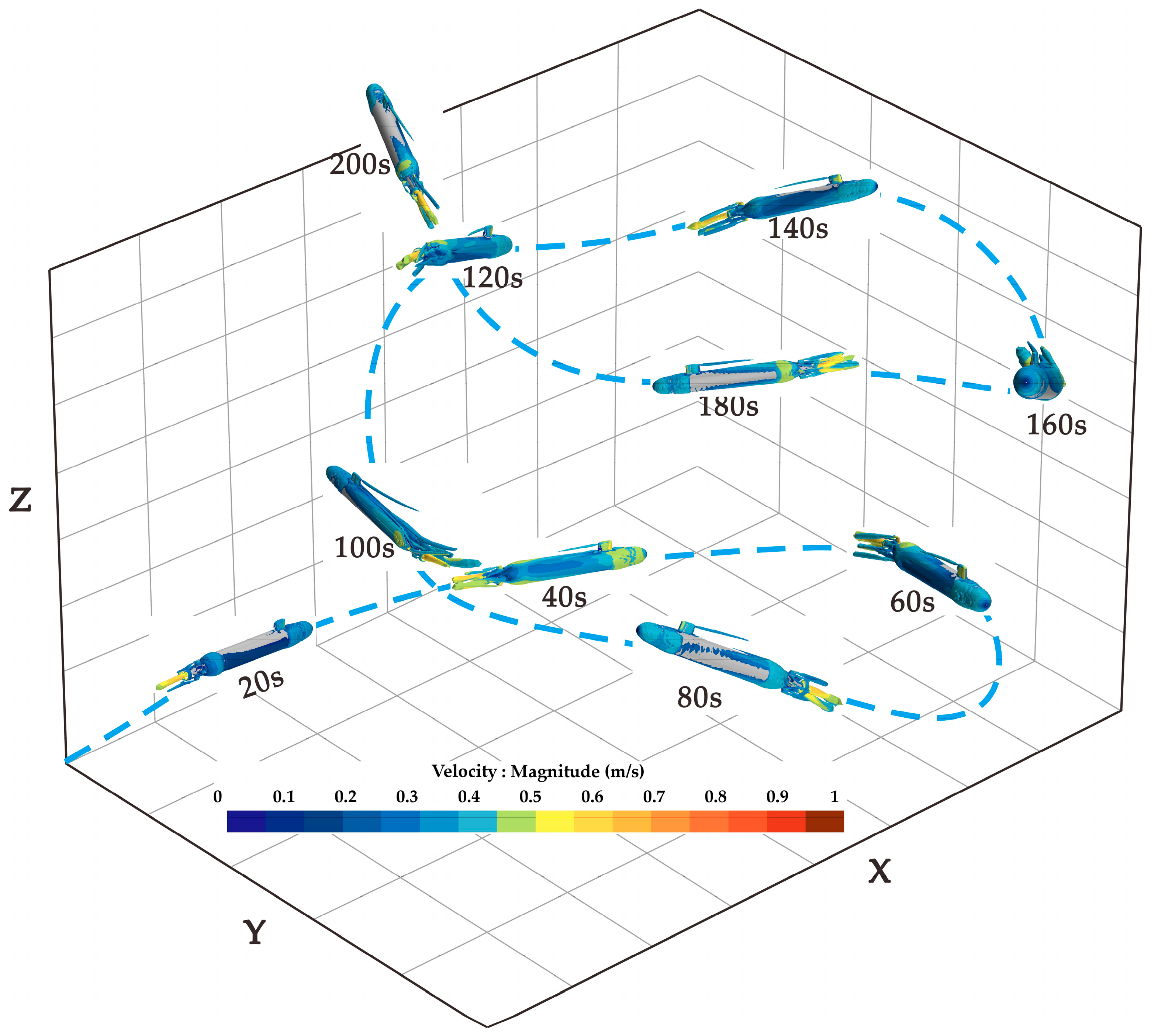
3.3.3. Spatial Motion Result
3.4. Simulated Restraint Model Test
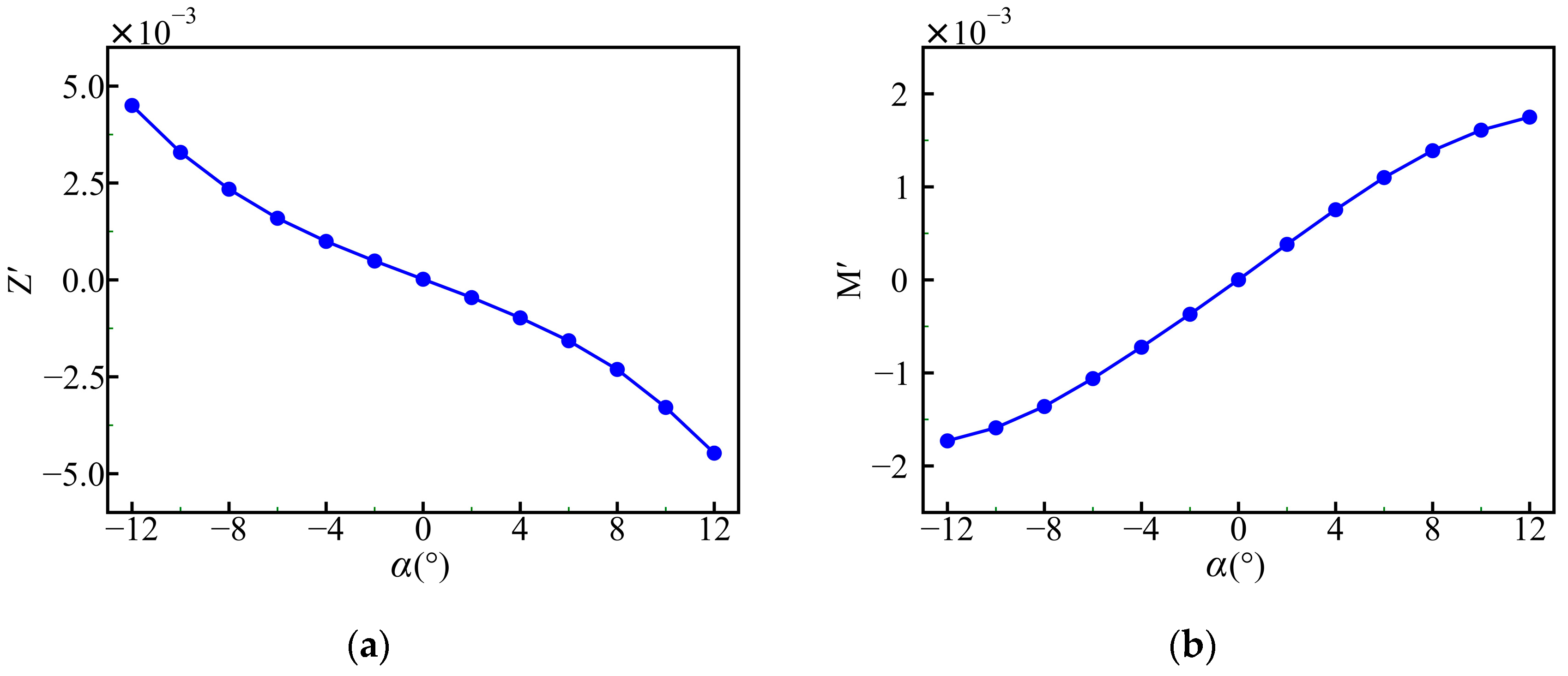
3.4.1. Oblique Towing Tests on the Vertical Plane
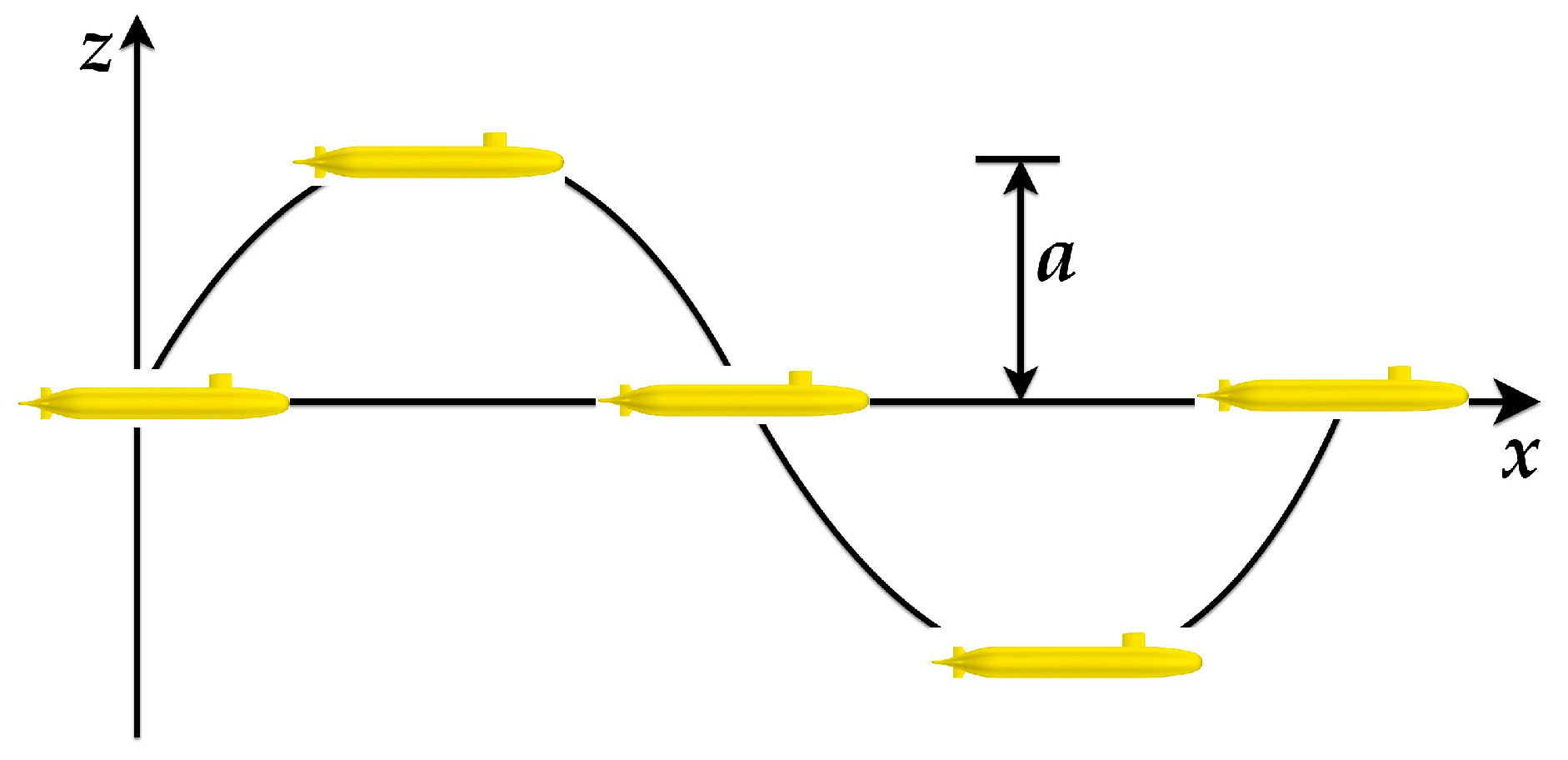
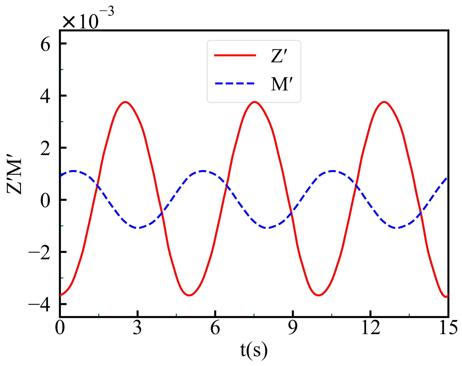
3.4.2. Pure Heaving
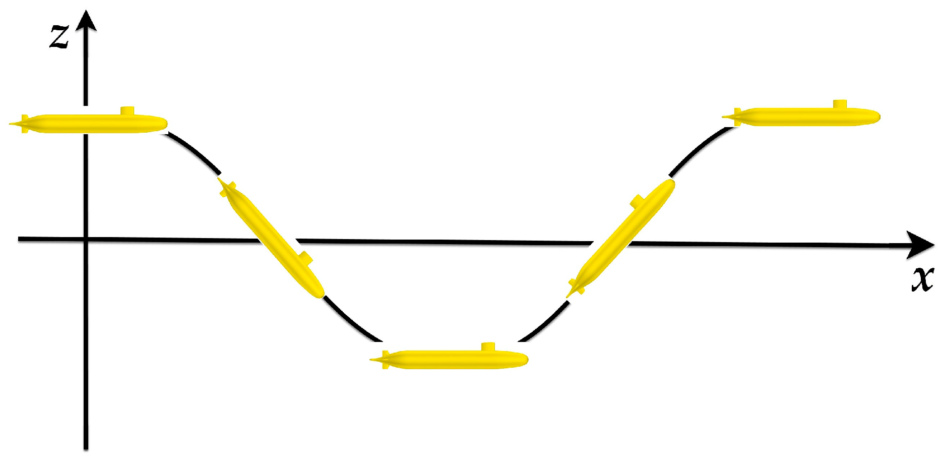
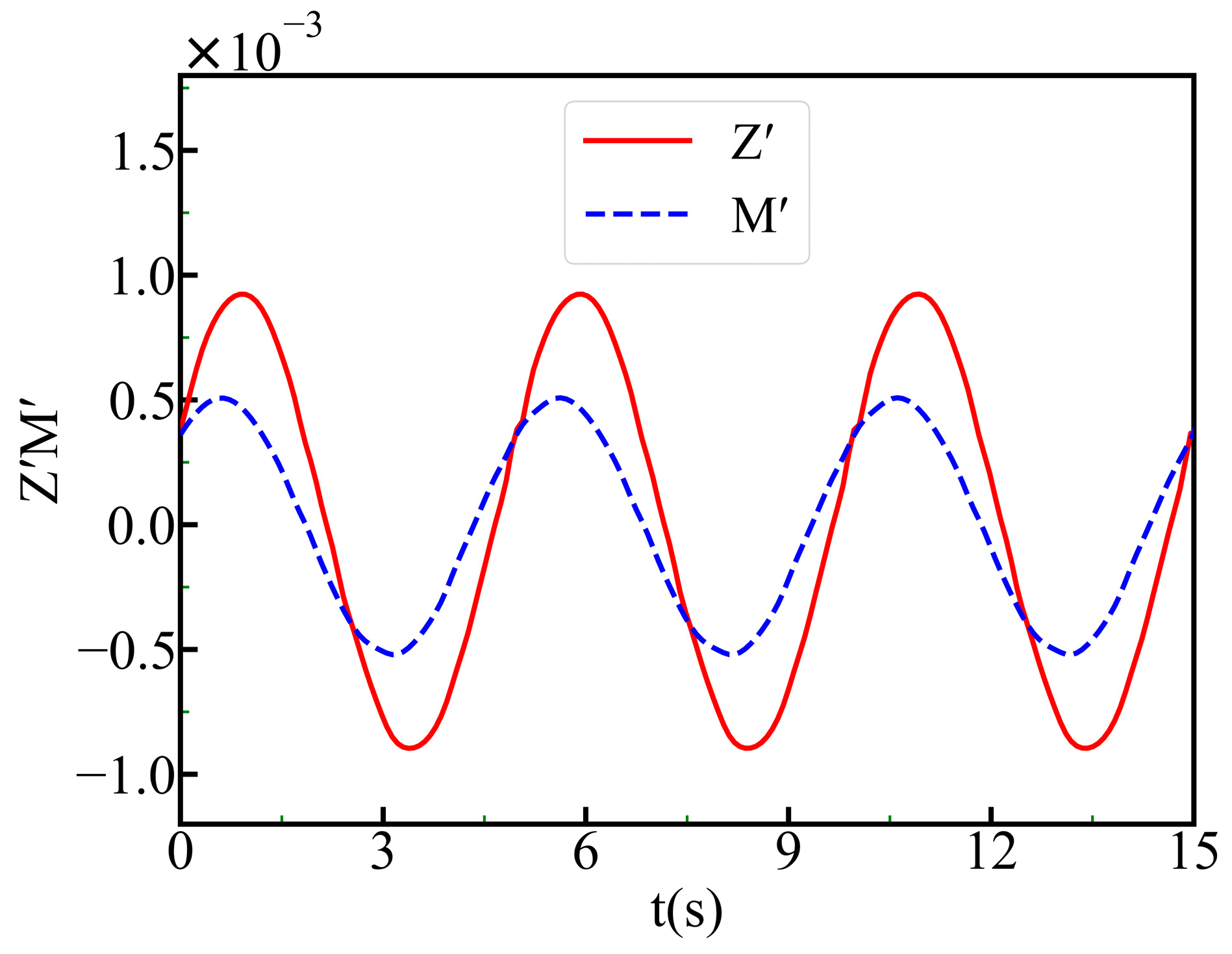
3.4.3. Pure Pitch
4. Results and Discussion
4.1. Results of Hydrodynamic Coefficient Identification
4.2. Spatial Motion Prediction and Analysis
5. Conclusions
Author Contributions
Funding
Institutional Review Board Statement
Informed Consent Statement
Data Availability Statement
Conflicts of Interest
References
- Gertier, M.; Hagen, G.E.; Hagen, G.R. Standard Equations of Motion for Submarine Simulation; NSRDC-2510; Naval Ship Research and Development Center: Bethesda, MD, USA, 1967. [Google Scholar]
- Dantas, J.L.D.; da Silva Caetano, W.; da Silva Vale, R.T.; de Oliveira, L.M.; Pinheiro, A.R.M.; de Barros, E.A. Experimental Research on Underwater Vehicle Manoeuvrability Using the AUV Pirajuba. In Proceedings of the International Congress of Mechanical Engineering (COBEM 2013), Ribeirão Preto, Brazil, 3–7 November 2013. [Google Scholar]
- Alex, G.; Morton, G. Planar Motion Mechanism and System. U.S. Patent US3052120A, 4 September 1962. [Google Scholar]
- Burcher, R.K. Co-operative tests for ITTC mariner class ship rotating arm experiments. In Proceedings of the 12th International Towing Tank Conference 1969, Rome, Italy, 22–30 September 1969. [Google Scholar]
- Kim, H.; Akimoto, H.; Islam, H. Estimation of the hydrodynamic derivatives by Rans simulation of planar motion mechanism test. Ocean Eng. 2015, 108, 129–139. [Google Scholar] [CrossRef]
- Ji, D.; Wang, R.; Zhai, Y.; Gu, H. Dynamic modeling of quadrotor AUV using a novel CFD simulation. Ocean. Eng. 2021, 237, 109651. [Google Scholar] [CrossRef]
- Wu, X.; Wang, Y.; Huang, C.; Hu, Z.; Yi, R. An effective CFD approach for marine-vehicle maneuvering simulation based on the hybrid reference frames method. Ocean Eng. 2015, 109, 83–92. [Google Scholar] [CrossRef]
- Gao, T.; Wang, Y.; Pang, Y.; Chen, Q.; Tang, Y. A time-efficient CFD approach for hydrodynamic coefficient determination and model simplification of submarine. Ocean. Eng. 2018, 154, 16–26. [Google Scholar] [CrossRef]
- Abkowitz, M.A. Measurement of hydrodynamic characteristic from ship maneuvering trials by system identification. SNAME Trans. 1980, 88, 283–318. [Google Scholar]
- Ebrahimi, S.; Bozorg, M.; Zare Ernani, M. Identification of an Autonomous Underwater Vehicle Dynamic Using Extended Kalman Filter with ARMA Noise Model. Int. J. Robot. 2015, 4, 22–28. [Google Scholar]
- Cardenas, P.; de Barros, E.A. Estimation of AUV Hydrodynamic Coefficients Using Analytical and System Identification Approaches. IEEE J. Ocean. Eng. 2019, 45, 1157–1176. [Google Scholar] [CrossRef]
- Sajedi, Y.; Bozorg, M. Robust estimation of hydrodynamic coefficients of an AUV using Kalman and H∞ filters. Ocean Eng. 2019, 182, 386–394. [Google Scholar] [CrossRef]
- Rasekh, M.; Mahdi, M. Combining CFD, ASE, and HEKF approaches to derive all of the hydrodynamic coefficients of an axisymmetric AUV. Proc. IME M J. Eng. Marit. Environ. 2022, 236, 474–492. [Google Scholar] [CrossRef]
- Sabet, M.T.; Daniali, H.M.; Fathi, A.; Alizadeh, E. Identification of an Autonomous Underwater Vehicle Hydrodynamic Model Using the Extended, Cubature, and Transformed Unscented Kalman Filter. IEEE J. Ocean. Eng. 2018, 43, 457–467. [Google Scholar] [CrossRef]
- Deng, F.; Levi, C.; Yin, H.; Duan, M. Identification of an Autonomous Underwater Vehicle hydrodynamic model using three Kalman filters. Ocean Eng. 2021, 229, 108962. [Google Scholar] [CrossRef]
- Liang, X.; Li, W.; Lin, J.; Su, L.; Li, H. Model Identification for Autonomous Underwater Vehicles Based on Maximum Likelihood Relaxation Algorithm. In Proceedings of the Second International Conference on Computer Modeling and Simulation, Sanya, China, 22–24 January 2010; IEEE: Darmstadt, Germany, 2010; pp. 128–132. [Google Scholar]
- Zhao, R.; Xie, H.; Qiao, B. A method for identifying hydrodynamic parameters of undersea vehicle based on test data. J. Unmanned Undersea Syst. 2018, 26, 335–341. [Google Scholar]
- Zhang, G.; Zhang, X.; Pang, H. Multi-innovation auto-constructed least squares identification for 4 DOF ship maneuvering modeling with full-scale trial data. ISA Trans. 2015, 25, 186–195. [Google Scholar] [CrossRef] [PubMed]
- Dinç, M.; Hajiyev, C. Identification of hydrodynamic coefficients of AUV in the presence of measurement biases. J. Eng. Mar. Environ. 2022, 236, 756–763. [Google Scholar] [CrossRef]
- Xue, Y.; Liu, Y.; Ji, C.; Xue, G. Hydrodynamic parameter identification for ship maneuvering mathematical models using a Bayesian approach. Ocean Eng. 2020, 195, 106612. [Google Scholar] [CrossRef]
- Xu, F.; Zou, Z.J.; Yin, J.C.; Cao, J. Identification modeling of underwater vehicles’ nonlinear dynamics based on support vector machines. Ocean Eng. 2013, 67, 68–76. [Google Scholar] [CrossRef]
- Wang, Z.; Zou, Z.; Soares, C.G. Identification of ship maneuvering motion based on nu-support vector machine. Ocean Eng. 2019, 183, 270–281. [Google Scholar] [CrossRef]
- Zhang, P.; Liu, C.; Hu, K.; Zhang, J. Research of Hydrodynamic Coefficients Identification for Submarine in Vertical Motions Based on APSO. In Proceedings of the 2020 IEEE International Conference on Mechatronics and Automation, Beijing, China, 13–16 October 2020. [Google Scholar]
- Tipping, M.E. Sparse Bayesian Learning and the Relevance Vector Machine. J. Mach. Learn. Res. 2001, 1, 211–244. [Google Scholar]
- MacKay, D.J.C. Bayesian Interpolation. Neural Comput. 1992, 4, 415–447. [Google Scholar] [CrossRef]
- Groves, N.; Huang, T.; Chang, M. Geometric Characteristics of DARPA (Defense Advanced Research Projects Agency) SUBOFF Models (DTRC Model Numbers 5470 and 5471); Technical Report; David Taylor Research Center: Bethesda, MD, USA, 1989.
- Celik, I.; Ghia, U.; Roache, P.J.; Freitas, C.; Coloman, H.; Raad, P. Procedure of Estimation and Reporting of Uncertainty Due to Discretization in CFD Applications. J. Fluids Eng. 2008, 130, 078001. [Google Scholar]
- Dantas, J.L.D.; de Barros, E.A. Numerical analysis of control surface effects on AUV manoeuvrability. Appl. Ocean Res. 2013, 42, 168–181. [Google Scholar] [CrossRef]
- Menter, F.R. Two-Equation Eddy-Viscosity Transport Turbulence Model for Engineering Applications. AIAA J. 1994, 32, 1598–1605. [Google Scholar] [CrossRef]
- Liu, H.-L.; Huang, T. Summary of DARPA Suboff Experimental Program Data; Naval Surface Warfare Center, Carderock Division (NEWCCD): Bethesda, MD, USA, 1998; Volume 28.
- Zhang, N.; Shen, H.; Yao, H. Uncertainty analysis in CFD for resistance and flow field. J. Ship Mech. 2008, 12, 211. [Google Scholar]
- Han, K.; Cheng, X.; Liu, Z.; Huang, C.; Chang, H.; Yao, J.; Tan, K. Six-DOF CFD Simulations of Underwater Vehicle Operating Underwater Turning Maneuvers. J. Mar. Sci. Eng. 2021, 9, 1451. [Google Scholar] [CrossRef]
- Oda, J.; Yamazaki, K. Technique to Obtain Optimum Strength Shape by the Finite Element Method: On Body Force Problem. Trans. Jpn. Soc. Mech. Eng. 1978, 44, 1141–1150. [Google Scholar] [CrossRef]
- Yeo, D.J.; Rhee, K.P. Sensitivity analysis of submersibles’ maneuverability and its application to the design of actuator inputs. Ocean Eng. 2006, 33, 2270–2286. [Google Scholar] [CrossRef]


| Parameter | Symbol | Unit | Value |
|---|---|---|---|
| Total length | L | m | 2.178 |
| Diameter | D | m | 0.254 |
| Sail length | LS | m | 0.184 |
| Sail height | LD | m | 0.112 |
| Mass of model | ms | kg | 88.02 |
| Center of mass | (xg, yg, zg) | m | (1.005, 0.0, −0.003) |
| Center of buoyancy | (xb, yb, zb) | m | (1.005, 0.0, 0.001) |
| Moment of inertia | (Ixx, Iyy, Izz) | kg·m2 | (0.88, 25.43, 25.43) |
| Method | Grid Level | Cells (Millions) | Drag Force (N) | Relative Error (%) |
|---|---|---|---|---|
| Experiment | - | - | 283.8 | - |
| CFD | Coarse | 2.96 | 299.87 | 5.66% |
| Medium | 7.25 | 291.76 | 2.81% | |
| Fine | 16.78 | 290.57 | 2.39% |
| Parameter | Symbol | Value |
|---|---|---|
| Blades | - | 5 |
| Diameter | DP | 0.15 |
| Hub-to-diameter ratio | d/DP | 0.2 |
| Disk aspect ratio | Ae/A0 | 0.725 |
| Force Direction | R2 | Force Direction | R2 |
|---|---|---|---|
| X | 0.985 | K | 0.989 |
| Y | 0.997 | M | 0.973 |
| Z | 0.987 | N | 0.964 |
| Coefficients | Bayesian × 10−4 | Coefficients | Bayesian × 10−4 | Coefficients | Bayesian × 10−4 |
|---|---|---|---|---|---|
| X | −8.31 | Z | −8.39 | M | −17.2 |
| Xuu | −11.0 | Zvr | −453.8 | Mq | −34.35 |
| Xvv | 171.6 | Zq | −71.47 | Mw | 98.99 |
| Y | −141.68 | Zw | −144.05 | Mvr | −5.2 |
| Y | −5.11 | K | −0.52 | Mδs | −36.66 |
| Y | 4.47 | K | −0.03 | N | 2.92 |
| Yr | 57.05 | Kp | −4.8 | N | −7.31 |
| Yp | −29.7 | Kr | 2.6 | N | −0.086 |
| Yv|r| | 4.5 | Kwr | 11.3 | Nr | −46.31 |
| Yv | 280.76 | Kv | −6.46 | Nv | −145.05 |
| Yv|v| | −1160.1 | Kδr | −0.1 | N|v|r | −20.8 |
| Yδr | 71.43 | Z|w| | −20.0 | Nδr | −26.83 |
| Yvw | −3025.7 | Zδs | −49.21 | ||
| Z | −115.55 | M | −2.85 |
| Coefficients | CFD × 10−4 | Bayesian × 10−4 | Errors Compared to CFD Method % |
|---|---|---|---|
| Zw | −131.85 | −144.05 | 9.25 |
| Mw | 95.34 | 98.99 | 3.82 |
| Zq | −71.32 | −79.43 | 11.37 |
| Mq | −35.59 | −34.35 | −3.49 |
| Z | −110.19 | −115.55 | 4.87 |
| M | −5.02 | −2.85 | −43.26 |
| Z | −7.68 | −8.39 | 9.30 |
| M | −7.88 | −7.39 | −6.21 |
| Zδs | - | −49.21 | - |
| Mδs | - | −36.66 | - |
| Yv | 261.14 | 280.76 | 7.51 |
| Nv | −142.96 | −145.05 | 1.46 |
| Kv | - | −6.46 | - |
| Yr | 57.35 | 57.05 | −0.53 |
| Nr | −50.20 | −46.31 | −7.75 |
| Y | −139.94 | −141.68 | 1.24 |
| N | 2.57 | 2.92 | 13.76 |
| Y | 4.32 | 4.47 | 3.47 |
| N | −7.96 | −7.31 | −8.11 |
| Yδr | - | 71.43 | - |
| Nδr | - | −26.83 | - |
| Kδr | - | −0.10 | - |
Disclaimer/Publisher’s Note: The statements, opinions and data contained in all publications are solely those of the individual author(s) and contributor(s) and not of MDPI and/or the editor(s). MDPI and/or the editor(s) disclaim responsibility for any injury to people or property resulting from any ideas, methods, instructions or products referred to in the content. |
© 2023 by the authors. Licensee MDPI, Basel, Switzerland. This article is an open access article distributed under the terms and conditions of the Creative Commons Attribution (CC BY) license (https://creativecommons.org/licenses/by/4.0/).
Share and Cite
Xiang, G.; Ou, Y.; Chen, J.; Wang, W.; Wu, H. Identification of Hydrodynamic Coefficients of the SUBOFF Submarine Using the Bayesian Ridge Regression Model. Appl. Sci. 2023, 13, 12342. https://doi.org/10.3390/app132212342
Xiang G, Ou Y, Chen J, Wang W, Wu H. Identification of Hydrodynamic Coefficients of the SUBOFF Submarine Using the Bayesian Ridge Regression Model. Applied Sciences. 2023; 13(22):12342. https://doi.org/10.3390/app132212342
Chicago/Turabian StyleXiang, Guo, Yongpeng Ou, Junjie Chen, Wei Wang, and Hao Wu. 2023. "Identification of Hydrodynamic Coefficients of the SUBOFF Submarine Using the Bayesian Ridge Regression Model" Applied Sciences 13, no. 22: 12342. https://doi.org/10.3390/app132212342