Multi-View Masked Autoencoder for General Image Representation

Abstract

Self-supervised learning is a method that learns general representation from unlabeled data. Masked image modeling (MIM), one of the generative self-supervised learning methods, has drawn attention for showing state-of-the-art performance on various downstream tasks, though it has shown poor linear separability resulting from the token-level approach. In this paper, we propose a contrastive learning-based multi-view masked autoencoder for MIM, thus exploiting an image-level approach by learning common features from two different augmented views. We strengthen the MIM by learning long-range global patterns from contrastive loss. Our framework adopts a simple encoder–decoder architecture, thus learning rich and general representations by following a simple process: (1) Two different views are generated from an input image with random masking and by contrastive loss, we can learn the semantic distance of the representations generated by an encoder. By applying a high mask ratio, of 80%, it works as strong augmentation and alleviates the representation collapse problem. (2) With reconstruction loss, the decoder learns to reconstruct an original image from the masked image. We assessed our framework through several experiments on benchmark datasets of image classification, object detection, and semantic segmentation. We achieved 84.3% in fine-tuning accuracy on ImageNet-1K classification and 76.7% in linear probing, thus exceeding previous studies and showing promising results on other downstream tasks. The experimental results demonstrate that our work can learn rich and general image representation by applying contrastive loss to masked image modeling.

1. Introduction

Deep learning, which has been revolutionized over the past decade, has recently faced data-hungry problems due to the rapid growth of hardware and resources [1,2,3]. Self-supervised learning, which learns meaningful data representations from unlabeled data [4], has emerged as an alternative to supervised learning resulting from the inefficiency of labeling in terms of time and labor [5,6,7].

Masked autoencoding [8] is a method that learns representations by removing part of the input and predicting the masked part. Autoencoder [9,10] architecture is used for masked autoencoding, thus compressing high-dimensional data into a latent representation with an encoder and reconstructing the original data with a decoder, as shown in Figure 1. It has been successful in NLP as a method of self-supervised pre-training. The approach of learning representation by reconstructing images from corrupted images is not new; the idea was already proposed before 2017 [11,12]. The idea was buried after the emergence of contrastive learning, since it has shown promising results on downstream tasks [13,14,15]. Upon witnessing the success of masked autoencoding in NLP fields [16,17,18], many works tried to apply masked autoencoding to vision, but they lagged behind due to the following reasons: (1) In vision, convolutional network architecture has been dominant [19], where indicators like mask token [17] or positional embedding [20] are inapplicable. (2) With only a few neighboring pixels, missing parts of an image can be successfully predicted without a deep understanding of an image [21]. However, when predicting a missing part/token, complex language understanding should be investigated. In other words, the masked autoencoding in the vision field might not demand fully understanding the image, which results in capturing less useful features. Due to these differences between the two modalities, masked autoencoding has been limitedly applied in the vision field until the advent of the vision transformer (ViT) [22].

Motivated by the success of masked language modeling (MLM) in language understanding, masked image modeling (MIM), following the idea of MLM, learns rich and holistic representations by reconstructing masked original information (e.g., pixel and representation) from unmasked information. MIM has gained much importance recently by showing state-of-the-art performance [2,23,24] not only in ImageNet classification, but also in other downstream tasks like object detection and semantic segmentation.

Before MIM, contrastive learning (CL), which learns meaningful representation by using similarities and differences between image representations, was a dominant method in self-supervised learning [4]. By learning embedding space in a way that contrasts each other so that positive samples are located close and negative samples are far away, CL learns to discriminate instances using features of the entire image [25]. Contrary to CL, MIM does not learn instance discriminativeness, since it only considers relationships between patches or pixels through the image reconstruction task [26]. Therefore, although MIM methods exceed the performance of CL methods in fine-tuning, they are shown to be less effective in linear separability.

In this work, we propose a simple yet effective framework, thus adopting multi-view autoencoder architecture and utilizing contrastive learning for MIM to overcome the gap between CL and MIM. Different from conventional autoencoder architectures are shown in Figure 1; we add an additional branch to learn common information from two different augmented views by contrasting different images originating from the same image. We call this architecture a multi-view autoencoder. CL learns instance discriminative representations to result in better performance in linear probing, while MIM shows better performance in fine-tuning settings. We note that the proposed contrastive learning-based MIM method can strengthen MIM by learning global patterns of an image with contrastive loss, which is in contrast to the existing pixel-level approaches that only learn local representations of images.

In more detail, we adopt an asymmetric encoder–decoder architecture using ViT [22] blocks. The ViT makes the model focus on important features of an instance. We visualized maps of the attention of our pre-trained ViT encoder as shown in Figure 2, thus taking the average of the ViT heads following the work of [27]. CL is used to capture global information and learn discriminative representation by contrasting negative samples while pulling positive samples. By generating two augmented views via masking, with the encoder, we compress them into latent representations, which are used for contrastive loss. While learning holistic information from contrastive loss, reconstruction loss helps the decoder to learn local representation by predicting patches from the masked image.

We conducted experiments to prove the effectiveness of our work. The proposed method is a pre-training method, and we only used a pre-trained ViT encoder during fine-tuning. Our ViT encoder pre-trained with the proposed method exceeds previous work, thereby showing 84.3% ImageNet-1K classification top-1 accuracy. Though showing lower performance, but comparable compared to other CL-based methods in linear probing, our work shows an impressive performance gain compared to MIM methods by achieving a 76.7% accuracy. We also evaluated the transfer learning on object detection and segmentation. We recorded a 51.3% AP${}^{box}$ and a 45.6% AP${}^{mask}$ on COCO, as well as a 50.2% mIOU on ADE20K, which yielded the best and second best performance outcomes, respectively, compared to previous studies. Through ablation studies, we demonstrate that utilizing CL for MIM helps the model learn better representation.

Our contributions are summarized as follows:

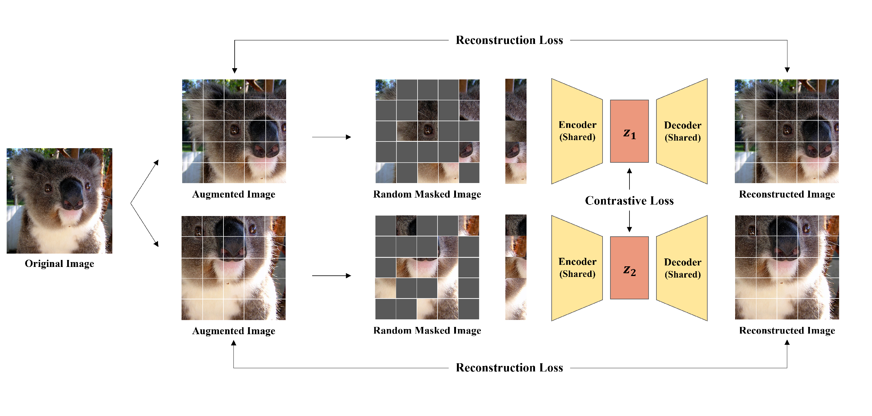
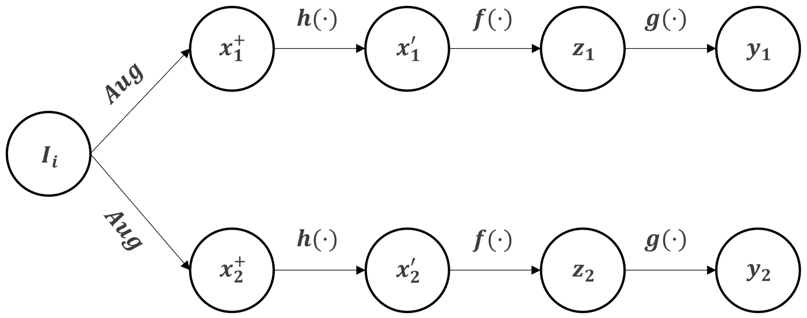
• We propose a simple framework exploiting contrastive learning for MIM to learn rich and holistic representations. The model learns discriminative representation by contrasting two augmented views while reconstructing original signals from the corrupted ones.
• A high masking ratio works as strong augmentation. Without additional augmentation like color distortion, blur, etc., our model shows better performance than previous CL-based methods by only using masking and random cropping.
• Experimental results prove that our work is effective, thus outperforming previous MIM methods in ImageNet-1K classification, linear probing, and other downstream tasks like object detection and instance segmentation.

The rest of this paper is structured as follows. Section 2 introduces related works. In Section 3, we give an overview and details of our framework. Then, we show the experimental results and analysis in Section 4. Finally, Section 5 concludes the paper.

2. Related Work

2.1. Contrastive Learning

Contrastive learning [13,14,15,28,29,30] is a method of learning instance discriminative features by contrasting samples against each other to learn common features between data, which is categorized as discriminative self-supervised learning. CL has been a dominant self-supervised learning method [26], since it has demonstrated overwhelming performance over supervised learning. CL relies on negative samples and strong data augmentations to avoid the representation collapse problem, thus outputting constantly when given different inputs. Previous studies have investigated the use of memory banks [15] and large batch size [13] for better informative negative samples. Recent works have shown that, without discriminating between images, we can learn features by only using positive samples. BYOL [29] and SimSiam [31] use only positive samples in a different way; BYOL uses a momentum encoder, while SimSiam uses a stop gradient. Recent studies [14,32] that exploit the use of ViT architecture stand out compared to convolutional neural networks. The makers of DINO [14] discovered that ViT features contain explicit information about the semantic segmentation of an image and outperform previous self-supervised methods.

2.2. Masked Language Modeling

Masked language modeling (MLM) [16,17,18] is one of the most-used approaches for pre-training and shows promising results on various downstream tasks in NLP. GPT [16,33] and BERT [17] are the foundation models in MLM, but they have differences: BERT [17] uses entire words all at once using special mask tokens, while GPT [16] predicts the next word with previous words in an auto-regressive manner. They both remove a portion of text tokens and predict the removed part, which makes the model learn the context understanding of language by masking some parts [8].

2.3. Masked Image Modeling

In early works of masked image modeling (MIM), a denoising autoencoder [11,12] was introduced to restore blurred, masked pixels to original clean pixels. MIM studies [2,34] inspired by the successful context understanding of the masked parts in MLM tasks have been introduced. In [34], sequences of pixels were used to predict unknown pixels. BEiT [2] and MAE [23] are foundation models of MIM showing promising results on several downstream tasks. BEiT utilizes BERT-style pre-training by reconstructing visual tokens using a pre-trained dicrete VAE [35] as a tokenizer, while MAE predicts pixels directly using a ViT [22]. Also, ref. [36] improved segmentation performance through pre-training to predict pixels from masked pixels. Recent works have explored pixel or feature regression, though only in a relatively small model. The work of [37] proposes a model employing an enhancer network to either recover original image pixels or predict whether each visual token is replaced by a generator sample or not.

3. Method

3.1. Framework

The overall framework is shown in Figure 3, which adopts an autoencoder architecture. We propose contrastive learning to learn representation using multi-view of an image, thus using contrastive learning on latent representations of shared encoder. We generate multi-view of an image by simple augmentation with random masking. With encoder, we compress high-dimensional image data into low-dimensional latent representations and reconstruct the original images given latent representations with decoder. In detail, firstly, with random masking, two different masked images are generated from an input image. Encoder, consisting of ViT layers, takes two masked images as input, thus compressing them into latent representations, which are used for contrastive learning. Afterwards, decoder reconstructs the original image from latent representations with mask tokens. The training process is specified below.

3.1.1. Input and Target Views

We randomly sample N images in every iteration when pre-training. To create target views, denoted as $x_i^{+}\in {\mathbb{R}}^{224\times 224}$, we apply simple data augmentation, random resized cropping, and horizontal flipping. Also, we exploit applying augmentation two times, thus creating two different target views for effective use of contrastive learning as shown in Figure 4. Two different target views make the model see an input image from different points of view. The process of how target views are generated is shown in Figure 5.

3.1.2. Patchify and Masking Strategy

Since we adopt ViT for the encoder, we patchify the target views into a non-overlapping 14 × 14 patch sequence. To retain spatial information about where each patch is located, we add positional embedding to them. For positional encoding, we used sine–cosine positional encoding. In addition, for augmented view, we apply random masking to the patches. Masking is simple; we generate numbers following a uniform distribution. Afterwards, we ’mask’ a specific ratio of the total number of patches in the embedded patch sequence using the generated random numbers, i.e., random masking. The randomly masked patch sequences are denoted as $x_i^{\prime }\in {\mathbb{R}}^{m\times }$ and can be formulated as $x_i^{\prime }=h\left(x_i^{+}\right),i\in \{1,2\}$, where h denotes the patchifying and masking operation.

Conventionally, masked language models mask relatively low portion of tokens, because more masking would result in insufficient context to learn good representation [38]. However, because image pixels are continuous contrary to discrete language tokens, higher masking ratio should be applied to eliminate redundancy in image. We choose certain masking ratio through experiments; see Section 4.2.1.

3.1.3. Encoder

Our encoder $f(·)$ adopts ViT architecture, specifically ViT base with patch size 16. Each masked image $x_1^{\prime }$ and $x_2^{\prime }$ can be decomposed into visible patches and masked patches. They can be formulated as follows:

$$x_i^{\prime }\stackrel{}{\to }{x}_i^v,x_i^m$$

(1)

$$z_i=f(x_i^v+x_{pos})=ViT(x_i^v+x_{pos})$$

(2)

where $x_i^v$, $x_i^m$, and $x_{pos}$ are visible patches, masked patches, and positional embeddings, respectively. A whole process of encoder is shown in Figure 6. Specifically, for encoder input, as represented in Equation (2), only visible patches and positional encoding are passed through to generate latent representations denoted as $z_1$ and $z_2$, thus excluding masked patches in line with MAE, which allows for computing efficiency. Since ViT operates on image patches and uses self-attention mechanisms, which results in more computational complexity compared to CNNs, we should consider computational efficiency. We excluded masked patches, which means only 20% of image patches were computed with 80% of masking ratio.

The encoder learns to compress high-dimensional vectors retaining important information representing the given input data. We use latent representation, the output of the encoder, for contrastive learning by pulling the positive pairs close and pushing the negative pairs away. Using two different target views, mentioned in Section 3.1.1, strengthens the encoder to better learn instance discriminativeness by using different points of view. Also, since we aim to learn global patterns of an image, encoder learns to capture patterns that represents an image with visible patches by operating only on unmasked patches in encoder.

3.1.4. Decoder

To perform the reconstruction task, the decoder, $g(·)$, reconstructs images from given inputs $z_1$ and $z_2$ as shown in Figure 7. Our decoder also adopts ViT, but it is lightweight compared to the encoder. Given $z_1$ and $z_2$ as inputs, mask tokens are added, since our decoder computes over full patches. Also, we add positional embeddings to them. By doing so, mask tokens do know where they should be located. Following the setting of MAE, we also adopt an asymmetric encoder–decoder design, thus having a shallow depth of decoder. As our goal is to learn image representation, not reconstruct corrupted images, the decoder was only used in pre-training.

3.2. Training Objectives

For the training objective, we use two objectives: reconstruction loss and contrastive loss. Both loss functions are specified below.

3.2.1. Reconstruction Loss

We use reconstruction loss, mean squared error (MSE), as one of our training objectives, which is generally used in MIM. The model performs a pre-text task to reconstruct the original images from corrupted (here we say masked) ones. Given $y_1$ and $y_2$, prediction from the model, reconstruction loss computes over patchified target image $x_i^{+}$, which is formulated as follows:

$$\begin{array}{c}{\mathcal{L}}_r=\frac{1}{2N}\sum _{j=1}^N\sum _{i=1}^2{(y_i-x_i^{+})}^2\end{array}$$

(3)

where N is batch size. We divide MSE over twice the batch size, because two different views are generated from one image. This loss helps the model to learn local representations of images, since it uses neighboring patches to predict the masked ones.

3.2.2. Contrastive Loss

For contrastive loss, we use NT-Xent (the normalized temperature-scaled cross-entropy loss) proposed in [13]. This loss operates cosine similarity between given pairs, thus computing mutual information between them. In a mini-batch of N samples, images augmented from the same image are regarded as a positive pair and the rest of the samples, $2(N-1)$, are treated as negative samples. Contrastive loss is defined as follows:

$$\ell (i,j)=-log\frac{exp(sim(z_i,z_j)/\tau )}{{\sum }_{k=1}^{2N}{\mathbb{l}}_{[k\ne i]}exp(sim(z_i,z_k)/\tau )}$$

(4)

$$sim(i,j)=z_i^{\top }{z}_j/(\parallel z_i\parallel \parallel z_j\parallel )$$

(5)

$${\mathcal{L}}_c=\frac{1}{2N}\sum _{k=1}^N\{\ell (2k-1,2k)+\ell (2k,2k-1)\}$$

(6)

where ${\mathbb{l}}_{[k\ne i]}\in \{0,1\}$ is an indicator representing 1 if $k\ne i$ and $\tau$ denotes temperature constant. $\tau$ is set to 0.07, thus following the default setting of [13]. The denominator of $\ell (i,j)$ computes similarity over a positive pair, and the final contrastive loss function, ${\mathcal{L}}_c$, is computed across all positive pairs. By doing so, different views from the same image, which we call positive samples, are pulled together while pushing away negative samples in embedding space.

The total loss $\mathcal{L}$ is a weighted sum of reconstruction loss ${\mathcal{L}}_r$ and contrastive loss ${\mathcal{L}}_c$, which is formulated as follows:

$$\begin{array}{c}\mathcal{L}={\mathcal{L}}_r+\lambda {\mathcal{L}}_c\end{array}$$

(7)

where $\lambda$ is a hyperparameter deciding loss weight. The combination of two losses, reconstruction loss, and contrastive loss, contributes to learning image representation in a different way: reconstruction loss computes over the reconstructed images (i.e., model prediction), and the aimed target images learn local patterns of an image by reconstructing original information from corrupted ones. Contrastive loss computes over latent representations generated from the encoder and learns to capture instance discriminative representations of an image. By jointly using them, the model learns rich representations considering both global and local patterns of an image.

4. Experiments

4.1. Implementation Details

We pre-trained our model at 224 × 224 resolution on an ImageNet-1K [39] training set without labels. ImageNet-1K is a benchmark dataset for image classification consisting of about 1.2M training images and 50K validation set with 1000 classes. It is commonly used for pre-training due to its high quality and diversity of instances. After pre-training, we conducted several experiments to evaluate the proposed method. We fine-tuned our pre-trained model on the ImageNet dataset and conducted experiments on linear probing for analyzing the linear separability. To assess the transferability of the model, we used the COCO [40] and ADE20K [41] benchmark datasets for object detection, instance segmentation, and semantic segmentation. The implementation details are specified below.

4.1.1. Pre-Training

Most of the settings followed the MAE [23]. In detail, we applied random resized cropping and random horizontal flipping for augmentation. They were resized to be 224 × 224 so they could be divided into 16 × 16 patches. For the encoder, we used ViT-Base [22] with a 12-layer transformer with a 768 hidden size. We adopted the AdamW optimizer with ${\beta }_1$ = 0.9 and ${\beta }_2$ = 0.95 for optimization. The learning rate was set to 1.5 × 10${}^{-4}$, with a warmup of 40 epochs and a cosine learning rate decay. To initialize the transformer blocks, we used Xavier uniform initialization. We pre-trained the model for 1600 epochs with a batch size of 256. We set the hyperparmeters, mask ratio, loss weight, and decoder depth through experimental results, as described in Section 4.2.1.

4.1.2. Fine-Tuning

We conducted full fine-tuning on the image classification, object detection, and semantic segmentation. Every experiment was trained on the training set and evaluated on the validation set of the corresponding datasets.

Image Classification: For image classification, we evaluated our model with top-1 accuracy on the ImageNet validation set and trained for 100 epochs with a batch size of 512. Mixup [42] with a probability of 0.8 and RandAugment [43] were used. We use the vanilla ViT base for the backbone architecture with a classifier for classification. Only the encoder was used for fine-tuning the initializing ViT with our pre-trained encoder weights.

Object Detection and Segmentation: COCO [40] is a large-scale benchmark dataset used for object detection and segmentation, and we used the COCO2017 dataset, which consists of about 120k images with 80 common object classes. The Mask-RCNN [44] framework was adapted, with the FPN [45] backbone replaced with the ViT and initialized ViT with weights of our pre-trained model. The training settings follow [46]. To evaluate the model’s performance, we used AP, a widely used metric for object detection and instance segmentation. AP${}^{box}$ and AP${}^{mask}$ were used to evaluate the object detection and instance segmentation, respectively.

Semantic Segmentation: ADE20K [41] is a benchmark dataset comprising 150 semantic categories with 20k images for the training set and 2k for the validation set. We used UperNet [47] for semantic segmentation on the ADE20K dataset following the code of [2]. To evaluate the semantic segmentation, we used mIOU for the metric, which is the mean value of the IOU.

4.1.3. Linear Probing

Linear probing follows a similar process as fine-tuning, but with a frozen backbone following the process described in [48,49,50]; we added a linear classifier on top while training. By doing so, we could evaluate the linear separability of the model. Different from fine-tuning, common regularization like color jittering, Mixup [42], or cutmix [51] is not used in linear probing following [32]. Since only the linear classifier is activated, we trained the model for 100 epochs with a larger batch size of 1024.

4.2. Experimental Results

The experimental results on the ImageNet classification, linear probing, object detection, and semantic segmentation are shown in

Table 1. Top-1 accuracy on ImageNet-1K in fine-tuning setting. All models were pre-trained and fine-tuned on ImageNet-1K. Except for SimCLR, which used CNN for backbone, we evaluated performance of models with ViT-B encoder. The best result is shown in bold, and second best result is underlined.

Model	Approach	Training Epochs	Accuracy
SimCLR [13]	CL	1000	80.4
MoCo-v3 [32]	CL	300	83.2
DINO [14]	CL	300	82.8
CIM [37]	MIM	300	83.3
BEiT [2]	MIM	800	83.2
SimMIM [36]	MIM	800	83.8
CAE [24]	MIM	1600	83.9
MAE [23]	MIM	1600	83.6
Ours	MIM+CL	800	83.2
Ours	MIM+CL	1600	84.3

,

Table 2. Linear probing results on ImageNet-1K dataset. The best result is shown in bold, and second best results are underlined.

Method	Approach	Pre-Training Epochs	Accuracy
SimCLR [13]	CL	1000	76.5
MoCo-v3 [32]	CL	300	76.7
DINO [14]	CL	300	78.2
BEiT [2]	MIM	800	56.7
SimMIM [36]	MIM	800	56.7
CAE [24]	MIM	1600	71.4
MAE [23]	MIM	1600	68.0
Ours	MIM+CL	1600	76.7

, Table 3 and Table 4. We compared our model to the previous CL [13,14,15] and MIM [23,24,36] methods using only the ImageNet-1K for pre-training, except for BEiT [2], where we used additional data to train tokenizer. We report the results of each model using ViT-Base/16 [22] for the backbone and ResNet-50 (4×) [19] for the SimCLR.

Pre-trained models have rich feature extraction capabilities that are learned from large image datasets. The pre-trained image encoder extracts meaningful features from the image, which can be useful in various downstream tasks. This enables transfer learning and provides useful initial weights for new tasks. In addition, linear probing is commonly used to evaluate the quality of the learned representations by only activating the linear classifier while freezing the encoder. In order to evaluate the learned representations and the transferability of the proposed model, each experiment was conducted on various downstream tasks using our pre-trained ViT encoder. We only used encoder when fine-tuning, while both the encoder and decoder were used in the pre-training process.

Table 3. Object detection and segmentation results on COCO dataset. The best result is shown in bold, and second best result is underlined.

Method	AP${}^{\mathit{b}\mathit{o}\mathit{x}}$	AP${}^{\mathit{m}\mathit{a}\mathit{s}\mathit{k}}$
MoCo-v3 [32]	47.9	42.7
BeiT [2]	49.8	44.4
CAE [37]	50.0	44.0
SimMIM [36]	52.3	-
MAE [23]	50.3	44.9
Ours	51.3	45.6

Table 3. Object detection and segmentation results on COCO dataset. The best result is shown in bold, and second best result is underlined.

Method	AP${}^{\mathit{b}\mathit{o}\mathit{x}}$	AP${}^{\mathit{m}\mathit{a}\mathit{s}\mathit{k}}$
MoCo-v3 [32]	47.9	42.7
BeiT [2]	49.8	44.4
CAE [37]	50.0	44.0
SimMIM [36]	52.3	-
MAE [23]	50.3	44.9
Ours	51.3	45.6

Table 4. Semantic segmentation results on ADE20K dataset. The best result is shown in bold, and second best results are underlined.

Method	mIOU
MoCo-v3 [32]	47.3
BeiT [2]	47.1
CAE [37]	50.2
SimMIM [36]	52.8
MAE [23]	48.1
Ours	50.2

Table 4. Semantic segmentation results on ADE20K dataset. The best result is shown in bold, and second best results are underlined.

Method	mIOU
MoCo-v3 [32]	47.3
BeiT [2]	47.1
CAE [37]	50.2
SimMIM [36]	52.8
MAE [23]	48.1
Ours	50.2

As shown in Table 1, our model achieved a 84.3% top-1 accuracy, which is 0.4% higher than the previous best result [24], thus outperforming other CL MIM-based methods. Table 2 shows the linear probing results, and our model recorded a 76.7% accuracy. Although the DINO yielded higher performance in linear probing, our model yielded comparable results compared to the DINO. In particular, we achieved remarkable performance gains compared to the MIM-based methods [2,23,24,36], which were 20%, 5.3%, 8.7% higher, respectively, than the previous best results. These results indicate that applying contrastive learning to MIM better captures the rich and general features of an image and improves the linear separability simultaneously. We also note that longer training improved the performance. When pre-trained for 1600 epochs, there was a 1.1% performance gain compared to when pre-trained for 800 epochs.

To evaluate transfer learning performance, we conducted experiments on the object detection and segmentation. Table 3 shows the object detection and instance segmentation results on the COCO dataset. Our model further improved the segmentation results by achieving a 51.3% AP${}^{box}$ and a 45.6% AP${}^{mask}$. As shown in Table 4, we achieved a 50.2% mIOU on the semantic segmentation, thus yielding the second best performance compared to the other models. In particular, we outperformed the MAE by 2.1% in the mIOU score. According to these results, we demonstrate that our model can have better transferability through utilizing contrastive learning for MIM.

4.2.1. Architecture Analysis

To analyze the components of our architecture, we conducted experiments on the masking ratio, loss weight, and decoder depth, which were evaluated on the ImageNet-1K dataset. We pre-trained the model for 200 epochs and fine-tuned the model for 100 epochs. The default setting of our model in Section 4.1.1 is derived from these results. The experimental results on the mask ratio, loss weight, and decoder depth are shown in

Table 5. Fine-tuning results on different masking ratios, loss weights, and decoder depths. Best results are shown in bold.

Mask Ratio	Accuracy	Loss Weight	Accuracy	Decoder Depth	Accuracy
50%	79.22	0.1	78.10	1	74.89
75%	79.09	0.5	78.09	2	78.56
80%	79.25	1	78.09	4	80.03
90%	79.23	1.5	79.31	8	80.03
95%	78.30	2.0	79.64	12	79.11

.

Masking ratio: Previous contrastive learning methods adopt strong augmentation, i.e., Gaussian blur and color distortion, due to the representation collapse problem. When the model learns the same representation losing input data diversity, thus resulting in constant output and performance decrement, it is called representation collapse. To avoid this problem, it is necessary to have diverse negative samples, thereby relying on data augmentation. Previous studies have investigated combinations of augmentation, thus showing performance gains depending on which augmentation is used. In addition, our work overcomes this representation collapse problem to some extent by simply masking a relatively high portion of the image without additional augmentation. We conducted experiments on the mask ratio, as shown in Table 5. Masking 80% of the input patch sequence showed the best performance, while extreme masking (95%) showed the lowest. Masked language models conventionally mask relatively low portions (e.g., 15% [17]) of text tokens, since insufficient context interrupts learning the text representation. However, to eliminate redundancy in the image, a higher masking ratio should be applied in MIM. Our experimental results show that a relatively higher masking ratio (80%) removes the redundancy of image pixels and provides sufficient information to learn image representations at the same time. Note that a higher masking ratio does not necessarily perform well, as an extreme masking ratio (95%) yielded the lowest performance. An extreme masking ratio yielded a performance degradation because it obscures so much of the image that the model does not have sufficient information to learn the image representation.

Loss weight: As was aforementioned, our total loss is a weighted sum of two training objectives. We conducted experiments to explore how $\lambda$, a hyperparameter of the loss weight, affected the model performance by changing the loss weight. Note that when $\lambda$ was set to zero, the model was the same as the baseline, the MAE. The results show that contrastive loss does affect model performance in a good way. Interestingly, as the loss weight increases, that is, the more the contrastive loss is contributed, the model’s performance correspondingly increases. We can say that by adding contrastive loss, the encoder is trained to learn more general and holistic representations.

Decoder depth: Since we only used the decoder in the pre-training process, we can flexibly design the decoder, thus adopting an asymmetric encoder–decoder architecture. We conducted experiments on the decoder depth to figure out whether the model would benefit from a shallower decoder depth. It is clear that computational cost would be reduced due to fewer parameters; however, the reconstruction task relies on the decoder, thus requiring a sufficient depth of the decoder to reconstruct original signals from the corrupted ones. We experimented on several depths of 1, 2, 4, 8, and 12. Our baseline, MAE, adopts a depth of eight for the decoder. As shown in Table 5, a deeper decoder (12-layer) did not benefit the model performance, but only contributed to more computation. Also, depths of four and eight yielded the same performance on the fine-tuning results. To choose the decoder depth among a four- and eight-layer decoder, we visualized the reconstruction results of the decoder depth with four and eight for qualitative evaluation. As shown in Figure 8, the four-layer and eight-layer decoders featured no difference in the reconstruction results. Because the four-layer decoder has two times less computational cost compared to the eight-layer, we adopted a four-layer decoder for computing efficiency.

4.3. Ablation Studies

We ablated studies on the main properties of our framework, which included two different target views and contrastive losses. The ImageNet-1K top-1 accuracy was used for evaluation. Note that when two main properties were removed, the model was the same as the baseline, the MAE. For a fair comparison, all of the models were trained at the same setting: fine-tuning after pre-training for 200 epochs, with a batch size of 512.

Table 6. Ablation experiment results. Best result is shown in bold.

Methods	Accuracy
Ours	79.09
Ours w/o two different targets	77.86
Ours w/o contrastive loss	74.33
Baseline [23]	76.48

shows the results of the ablation experiments. Among all of the methods, ours, with two different target views and contrastive losses, performed the best, thus showing 1.23%, 4.76%, and 2.61% performance gains, respectively, compared to the other methods. When any of the components was removed, it was shown to be less effective or showed only marginal performance increments compared to the baseline. According to these results, we deduce that each component benefits mutually in learning rich image representation.

5. Conclusions

In this paper, we introduce a simple framework applying contrastive learning to masked image modeling that enables the model to learn rich representations considering both global and local patterns. Masking a high portion of the entire image works as strong augmentation, which overcomes the representation collapse problem of contrastive learning. In addition, we exploit an image-level approach by contrasting two different views, thus strengthening MIM to learn holistic representations. We conducted several experiments to prove the effectiveness, thereby achieving promising results on various downstream tasks, image classification, object detection, and semantic segmentation. According to these results, we demonstrate that utilizing contrastive learning to masked image modeling via a multi-view autoencoder strengthens the model to learn rich representation when considering both image and token-level features. Since our work is about the method of pre-training, it can be applied in various ways. Possible extensions may include pre-training with a web-scale dataset for better generalization, image search engines, and medical image analysis.

References

1. LeCun, Y.; Bengio, Y.; Hinton, G. Deep learning. Nature 2015, 521, 436–444. [Google Scholar] [CrossRef] [PubMed]
2. Bao, H.; Dong, L.; Piao, S.; Wei, F. Beit: Bert pre-training of image transformers. arXiv 2021, arXiv:2106.08254. [Google Scholar]
3. Liu, Y.; Sangineto, E.; Bi, W.; Sebe, N.; Lepri, B.; Nadai, M. Efficient training of visual transformers with small datasets. Adv. Neural Inf. Process. Syst. 2021, 34, 23818–23830. [Google Scholar]
4. Jaiswal, A.; Babu, A.R.; Zadeh, M.Z.; Banerjee, D.; Makedon, F. A survey on contrastive self-supervised learning. Technologies 2020, 9, 2. [Google Scholar] [CrossRef]
5. Liu, X.; Zhang, F.; Hou, Z.; Mian, L.; Wang, Z.; Zhang, J.; Tang, J. Self-supervised learning: Generative or contrastive. IEEE Trans. Knowl. Data Eng. 2021, 35, 857–876. [Google Scholar] [CrossRef]
6. Hendrycks, D.; Mazeika, M.; Kadavath, S.; Song, D. Using self-supervised learning can improve model robustness and uncertainty. Adv. Neural Inf. Process. Syst. 2019, 32. [Google Scholar]
7. Zhai, X.; Oliver, A.; Kolesnikov, A.; Beyer, L. S4l: Self-supervised semi-supervised learning. In Proceedings of the IEEE/CVF International Conference on Computer Vision, Seoul, Republic of Korea, 27 October–2 November 2019; pp. 1476–1485. [Google Scholar]
8. Zhang, C.; Zhang, C.; Song, J.; Yi, J.S.K.; Zhang, K.; Kweon, I.S. A survey on masked autoencoder for self-supervised learning in vision and beyond. arXiv 2022, arXiv:2208.00173. [Google Scholar]
9. Ng, A. Sparse Autoencoder. CS294A Lecture Notes 2011; Volume 72, pp. 1–19. Available online: https://web.stanford.edu/class/cs294a/sparseAutoencoder.pdf (accessed on 3 October 2023).
10. Bank, D.; Koenigstein, N.; Giryes, R. Autoencoders. In Machine Learning for Data Science Handbook: Data Mining and Knowledge Discovery Handbook; Springer: Berlin/Heidelberg, Germany, 2023; pp. 353–374. [Google Scholar]
11. Vincent, P.; Larochelle, H.; Lajoie, I.; Bengio, Y.; Manzagol, P.A.; Bottou, L. Stacked denoising autoencoders: Learning useful representations in a deep network with a local denoising criterion. J. Mach. Learn. Res. 2010, 11, 3371–3408. [Google Scholar]
12. Vincent, P.; Larochelle, H.; Bengio, Y.; Manzagol, P.A. Extracting and composing robust features with denoising autoencoders. In Proceedings of the 25th International Conference on Machine Learning, Helsinki, Finland, 5–9 July 2008; pp. 1096–1103. [Google Scholar]
13. Chen, T.; Kornblith, S.; Norouzi, M.; Hinton, G. A simple framework for contrastive learning of visual representations. In Proceedings of the International Conference on Machine Learning, Virtual, 13–18 July 2020; pp. 1597–1607. [Google Scholar]
14. Caron, M.; Touvron, H.; Misra, I.; Jégou, H.; Mairal, J.; Bojanowski, P.; Joulin, A. Emerging properties in self-supervised vision transformers. In Proceedings of the 2021 IEEE/CVF international Conference on Computer Vision, Montreal, BC, Canada, 11–17 October 2021; pp. 9650–9660. [Google Scholar]
15. He, K.; Fan, H.; Wu, Y.; Xie, S.; Girshick, R. Momentum contrast for unsupervised visual representation learning. In Proceedings of the 2020 IEEE/CVF Conference on Computer Vision and Pattern Recognition, Seattle, WA, USA, 13–19 June 2020; pp. 9729–9738. [Google Scholar]
16. Radford, A.; Narasimhan, K.; Salimans, T.; Sutskever, I. Improving Language Understanding by Generative Pre-Training; OpenAI: San Francisco, CA, USA, 2018. [Google Scholar]
17. Devlin, J.; Chang, M.W.; Lee, K.; Toutanova, K. Bert: Pre-training of deep bidirectional transformers for language understanding. arXiv 2018, arXiv:1810.04805. [Google Scholar]
18. Liu, Y.; Ott, M.; Goyal, N.; Du, J.; Joshi, M.; Chen, D.; Levy, O.; Lewis, M.; Zettlemoyer, L.; Stoyanov, V. Roberta: A robustly optimized bert pretraining approach. arXiv 2019, arXiv:1907.11692. [Google Scholar]
19. He, K.; Zhang, X.; Ren, S.; Sun, J. Deep residual learning for image recognition. In Proceedings of the 2016 IEEE Conference on Computer Vision and Pattern Recognition, Las Vegas, NV, USA, 26 June–1 July 2016; pp. 770–778. [Google Scholar]
20. Vaswani, A.; Shazeer, N.; Parmar, N.; Uszkoreit, J.; Jones, L.; Gomez, A.N.; Kaiser, Ł; Polosukhin, I. Attention is all you need. Adv. Neural Inf. Process. Syst. 2017, 30. [Google Scholar]
21. Battaglia, P.W.; Hamrick, J.B.; Bapst, V.; Sanchez-Gonzalez, A.; Zambaldi, V.; Malinowski, M.; Tacchetti, A.; Raposo, D.; Santoro, A.; Faulkner, R.; et al. Relational inductive biases, deep learning, and graph networks. arXiv 2018, arXiv:1806.01261. [Google Scholar]
22. Dosovitskiy, A.; Beyer, L.; Kolesnikov, A.; Weissenborn, D.; Zhai, X.; Unterthiner, T.; Dehghani, M.; Minderer, M.; Heigold, G.; Gelly, S.; et al. An image is worth 16x16 words: Transformers for image recognition at scale. arXiv 2020, arXiv:2010.11929. [Google Scholar]
23. He, K.; Chen, X.; Xie, S.; Li, Y.; Dollár, P.; Girshick, R. Masked autoencoders are scalable vision learners. In Proceedings of the 2022 IEEE/CVF Conference on Computer Vision and Pattern Recognition, New Orleans, LA, USA, 18–24 June 2022; pp. 16000–16009. [Google Scholar]
24. Chen, X.; Ding, M.; Wang, X.; Xin, Y.; Mo, S.; Wang, Y.; Han, S.; Luo, P.; Zeng, G.; Wang, J. Context autoencoder for self-supervised representation learning. Int. J. Comput. Vis. 2023, 1–16. [Google Scholar] [CrossRef]
25. Caron, M.; Misra, I.; Mairal, J.; Goyal, P.; Bojanowski, P.; Joulin, A. Unsupervised learning of visual features by contrasting cluster assignments. Adv. Neural Inf. Process. Syst. 2020, 33, 9912–9924. [Google Scholar]
26. Park, N.; Kim, W.; Heo, B.; Kim, T.; Yun, S. What Do Self-Supervised Vision Transformers Learn? arXiv 2023, arXiv:2305.00729. [Google Scholar]
27. Abnar, S.; Zuidema, W. Quantifying attention flow in transformers. arXiv 2020, arXiv:2005.00928. [Google Scholar]
28. Chen, X.; Fan, H.; Girshick, R.; He, K. Improved baselines with momentum contrastive learning. arXiv 2020, arXiv:2003.04297. [Google Scholar]
29. Grill, J.B.; Strub, F.; Altché, F.; Tallec, C.; Richemond, P.; Buchatskaya, E.; Doersch, C.; Avila Pires, B.; Guo, Z.; Gheshlaghi Azar, M.; et al. Bootstrap your own latent-a new approach to self-supervised learning. Adv. Neural Inf. Process. Syst. 2020, 33, 21271–21284. [Google Scholar]
30. Tian, Y.; Krishnan, D.; Isola, P. Contrastive multiview coding. In Proceedings of the Computer Vision–ECCV 2020: 16th European Conference, Glasgow, UK, 23–28 August 2020; Proceedings, Part XI 16. Springer: Berlin/Heidelberg, Germany, 2020; pp. 776–794. [Google Scholar]
31. Zhang, C.; Zhang, K.; Zhang, C.; Pham, T.X.; Yoo, C.D.; Kweon, I.S. How does simsiam avoid collapse without negative samples? a unified understanding with self-supervised contrastive learning. arXiv 2022, arXiv:2203.16262. [Google Scholar]
32. Chen, X.; Xie, S.; He, K. An Empirical Study of Training Self-Supervised Vision Transformers. arXiv 2021, arXiv:2104.02057. [Google Scholar] [CrossRef]
33. Radford, A.; Wu, J.; Child, R.; Luan, D.; Amodei, D.; Sutskever, I. Language Models Are Unsupervised Multitask Learners. Available online: https://d4mucfpksywv.cloudfront.net/better-language-models/language_models_are_unsupervised_multitask_learners.pdf (accessed on 3 October 2023).
34. Chen, M.; Radford, A.; Child, R.; Wu, J.; Jun, H.; Luan, D.; Sutskever, I. Generative pretraining from pixels. In Proceedings of the 2020 International Conference on Machine Learning, Virtual, 13–18 July 2020; pp. 1691–1703. [Google Scholar]
35. Ramesh, A.; Pavlov, M.; Goh, G.; Gray, S.; Voss, C.; Radford, A.; Chen, M.; Sutskever, I. Zero-shot text-to-image generation. In Proceedings of the International Conference on Machine Learning, Virtual, 8–24 July 2021; pp. 8821–8831. [Google Scholar]
36. Xie, Z.; Zhang, Z.; Cao, Y.; Lin, Y.; Bao, J.; Yao, Z.; Dai, Q.; Hu, H. Simmim: A simple framework for masked image modeling. In Proceedings of the 2022 IEEE/CVF Conference on Computer Vision and Pattern Recognition, New Orleans, LA, USA, 18–24 June 2022; pp. 9653–9663. [Google Scholar]
37. Fang, Y.; Dong, L.; Bao, H.; Wang, X.; Wei, F. Corrupted image modeling for self-supervised visual pre-training. arXiv 2022, arXiv:2202.03382. [Google Scholar]
38. Wettig, A.; Gao, T.; Zhong, Z.; Chen, D. Should you mask 15% in masked language modeling? arXiv 2022, arXiv:2202.08005. [Google Scholar]
39. Deng, J.; Dong, W.; Socher, R.; Li, L.J.; Li, K.; Fei-Fei, L. Imagenet: A large-scale hierarchical image database. In Proceedings of the 2009 IEEE Conference on Computer Vision and Pattern Recognition, Miami, FL, USA, 20–25 June 2009; pp. 248–255. [Google Scholar]
40. Lin, T.Y.; Maire, M.; Belongie, S.; Hays, J.; Perona, P.; Ramanan, D.; Dollár, P.; Zitnick, C.L. Microsoft coco: Common objects in context. In Proceedings of the Computer Vision–ECCV 2014: 13th European Conference, Zurich, Switzerland, 6–12 September 2014; Proceedings, Part V 13. Springer: Berlin/Heidelberg, Germany, 2014; pp. 740–755. [Google Scholar]
41. Zhou, B.; Zhao, H.; Puig, X.; Fidler, S.; Barriuso, A.; Torralba, A. Scene parsing through ade20k dataset. In Proceedings of the 2017 IEEE Conference on Computer Vision and Pattern Recognition, Honolulu, HI, USA, 21–26 July 2017; pp. 633–641. [Google Scholar]
42. Zhang, H.; Cisse, M.; Dauphin, Y.N.; Lopez-Paz, D. mixup: Beyond empirical risk minimization. arXiv 2017, arXiv:1710.09412. [Google Scholar]
43. Cubuk, E.D.; Zoph, B.; Shlens, J.; Le, Q.V. Randaugment: Practical automated data augmentation with a reduced search space. In Proceedings of the 2020 IEEE/CVF Conference on Computer Vision and Pattern Recognition Workshops, Seattle, WA, USA, 14–19 June 2020; pp. 702–703. [Google Scholar]
44. He, K.; Gkioxari, G.; Dollár, P.; Girshick, R. Mask R-CNN. In Proceedings of the 2017 IEEE International Conference on Computer Vision (ICCV), Venice, Italy, 22–29 October 2017; pp. 2980–2988. [Google Scholar] [CrossRef]
45. Lin, T.Y.; Dollár, P.; Girshick, R.; He, K.; Hariharan, B.; Belongie, S. Feature Pyramid Networks for Object Detection. In Proceedings of the 2017 IEEE Conference on Computer Vision and Pattern Recognition (CVPR), Honolulu, HI, USA, 21–26 July 2017; pp. 936–944. [Google Scholar] [CrossRef]
46. Li, Y.; Xie, S.; Chen, X.; Dollár, P.; He, K.; Girshick, R.B. Benchmarking Detection Transfer Learning with Vision Transformers. arXiv 2021, arXiv:2111.11429. [Google Scholar]
47. Xiao, T.; Liu, Y.; Zhou, B.; Jiang, Y.; Sun, J. Unified perceptual parsing for scene understanding. In Proceedings of the 2018 European Conference on Computer Vision (ECCV), Munich, Germany, 8–14 September 2018; pp. 418–434. [Google Scholar]
48. Kornblith, S.; Shlens, J.; Le, Q.V. Do better imagenet models transfer better? In Proceedings of the 2019 IEEE/CVF Conference on Computer Vision and Pattern Recognition, Long Beach, CA, USA, 15–20 June 2019; pp. 2661–2671. [Google Scholar]
49. Oord, A.v.d.; Li, Y.; Vinyals, O. Representation learning with contrastive predictive coding. arXiv 2018, arXiv:1807.03748. [Google Scholar]
50. Kolesnikov, A.; Zhai, X.; Beyer, L. Revisiting self-supervised visual representation learning. In Proceedings of the IEEE/CVF Conference on Computer Vision and Pattern Recognition, Long Beach, CA, USA, 15–20 June 2019; pp. 1920–1929. [Google Scholar]
51. Yun, S.; Han, D.; Oh, S.J.; Chun, S.; Choe, J.; Yoo, Y. Cutmix: Regularization strategy to train strong classifiers with localizable features. In Proceedings of the IEEE/CVF International Conference on Computer Vision, Long Beach, CA, USA, 15–20 June 2019; pp. 6023–6032. [Google Scholar]
Figure 1. Overview of autoencoder architecture. Given input, encoder compresses the input into low-dimensional latent representation, and it reconstructs the original data with decoder. Autoencoder aims to make input X and reconstructed output X ^ similar.
Applsci 13 12413 g001
Figure 2. Visualization of attention heatmap using pre-trained ViT encoder of the proposed method. (a) shows the original images, (b) shows the heatmaps of each original image, and (c) shows the heatmaps added to original images.
Applsci 13 12413 g002
Figure 3. Overall architecture. Original image I i is converted into randomly masked images x 1 and x 2 after augmentation process. The encoder compresses them into z 1 and z 2 , which are used for contrastive learning. Given z 1 and z 2 , the decoder predicts the masked parts, thus outputting reconstructed images y 1 and y 2 .
Applsci 13 12413 g003
Figure 4. A framework utilizing contrastive learning for masked image modeling. We firstly generate two different target views x 1 + and x 2 + with simple augmentation. Given x 1 and x 2 , generated by random masking operation h ( · ) , our encoder f ( · ) converts patch sequences into latent representations z 1 and z 2 . Finally, our decoder outputs y 1 and y 2 , which are reconstructed images.
Applsci 13 12413 g004
Figure 5. A flowchart of how target views are generated. Simple augmentation is applied to an input image I i . Afterwards, augmented images are converted into patch sequence and then randomly masked.
Applsci 13 12413 g005
Figure 6. A flowchart of an encoder. Encoder takes unmasked patches x i v and positional embeddings as input, and it outputs latent representation z i .
Applsci 13 12413 g006
Figure 7. A flowchart of an decoder. Decoder takes latent representation z i , masked patches x i m , and positional embeddings as input, and it outputs reconstructed image y i .
Applsci 13 12413 g007
Figure 8. Visualization of reconstruction of different decoder depths for qualitative evaluation. (a) is the original input image, (b) is the masked image, (c,d) feature the predicted image with 4-layer and 8-layer, respectively.
Applsci 13 12413 g008