Prediction of Particulate Matter 2.5 Concentration Using a Deep Learning Model with Time-Frequency Domain Information

Abstract

In recent years, deep learning models have gained significant traction and found extensive applications in the realm of PM2.5 concentration prediction. PM2.5 concentration sequences are rich in frequency information; however, existing PM2.5 concentration prediction models lack the ability to capture the frequency information. Therefore, we propose the Time-frequency domain, Bidirectional Long Short-Term Memory (BiLSTM), and attention (TF-BiLSTM-attention) model. First, the model uses Discrete Cosine Transform (DCT) to convert the time domain information into its corresponding frequency domain representation. Second, it joins the time domain information with the frequency domain information, which enables the model to capture the frequency domain information on top of the original. Simultaneously, incorporating the attention mechanism after BiLSTM enhances the importance of critical time steps. Empirical results underscore the superior predictive performance of our proposed univariate model across all sites, outperforming both the univariate BiLSTM, univariate BiLSTM-attention, and univariate TF-BiLSTM. Meanwhile, for the multivariate model that adds PM2.5 concentration from other sites in the study area as input variables, our proposed model outperforms the prediction of some basic models such as BiLSTM and some hybrid models such as CNN-BiLSTM for all sites.

1. Introduction

For a long time, air pollution has attracted the attention of the public, the government, and the scientific community. Air pollution not only affects weather and climate, leading to more extreme weather, but also endangers human health [1]. Particulate matter with an aerodynamic diameter less than 2.5 μm (PM2.5), as a prominent air pollutant, is able to penetrate the gas exchange area of the lungs and cause harm to other organs through the lungs [2]. Moreover, PM2.5 stands out as a pivotal factor influencing visibility, wherein escalated PM2.5 concentration induces alterations in the sky’s color and leads to diminished atmospheric clarity [3]. Therefore, accurate prediction of PM2.5 concentration in advance holds tremendous significance in the realms of air pollution mitigation, human lifestyle, and physical health.

Various methods have been proposed by researchers to predict PM2.5 concentration in recent years. The existing methods for PM2.5 concentration prediction can be classified into two types: deterministic methods and statistical methods [4]. The deterministic methods use theoretical meteorological emissions and a chemical model to simulate the formation and dispersion process of pollutants, which ultimately achieves the prediction of future concentration trends of pollutants [5]. Among them, the Community Multiscale Air Quality (CMAQ) [6] stands out as a prevalent deterministic approach. Compared with the deterministic methods, the statistical methods are able to identify the complex dependencies between air pollutant concentration and potential predictors by using existing data [7], so this approach effectively circumvents the intricacies and unwarranted complexities inherent in the modeling process, showcasing commendable performance. Among statistical methods, the artificial neural network stands out as a paramount representative. The artificial neural network is not constrained by physical, biological, or chemical processes and is capable of handling non-linear relationships with strong fitting and predictive capabilities.

A contemporary advancement in the field of PM2.5 concentration prediction research involves the utilization of deep neural networks, a specialized form of artificial neural network adept at handling extensive data through intricate model architectures. Among these techniques, the prevalent employment of deep learning models revolves around architectures such as Long Short-Term Memory (LSTM) [8], Bidirectional LSTM (BiLSTM) [9], Convolutional Neural Network-LSTM (CNN-LSTM) [10], and CNN-BiLSTM [11]. Moreover, researchers have sought to enhance the predictive prowess of these models by amalgamating diverse techniques, encompassing data decomposition and data/model fusion [12]. One research direction for data fusion is to incorporate the neighboring sites of the target site into the PM2.5 prediction.

Air quality data belong to time series data, which are rich in frequency information. Addressing the limitations observed in certain models like the transformer and LSTM, Jiang et al. [13] contended that these models exhibited a notable discrepancy between their predicted outcomes and the true values of the datasets due to their inadequate capacity to capture frequency information effectively. As a remedy, they explored the utilization of Discrete Cosine Transform (DCT) instead of the commonly employed Fourier Transform (FT) for time-frequency transformations, thereby mitigating the occurrence of the Gibbs phenomenon during the transformation process. Building on this concept, they introduced the Frequency Enhanced Channel Mechanism (FECAM), enabling proficient feature extraction from time series data. Extensive experiments conducted across diverse time series datasets demonstrated that FECAM, as a versatile approach, substantially enhanced the prediction performance of LSTM models. Chen et al. [14] introduced an innovative approach named the joint time-frequency domain transformer (JTFT) to facilitate multivariate prediction tasks. The JTFT method capitalized on the sparsity inherent in time series data within the frequency domain, skillfully employing a limited number of learnable frequencies to adeptly capture temporal dependencies. Through extensive experimentation, the authors demonstrated that this method significantly enhanced prediction performance while concurrently reducing computational overheads, rendering it a promising and efficient approach for time series forecasting.

Recently, the integration of the attention mechanism [15] within the domain of deep learning has garnered substantial traction, yielding promising and impactful outcomes. Zhou et al. [16] put forth an alternative prediction method for air pollutant concentrations, leveraging the Kalman filter, attention, and long and short-term memory (Kalman-attention-LSTM) model. The augmentation of the attention mechanism into the conventional LSTM architecture empowered the model with enhanced capabilities to effectively capture temporal information features. Through extensive experimentation, the researchers unveiled that the second prediction approach, employing the Kalman-attention-LSTM model, exhibited superior fitting results in comparison with six other competing models. This underscored the potential efficacy of the proposed method in advancing air pollutant concentration predictions. Wang et al. [17] introduced a novel air quality prediction model called CNN-BiNLSTM-attention. This model comprised three essential components: CNN, BiNLSTM, and attention. The incorporation of attention was instrumental in effectively capturing the impacts of distinct temporal feature conditions on Air Quality Index (AQI) prediction, thereby facilitating more precise AQI predictions for the subsequent hour. The empirical findings demonstrated that the proposed CNN-BiNLSTM-attention model outperformed the other five models, rendering it a more suitable choice for air quality prediction tasks.

In order to take full advantage of the frequency information of the PM2.5 concentration data as well as to enable the BiLSTM model to aggregate the attention to key positions, this paper establishes a TF-BiLSTM-attention model for PM2.5 concentration prediction among 12 monitoring sites in Beijing, China. This paper contributes to existing knowledge in the following ways:

(1)

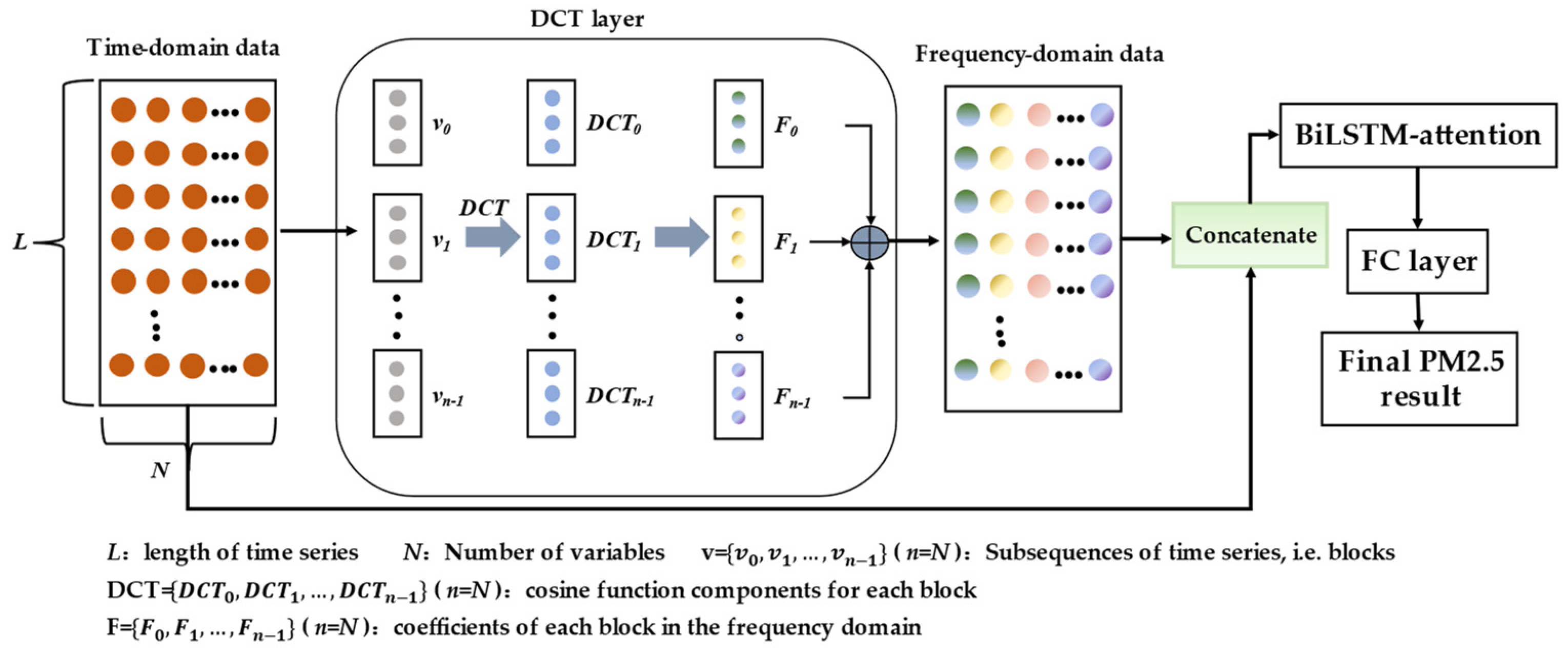
First, it uses DCT to transform the input data from the time domain to the frequency domain. Next, the amalgamation of the time domain dataset with the frequency domain dataset is executed to generate an integrated dataset. This unified dataset is designated as the model’s input, enabling optimal utilization of frequency information while encompassing essential time domain information.

(2)

Adding the attention mechanism after the BiLSTM layer can improve the role of important time steps in BiLSTM, which can in turn improve the prediction effect of the model. Finally, using time frequency domain information, BiLSTM, and attention, it develops the TF-BILSTM-attention model to predict PM2.5 concentration.

(3)

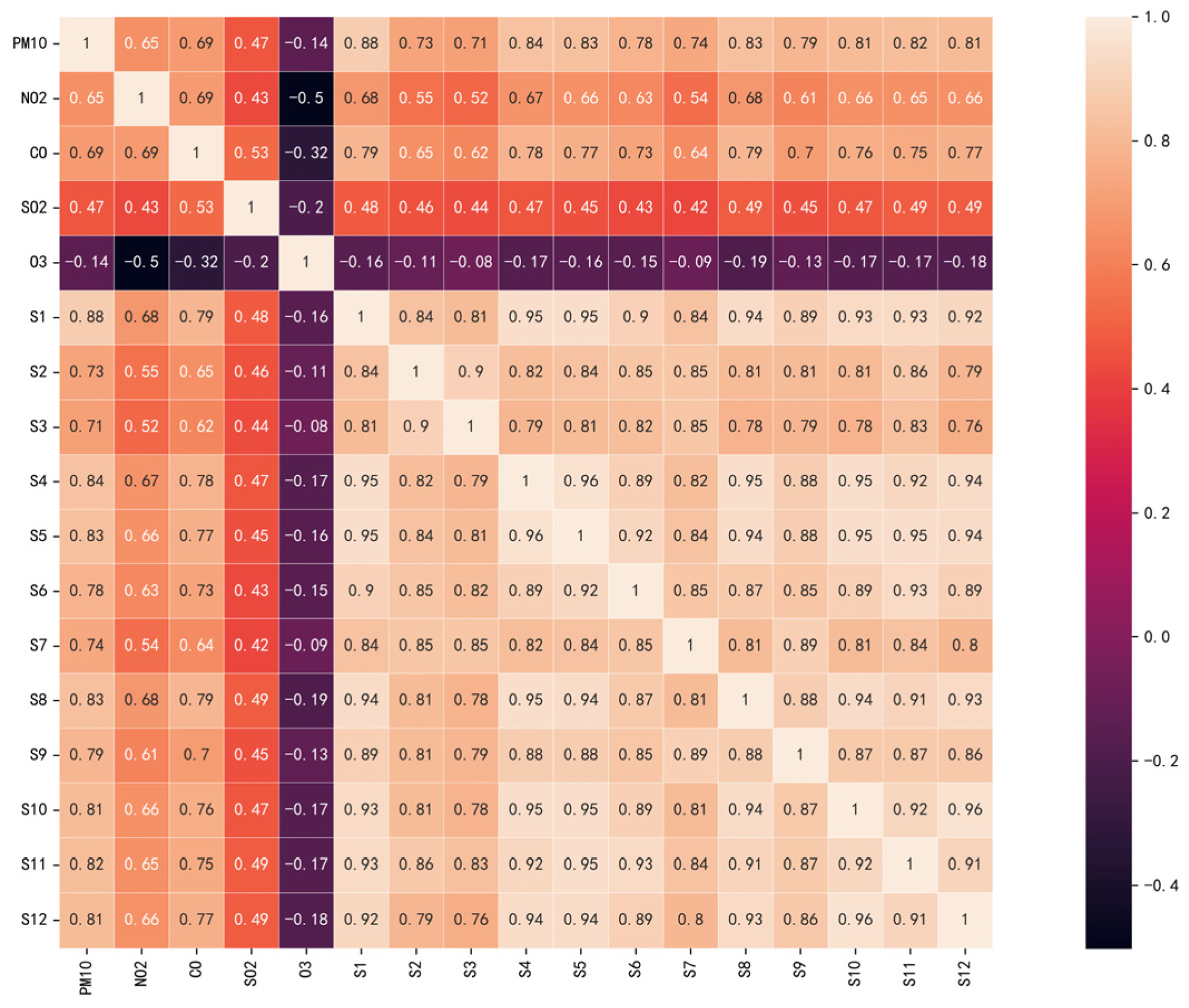
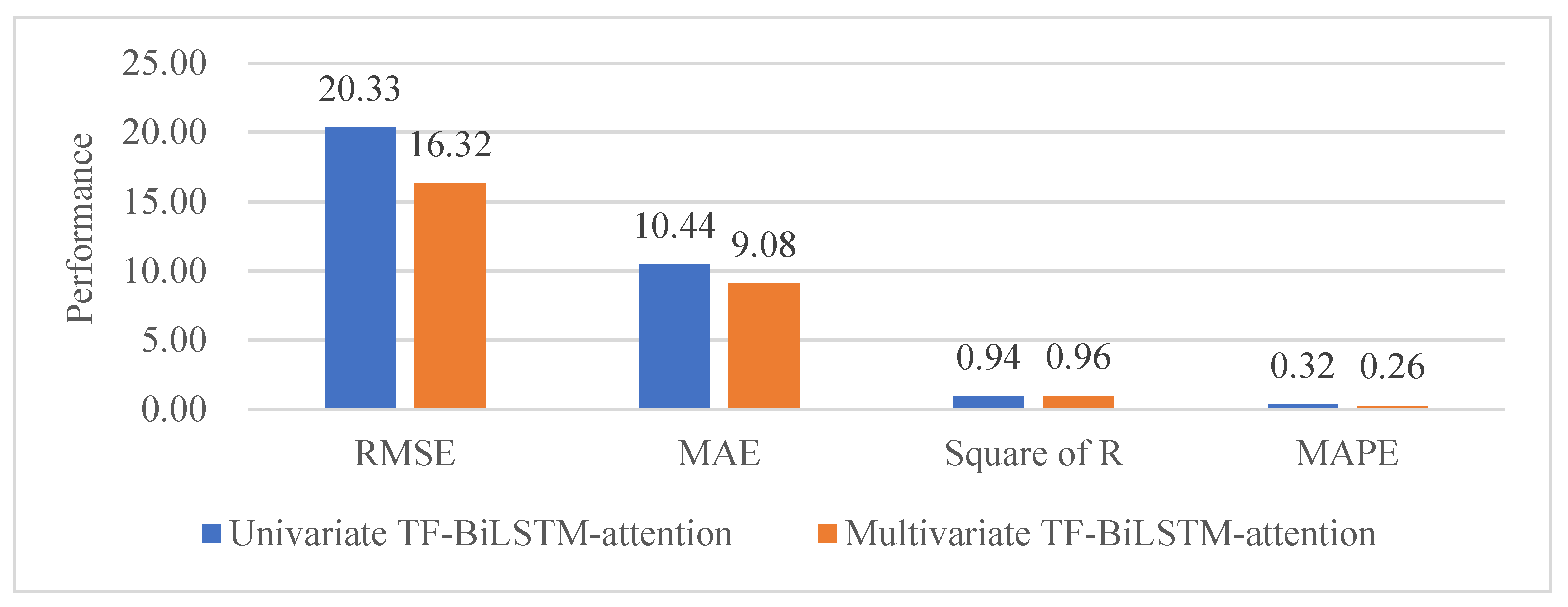
For the multivariate model, the input variables consist solely of the PM2.5 concentration at the site itself and at the remaining 11 sites within the study area, without considering the effects of other pollutant factors and meteorological factors. Empirical findings demonstrate that the multivariate model with these variables added has a good prediction effect.

2. Materials and Methods

2.1. Study Area and Materials

The air quality dataset employed in this study originates from the dataset provided by Zhang et al. [18], which is readily accessible for download from the University of California, Irvine (UCI) Machine Learning Repository page. This dataset encompasses air quality records spanning the period from 2013 to 2017, comprising data collected from 12 distinct Guokong monitoring sites situated in and around Beijing. Specifically, the monitoring sites include Aotizhongxin, Changping, Dingling, Dongsi, Guyuan, Gucheng, Huairou, Nongzhanguan, Shunyi, Tiantan, Wanliu, and Wanshougong. To facilitate the description, we number the above-mentioned sites, with Aotizhongxin noted as S1, Changping as S2, Dingling as S3, and so on.

The individual sites are represented by raw sensor data obtained at hourly intervals, spanning 1461 days with a total of 35,064 data samples. The dataset for each site contains 12 variables. For the purposes of this study, however, only the PM2.5 data series from each site is utilized.

Due to subjective and objective reasons such as instrument damage and human factors [19], there is a certain percentage of missing data in this dataset. Within this study, the missing data are supplied employing the random forest interpolation algorithm [20]. In order to eliminate the different dimensions between the features and speed up the data convergence, we normalize and scale the dataset to [0, 1]. In this case, Equation (1) illustrates the Min-Max normalization method.

$$X=\frac{x-min}{max-min}$$

(1)

where $X$ denotes the normalized value, $x$ denotes the original value, and $min$ and $max$ denote the minimum and maximum values in the dataset, respectively.

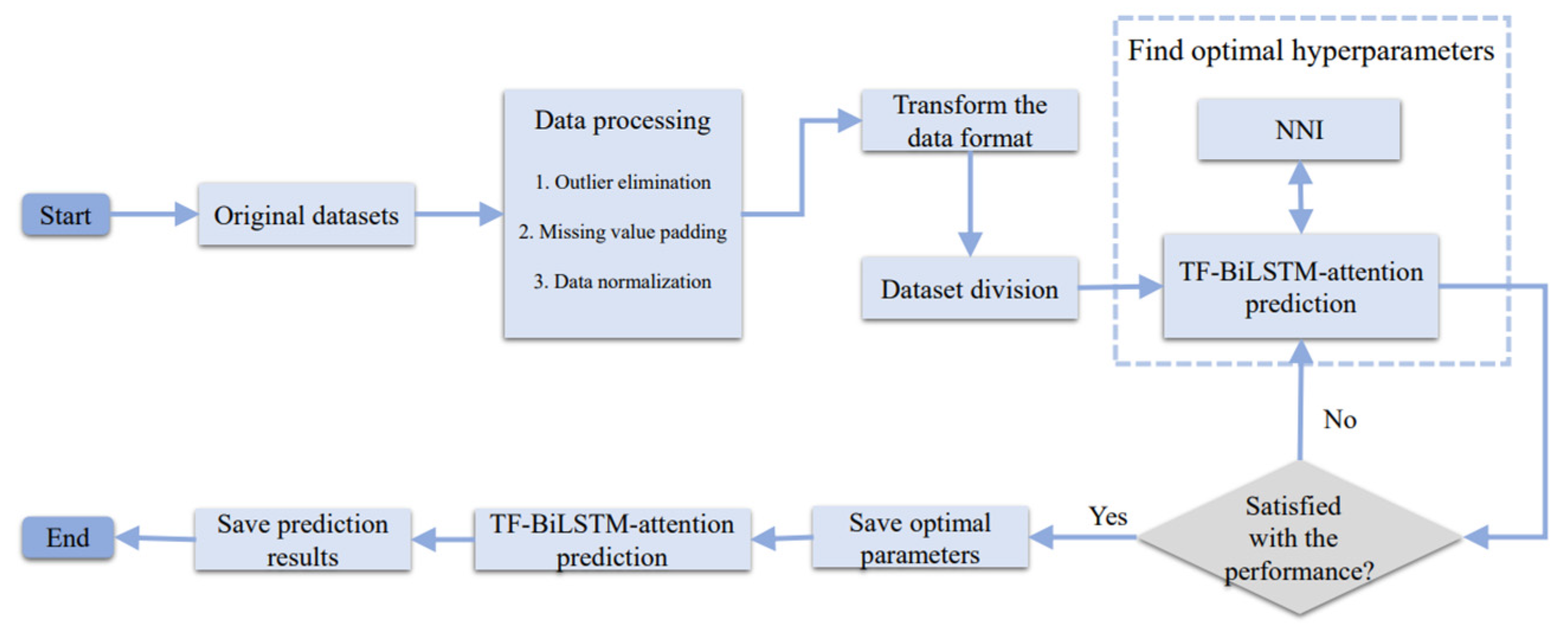
2.2. Methodology Framework

The methodology framework for TF-BiLSTM-attention is depicted in Figure 1, and the detailed training steps for the model are outlined below.

Step 1. Preprocessed data. Firstly, remove the outliers in the original dataset, which include anomalously high or low pollutant concentration values. That is, values that deviate more than three times the standard deviation from the mean pollutant value are removed. Then the corresponding missing data are filled in using the random forest interpolation algorithm. Next, narrow down the data to between 0 and 1 using the Mix–Max normalization algorithm, which speeds up the convergence of the data.

Step 2. Convert the data format. Convert raw multivariate air quality sequences into the supervised learning sequence format. That is, convert the multivariate air quality sequences into a set of sequences containing pairs of inputs and outputs.

Step 3. Divide the dataset. The dataset is partitioned into training and testing sets, with 80% allocated to the training set and the remaining 20% designated for testing purposes.

Step 4. Find optimal hyperparameters and predict the result. Hyperparameters of a model are parameters that are predefined empirically before model training, such as the learning rate, number of iterations, etc. Some researchers in recent years have started to use automatic machine learning (auto-ML) methods to replace manual tuning and thus accomplish hyperparameter optimization. In this paper, the free and open-source Neural Network Intelligence (NNI) framework and the Tree-structured Parzen Estimator (TPE) [21] method are used as the optimization method. The hyperparameter search space of NNI is shown in

Table 1. Search space of Neural Network Intelligence.

Hyperparameters	Search Space
optimizer	{Adam, SGD}
hidden_size of BiLSTM	{1, 2,…, 15}
sequence length	{1, 2,…, 20}
epochs	{5, 10, 15, 20,…, 40}
batch size	{16, 32, 64, 128}
learning rate	{0.1, 0.001, 0.0001}

. Then, the model’s performance is examined on a test dataset to find the optimal hyperparameter combination.

Step 5. Save the prediction model parameters.

2.2.1. Discrete Cosine Transform

The real-world datasets contain rich frequency information and so do the time series datasets. In order to take full advantage of the frequency information in time series data and better determine the hidden data of the series, this paper introduces DCT to turn time domain information into frequency domain information.

DCT is similar to Fourier Transform [13], but DCT achieves better time-frequency energy compression characteristics than Discrete Fourier Transform (DFT), and there is no redundant data in the resultant sequence [13]. Therefore, DCT can extract the frequency information in the time series well.

The DCT of a one-dimensional sequence of length N [22] is defined as

$$\mathrm{F}(u)=c(u){\sum }_{x=0}^{N-1}f\left(x\right)cos\left[\frac{(x+0.5)\pi }{N}u\right]$$

(2)

where $u=0, 1, 2, \dots , N-1$, $\mathrm{F}$ is the transformed sequence, $cos\left[\frac{(x+0.5)\pi }{N}u\right]$ is called forward DCT transformation kernel, $f(·)$ is the original sequence, and $c\left(u\right)$ [22] is a compensation coefficient defined as

$$c(u)=\left\{\begin{array}{c}\sqrt{\frac{1}{N}},u=0\\ \sqrt{\frac{2}{N}},u\ne 0\end{array}\right.$$

(3)

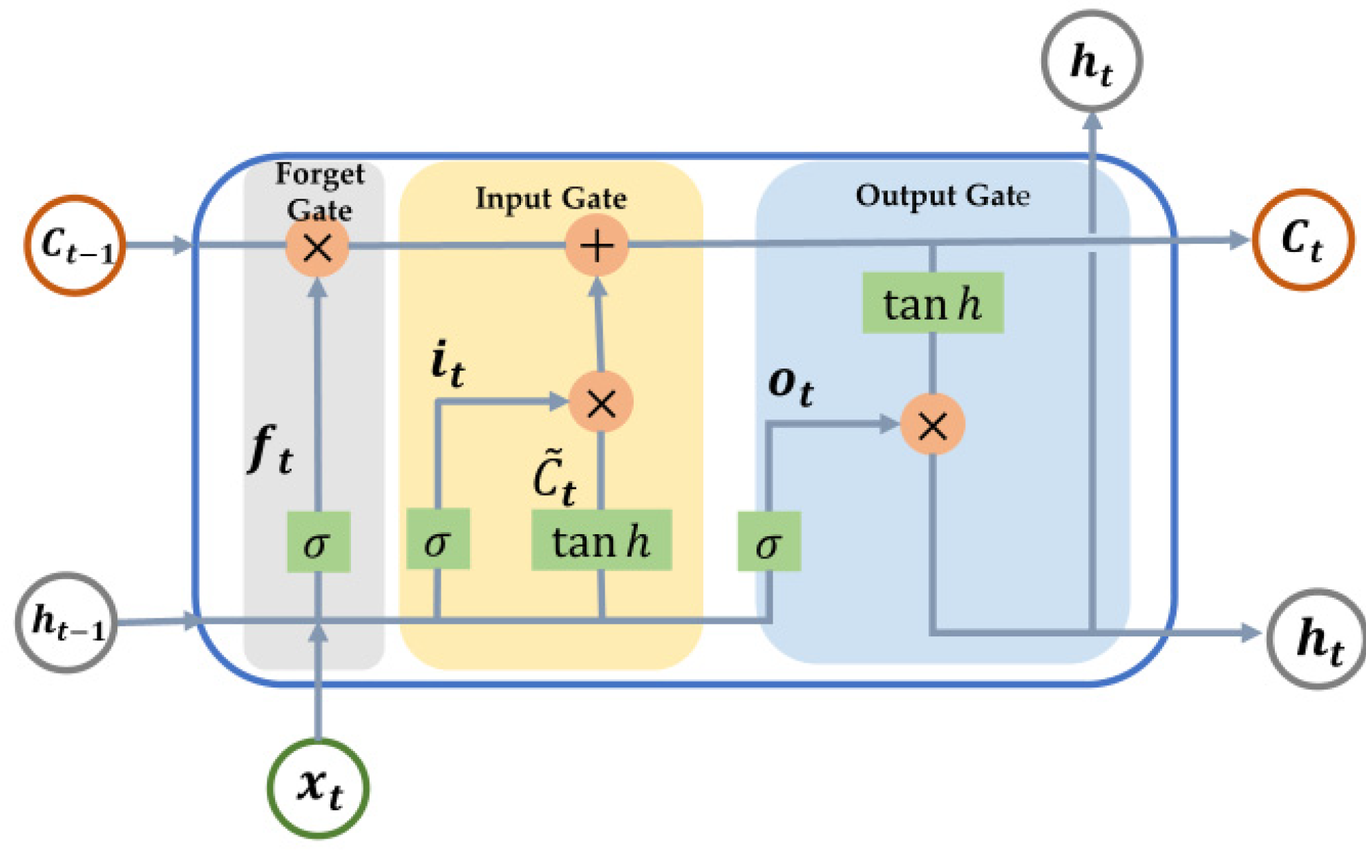
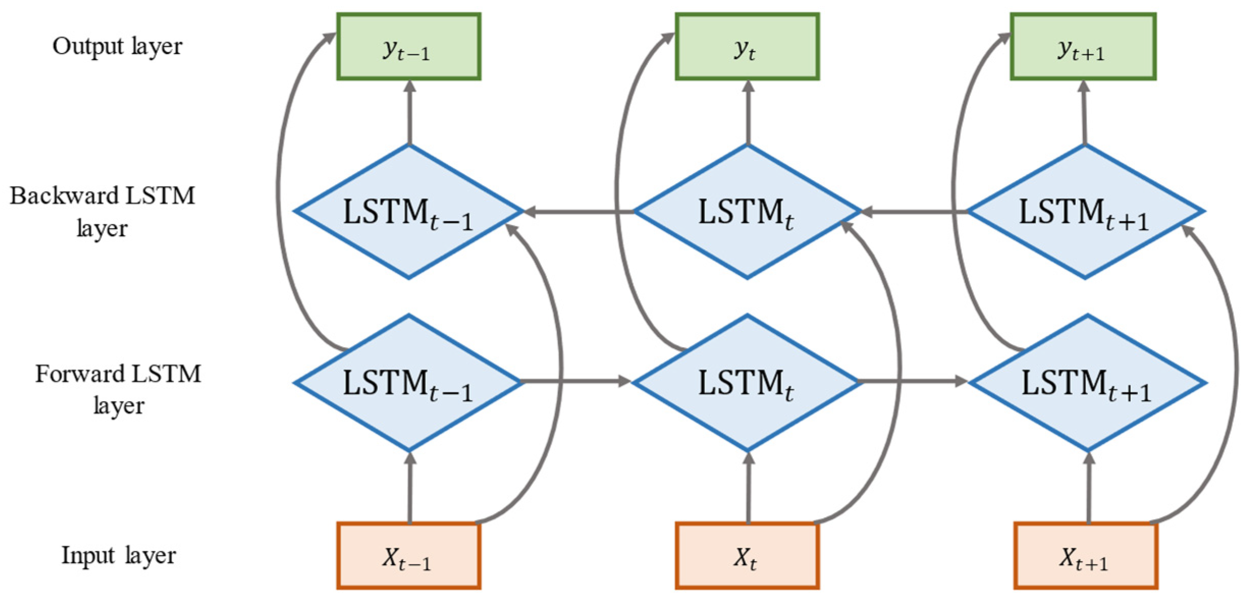
2.2.2. Bidirectional Long Short-Term Memory Neural Network

Long Short-Term Memory Neural Network

LSTM, a type of Recurrent Neural Network (RNN), offers advancements over traditional RNNs by effectively addressing both short-term and long-term dependency issues. Notably, LSTM demonstrates the capability to retain crucial information from early sequences even within lengthy sequences, making it a compelling choice for numerous applications [23]. In recent years, the LSTM neural network is widely used in air quality prediction. Fundamentally, LSTM architecture comprises three pivotal gates: the input gate, forget gate, and output gate, as depicted in Figure 2.

As shown in Figure 2, the inputs and outputs of the network on the LSTM structure are described as follows:

$$f_t=\sigma (W_f·\left[h_{t-1},x_t\right]+b_f)$$

(4)

$$i_t=\sigma (W_i·\left[h_{t-1},x_t\right]+b_i)$$

(5)

$${\tilde{C}}_t=tanh(W_c·\left[h_{t-1},x_t\right]+b_c)$$

(6)

$$C_t=f_t\ast C_{t-1}+i_t\ast {\tilde{C}}_t$$

(7)

$$o_t=\sigma (W_o·\left[h_{t-1},x_t\right]+b_o)$$

(8)

$$h_t=o_t\ast tanh\left(C_t\right)$$

(9)

$$\sigma \left(x\right)=\frac{1}{1+{\mathrm{e}}^{-x}}$$

(10)

$$tanh\left(x\right)=\frac{{\mathrm{e}}^x-{\mathrm{e}}^{-x}}{{\mathrm{e}}^x+{\mathrm{e}}^{-x}}$$

(11)

where $f_t$ represents the forget gate, $i_t$ represents the input gate, ${\tilde{C}}_t$ is a vector created by the $tanh$ layer for the new candidate value,$C_t$ refers to the cell state, $o_t$ represents the output gate, $h_t$ refers to the hidden state, $W_f,W_i$,${ W}_c$ and $W_o$ are input weights, $b_f,b_i,b_c,b_o$ are bias weights, $t$ denotes the current state, and $t-1$ denotes the previous state. $\sigma$ and $\tan h$ are activation functions.

Bidirectional Long Short-Term Memory Neural Network

The BiLSTM model, an extension of the LSTM architecture, comprises two LSTM layers: a forward LSTM layer and a backward LSTM layer. Among them, the forward LSTM processes the sequence in the forward direction and the backward LSTM processes the sequence in the reverse direction, and the outputs of the two LSTMs are spliced together after the processing is completed [11]. Figure 3 presents a schematic representation of the BiLSTM model structure.

As can be seen in Figure 3, BiLSTM can process both forward and backward time series using two LSTMs. Each of these hidden layers in both directions is adept at capturing relevant information from both past and future contexts pertaining to a specific time step. As a result, the features of air pollutants can be extracted more comprehensively using BiLSTM, thus representing an improvement in the predictive performance of the hybrid model.

2.2.3. Attention Mechanism

In the process of time series forecasting, the input features at different times of the time series have different effects on the predicted values, and the smaller the interval from the prediction point, the greater the influence of feature information on the prediction point [16]. The basic BiLSTM network assigns equal weight values to all input features, ignoring the degree of influence of the input features on the predicted values. In this paper, we use the attention mechanism to optimize the basic BiLSTM network, and adding the attention mechanism after the BiLSTM layer can improve the role of important time steps in BiLSTM, which in turn improves the prediction effect of the model.

In this study, the output vectors from the BiLSTM hidden layer serve as inputs to the attention layer, trained by a fully connected layer. The outputs of the fully connected layer are normalized using the softmax function to derive the assigned weights for each hidden layer vector, the size of which indicates the importance of the hidden state for the prediction result at each time step. The weight training process and the weighted average sum of the hidden layer output vectors using the trained weights are described as follows:

$$e_i=tanh(W{k}_i+b)$$

(12)

$$a_i=\frac{exp\left(e_i\right)}{\sum _{j=1}^{T}exp\left(e_j\right)}$$

(13)

$$O_t={\sum }_{i=1}^t{a}_i{k}_i$$

(14)

where $W$ is the weight coefficient and $b$ is the bias coefficient, $k_i$ is the ith hidden unit state value of the output in moment t in the BiLSTM layer. $e_i$ is the score of each hidden unit, $a_i$ is the normalized score, and $O_t$ is the final output of the attention layer.

2.2.4. The TF-BiLSTM-Attention Model

To improve the accuracy of PM2.5 concentration prediction, this study introduces a hybrid model called TF-BiLSTM-attention, integrating the Discrete Cosine Transform [13], BiLSTM [9], and attention mechanism [15]. The model’s framework is visually represented in Figure 4.

Firstly, the data in the time domain are converted into data in the frequency domain by DCT, and then the data in the time domain and the data in the frequency domain are combined to form the input data to be fed into the model. In this way, the model can make use of both time domain and frequency domain information in the prediction process. Next, the long-term and short-term dependencies between the input data are extracted using the BiLSTM network. Then, the prediction results of BiLSTM are obtained, and the attention mechanism is leveraged to assign higher weights to influential factors, thus optimizing resource allocation and elevating prediction accuracy within the model. Finally, the optimized results are put into the output layer and the prediction results are output according to the required dimensions.

2.2.5. Network Architecture and Hyperparameter Setting

The deep neural network in this study is constructed using the PyTorch [24] framework. To determine the optimal performance configuration for the TF-BiLSTM-attention model, experimental investigations are conducted with the assistance of NNI. The final parameter settings that yielded the best results are identified as follows: a hidden size of 11, a sequence length of 7, a batch size of 16, an epoch size of 20, a learning rate of 0.0001, and the adoption of the “adam” optimization function, a widely-used technique in deep neural networks. Moreover, to measure the model’s predictive efficacy, the Mean Squared Error (MSE) loss function is employed, effectively guiding the training process towards attaining accurate predictions.

2.3. Feature Selection

To enhance the predictive accuracy of PM2.5 concentrations, adding pollutant factors and meteorological factors as input features to the model [25] is a common method used by researchers. Considering the spatio-temporal dependence, Wardana et al. [26] analyzed all PM2.5 samples from 12 sites in Beijing and calculated the PM2.5 correlation coefficients between the sites. The experimental results showed that there is a strong correlation of PM2.5 concentration between sites and that adding PM2.5 from other sites as features to the input data can improve the prediction effect of the model. Within this study, we employ the Pearson correlation coefficient [25] to quantify the relationship between the PM2.5 concentration and meteorological features. The formula of the Pearson correlation coefficient is shown in Equation (15).

$${\rho }_{x,y}=\frac{n{\sum }_{i=1}^n{x}_i{y}_i-{\sum }_{i=1}^n{x}_i{\sum }_{i=1}^n{y}_i}{\sqrt{n{\sum }_{i=1}^n{x_i}^2-{({\sum }_{i=1}^n{x}_i)}^2}\sqrt{n{\sum }_{i=1}^n{y_i}^2-{({\sum }_{i=1}^n{y}_i)}^2}}$$

(15)

where x and y denote the input features, and n is the number of samples in the sequence.

Figure 5 shows a heat map of the correlation coefficients between the six pollutants at site S1 itself and a total of 17 features of PM2.5 concentration at the remaining 11 sites, where S1, S2, S3, S4, etc. represent the PM2.5 concentration of each site, respectively. As can be seen in Figure 5, the correlations of the six pollutant factors at site S1 vary considerably, with the PM2.5 concentration at site S1 having the highest correlation with the PM10 concentration at its own site, and the lowest correlation with the O3 concentration at its own site. In contrast, the concentrations of PM2.5 at all 12 sites are strongly correlated with each other (ρ > 0.7). The observed strong correlation indicates a substantial spatial dependence concerning PM2.5 levels among the various monitoring sites.

Meanwhile, Wardana et al. [26] conducted comparative experiments using different input variables. The findings demonstrated that, for the same model, the prediction effect of using the PM2.5 concentration at this site and the PM2.5 concentration at other sites as the input variables was better than the prediction effect of the model using the pollutant factors and meteorological factors at this site as the input variables. Therefore, in this paper, only the PM2.5 concentration at this site and the PM2.5 concentration at other sites are also used as input variables for the multivariate model without considering other pollutant factors and meteorological factors.

2.4. Evaluation of Prediction Results

In order to assess the predictive accuracy of the model, we chose mean absolute error (MAE), root mean square error (RMSE), average absolute percentage error (MAPE), and coefficient of determination (R²) as model evaluation metrics. The calculations are shown in Equations (16)–(19).

$$\mathrm{MAE}=\frac{1}{n}{\sum }_{i=1}^n|y_i-\widehat{y_i}|$$

(16)

$$\mathrm{RMSE}=\sqrt{\frac{1}{n}{\sum }_{i=1}^n{\left(y_i-\widehat{y_i}\right)}^2}$$

(17)

$$\mathrm{MAPE}=\frac{1}{n}{\sum }_{i=1}^n\frac{|y_i-\widehat{y_i}|}{y_i}$$

(18)

$${\mathrm{R}}^2=1-\frac{{\sum }_{i=1}^n{\left(y_i-\widehat{y_i}\right)}^2}{{\sum }_{i=1}^n{\left(y_i-\overline{y_i}\right)}^2}$$

(19)

where $y_i$ denotes the true value, $\widehat{y_i}$ denotes the predicted value, and $\overline{y_i}$ denotes the mean of all true values.

Lower values of MAE, RMSE, and MAPE indicate diminished error levels, implying more accurate predictions. Meanwhile, as the R² value gets closer to 1, the better the model is fitted.

3. Results

To validate the effectiveness of our proposed model, a series of experiments is conducted. First, only use the variable PM2.5 at this site as an input to the model. Specifically, we compare four models using a single variable, including BiLSTM, BiLSTM-attention, TF-BiLSTM, and TF-BiLSTM-attention. Second, a total of 12 variables, including the PM2.5 concentration at this site and the PM2.5 concentrations at the remaining 11 sites in the study area, are used as inputs to the model. Our proposed univariate model is first compared with the multivariate model, and then the multivariate model is compared with other basic multivariate models and hybrid multivariate models.

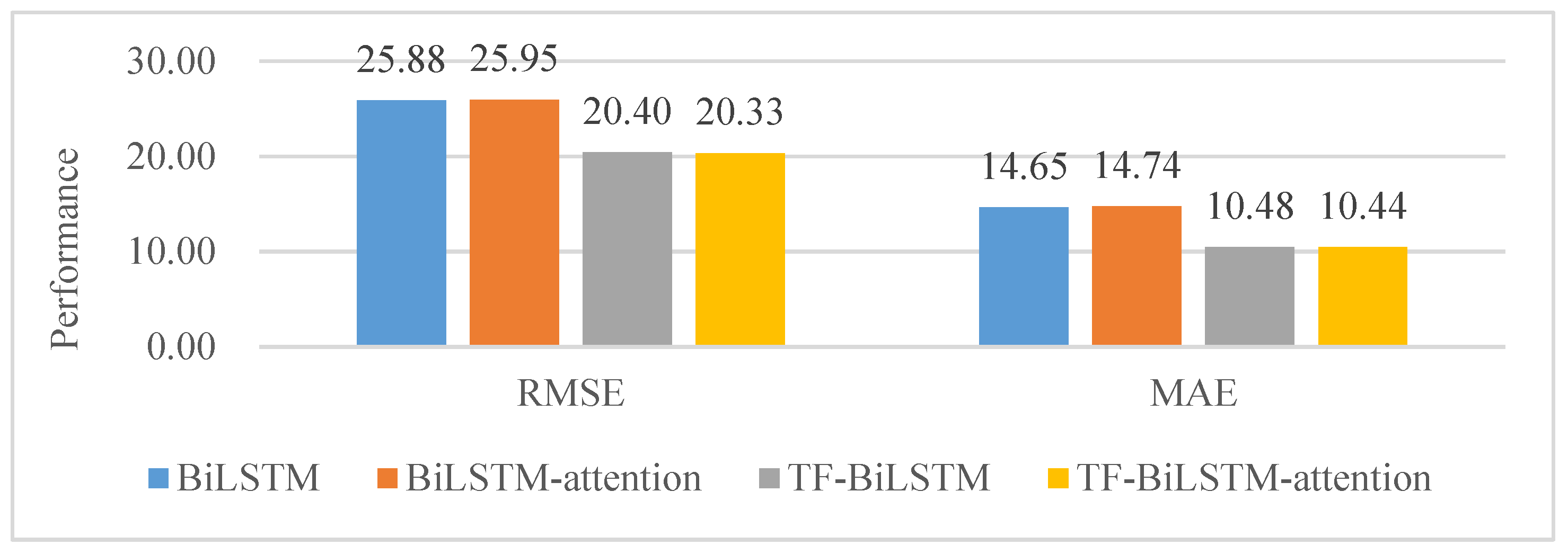
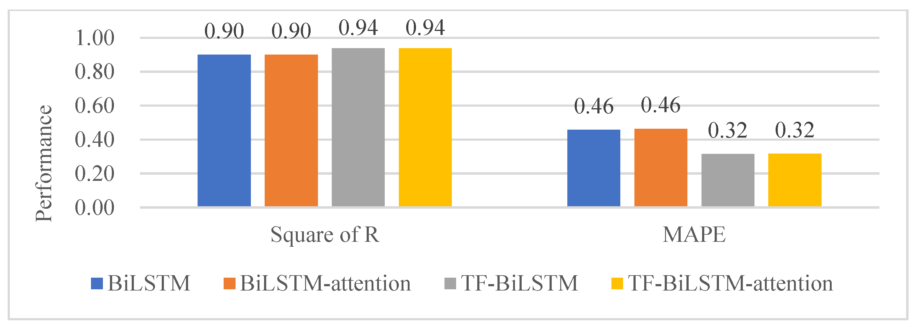
3.1. Comparison with Different Univariate Models

Table 2. Comparison of different models using PM2.5 as the input in terms of RMSE, MAE, R², and MAPE.

		S1	S2	S3	S4	S5	S6	S7	S8	S9	S10	S11	S12	Mean
RMSE	BiLSTM	25.7021	23.8906	21.1004	28.3287	26.4759	28.4701	22.4960	27.7977	27.5000	25.0629	25.2665	28.4127	25.8753
	BiLSTM-attention	25.7708	24.0441	21.4432	28.3129	26.4545	28.3707	22.5573	27.8118	27.6883	25.0518	25.2951	28.6464	25.9539
	TF-BiLSTM	19.1547	19.7329	17.8799	21.8664	20.4544	21.4437	18.8393	22.0770	20.6508	18.9912	19.8951	23.8156	20.4001
	TF-BiLSTM-attention	19.0154	19.9404	17.8012	21.6904	20.4426	21.4567	18.7613	21.9312	20.4372	18.9155	19.8894	23.7143	20.3330
MAE	BiLSTM	14.9132	13.5171	11.7857	16.2541	15.4316	15.8921	11.7416	15.8277	15.4688	14.7648	14.2116	15.9601	14.6474
	BiLSTM-attention	14.9621	13.5376	11.9318	16.3292	15.4384	15.8559	11.8141	15.9874	15.7161	14.8636	14.2167	16.1878	14.7367
	TF-BiLSTM	10.3375	10.3115	9.3581	11.1289	11.0317	10.7332	8.7072	11.1015	10.5434	10.6783	10.0862	11.7263	10.4787
	TF-BiLSTM-attention	10.2423	10.3312	9.3309	10.9785	11.0520	10.7917	8.6934	10.9732	10.4370	10.6395	10.1646	11.6934	10.4440
R2	BiLSTM	0.9052	0.8916	0.8966	0.9035	0.9075	0.8988	0.8930	0.9004	0.8869	0.9115	0.9041	0.9048	0.9003
	BiLSTM-attention	0.9047	0.8902	0.8933	0.9036	0.9077	0.8996	0.8924	0.9003	0.8854	0.9116	0.9039	0.9032	0.8996
	TF-BiLSTM	0.9473	0.9261	0.9258	0.9425	0.9448	0.9426	0.9249	0.9372	0.9362	0.9492	0.9405	0.9331	0.9375
	TF-BiLSTM-attention	0.9481	0.9245	0.9264	0.9434	0.9449	0.9425	0.9256	0.9380	0.9376	0.9496	0.9406	0.9337	0.9379
MAPE	BiLSTM	0.4400	0.4512	0.5211	0.4775	0.4393	0.4192	0.4630	0.4646	0.4818	0.4321	0.4454	0.4549	0.4575
	BiLSTM-attention	0.4463	0.4429	0.5183	0.4830	0.4425	0.4209	0.4659	0.4795	0.5054	0.4481	0.4375	0.4688	0.4632
	TF-BiLSTM	0.2899	0.3227	0.4234	0.3270	0.2868	0.2482	0.3479	0.3039	0.3057	0.3124	0.2937	0.3283	0.3158
	TF-BiLSTM-attention	0.2850	0.3289	0.4278	0.3240	0.2876	0.2510	0.3465	0.2920	0.2985	0.3204	0.2963	0.3397	0.3165

demonstrates the comparison between the four models using univariate inputs for each site. A comparison of the overall predictive effectiveness of the four univariate models for the 12 sites is shown in Figure 6 and Figure 7. Figure 6 and Figure 7 illustrate that the TF-BiLSTM-attention model for the 12 sites has the smallest mean value of RMSE and the mean value of MAE, and the mean value of R² is the largest. This indicates that the TF-BiLSTM-attention model performs the best among the four models. The difference of the forecast effect between the TF-BiLSTM model and the TF-BiLSTM-attention model is very small. The difference of the forecast effect between the BiLSTM model and the BiLSTM-attention model is also very small. However, incorporating the attention mechanism renders an improvement over the model lacking this feature, which indicates that in the case of univariate input, the attention mechanism does not improve the prediction effect of the model significantly. Finally, the prediction effect of the TF-BiLSTM model is significantly better than that of the BiLSTM model, which indicates that adding frequency information to the model can improve the prediction effect of the model. Meanwhile, it can be found from Table 2 that the same model has different prediction effects for different sites. Taking the univariate TF-BiLSTM-attention model, which has the best performance in general, as an example, site S12 has the worst performance, site S3 has the smallest value of RMSE, site S7 has the smallest value of MAE, site S10 has the largest value of R², and site S6 has the smallest value of MAPE.

3.2. Comparison with Different Multivariate Models

In this study, we take the PM2.5 concentration at its own site and the PM2.5 concentration at 11 other sites as the input variables of the multivariate model. The prediction effects of the univariate TF-BiLSTM-attention and multivariate TF-BiLSTM-attention models are shown in Figure 8. Figure 8 illustrates that the multivariate model provides significantly better prediction performance compared to the univariate model. This suggests that incorporating the PM2.5 concentration data from the remaining 11 sites as input variables enhances the predictive capability of the model.

For this study, we select four basic models, LSTM, BiLSTM, Gate Recurrent Unit (GRU), and Bidirectional Gate Recurrent Unit (BiGRU), and four hybrid models, CNN-LSTM, CNN-BiLSTM, CNN-GRU, and CNN-BiGRU, to compare with our proposed models. Also, two models, TF- BiLSTM and TF-CNN-BiLSTM, are constructed to compare with our proposed models. The prediction performances of different multivariate models are shown in

Table 3. Comparison of RMSE, MAE of different multivariate models.

		S1	S2	S3	S4	S5	S6	S7	S8	S9	S10	S11	S12	Mean
RMSE	LSTM	18.1006	19.2394	17.4561	21.1559	19.5055	21.6548	18.1532	20.5995	21.0374	19.3954	18.4665	23.2015	19.8305
	BiLSTM	18.0737	19.5708	17.4851	21.5529	19.5199	21.5024	18.2051	20.6116	21.0968	20.0648	18.5075	23.2385	19.9524
	GRU	18.2846	19.5202	17.4705	21.3097	19.5682	21.7809	18.3439	20.6879	20.9501	19.7772	18.7310	23.3706	19.9829
	BiGRU	18.4066	19.5196	17.5263	21.4471	19.7659	21.8864	18.3044	20.6079	21.1133	19.8293	18.9517	23.6979	20.0880
	CNN-LSTM	18.3998	19.7535	17.5423	21.9600	20.0875	21.7654	18.2582	21.3936	21.3831	20.5814	18.4875	23.5033	20.2596
	CNN-BiLSTM	18.0460	19.5669	17.5357	21.5193	20.0994	21.8662	18.1882	21.4694	21.0171	21.1142	18.6094	23.1787	20.1842
	CNN-GRU	18.2183	19.6874	17.5565	21.8348	19.7397	22.0151	18.2250	20.8662	20.7810	20.0161	18.5489	23.4618	20.0792
	CNN-BiGRU	18.2668	19.7464	17.5711	21.6076	19.9810	22.1604	18.3079	20.7632	21.0255	20.2230	18.5808	18.5808	19.7345
	TF-BiLSTM	16.1178	17.3627	15.8417	19.8267	17.8521	18.6915	16.7548	18.1906	17.6451	17.3203	17.1758	20.8809	17.8050
	TF-CNN-BiLSTM	17.9947	19.8441	17.4662	21.8841	19.6320	22.0485	18.4108	20.6858	20.7671	20.3364	18.5153	23.6375	20.1019
	TF-BiLSTM-attention	15.1313	14.8985	13.9907	19.2926	17.1282	16.9033	15.1524	17.4800	16.6834	16.0785	15.6039	17.5039	16.3205
MAE	LSTM	10.2881	10.8300	9.0488	12.0672	10.8458	11.2159	9.1468	11.0433	11.5139	11.5522	9.9805	12.1749	10.8089
	BiLSTM	10.2844	10.9388	9.1592	12.6651	10.8806	11.3226	9.2960	11.0438	11.6228	12.2251	10.0081	12.1888	10.9696
	GRU	10.5620	11.1118	9.0461	12.3556	10.8661	11.5645	9.4594	11.1828	11.4348	11.6418	10.0806	12.2258	10.9609
	BiGRU	10.5188	10.9987	9.0619	12.2387	10.9713	11.5515	9.3846	11.0888	11.5483	11.6911	10.1389	12.3704	10.9636
	CNN-LSTM	10.4881	11.2544	8.9708	13.2826	11.2823	11.5292	9.3826	11.6358	12.0585	12.6506	10.1415	12.3071	11.2486
	CNN-BiLSTM	10.2668	11.0377	9.0081	12.7124	11.1819	11.4192	9.3518	11.7242	11.5822	13.1375	10.2952	12.1018	11.1516
	CNN-GRU	10.4272	11.0820	8.9467	13.2888	10.9788	11.5129	9.3631	11.0701	11.2701	11.8321	9.9739	12.2517	10.9998
	CNN-BiGRU	10.3830	11.2317	8.9172	12.8078	11.1421	11.6240	9.2699	10.9867	11.4748	11.8551	9.9910	9.9910	10.8062
	TF-BiLSTM	8.9259	9.0709	8.2499	11.3809	9.7360	9.6060	8.2254	9.4048	9.7731	11.2918	9.6746	10.5580	9.6581
	TF-CNN-BiLSTM	10.1281	10.8575	9.0618	13.1646	10.8501	11.4350	9.5689	11.0274	11.5016	12.2689	10.0571	12.3003	11.0184
	TF-BiLSTM-attention	8.7559	8.1511	7.3247	10.8909	9.7660	9.0983	7.2614	8.9792	9.7707	11.0173	8.8407	9.1302	9.0822

and

Table 4. Comparison of R², MAPE of different multivariate models.

		S1	S2	S3	S4	S5	S6	S7	S8	S9	S10	S11	S12	Mean
R2	LSTM	0.9530	0.9297	0.9293	0.9462	0.9498	0.9415	0.9303	0.9453	0.9338	0.9470	0.9488	0.9365	0.9409
	BiLSTM	0.9531	0.9273	0.9290	0.9442	0.9497	0.9423	0.9299	0.9452	0.9335	0.9433	0.9485	0.9363	0.9402
	GRU	0.9520	0.9276	0.9291	0.9454	0.9495	0.9408	0.9288	0.9448	0.9344	0.9449	0.9473	0.9356	0.9400
	BiGRU	0.9514	0.9276	0.9287	0.9447	0.9485	0.9402	0.9291	0.9453	0.9334	0.9446	0.9460	0.9337	0.9394
	CNN-LSTM	0.9522	0.9259	0.9286	0.9420	0.9468	0.9409	0.9295	0.9410	0.9316	0.9403	0.9486	0.9348	0.9385
	CNN-BiLSTM	0.9533	0.9273	0.9286	0.9443	0.9467	0.9403	0.9300	0.9406	0.9340	0.9372	0.9480	0.9366	0.9389
	CNN-GRU	0.9524	0.9264	0.9284	0.9427	0.9486	0.9395	0.9298	0.9439	0.9354	0.9435	0.9483	0.9351	0.9395
	CNN-BiGRU	0.9521	0.9260	0.9283	0.9439	0.9473	0.9387	0.9291	0.9444	0.9339	0.9424	0.9481	0.9481	0.9402
	TF-BiLSTM	0.9627	0.9428	0.9417	0.9527	0.9580	0.9564	0.9406	0.9573	0.9535	0.9577	0.9557	0.9486	0.9523
	TF-CNN-BiLSTM	0.9535	0.9252	0.9292	0.9424	0.9491	0.9393	0.9283	0.9448	0.9355	0.9417	0.9485	0.9341	0.9393
	TF-BiLSTM-attention	0.9671	0.9579	0.9546	0.9553	0.9613	0.9643	0.9514	0.9606	0.9584	0.9636	0.9634	0.9639	0.9601
MAPE	LSTM	0.3097	0.3697	0.3620	0.4138	0.2948	0.2795	0.3524	0.2875	0.2745	0.2780	0.2737	0.3005	0.3163
	BiLSTM	0.2985	0.3743	0.3769	0.4474	0.2916	0.2889	0.3714	0.2896	0.2800	0.2870	0.2679	0.2994	0.3227
	GRU	0.3397	0.3932	0.3519	0.4250	0.3002	0.3145	0.3899	0.3124	0.2825	0.2828	0.2894	0.3168	0.3332
	BiGRU	0.3357	0.3847	0.3594	0.4142	0.3137	0.3130	0.3814	0.3178	0.2822	0.2801	0.2849	0.3103	0.3315
	CNN-LSTM	0.3301	0.4054	0.3280	0.4645	0.3114	0.3072	0.3746	0.2873	0.2864	0.2979	0.2614	0.3088	0.3303
	CNN-BiLSTM	0.3087	0.3866	0.3387	0.4533	0.3030	0.2905	0.3677	0.2855	0.2796	0.3008	0.2597	0.3155	0.3241
	CNN-GRU	0.3270	0.3889	0.3213	0.4807	0.2903	0.2956	0.3728	0.2932	0.2789	0.2821	0.2667	0.3270	0.3270
	CNN-BiGRU	0.3229	0.4047	0.3151	0.4420	0.3071	0.2985	0.3516	0.2865	0.2792	0.2836	0.2801	0.2801	0.3210
	TF-BiLSTM	0.2463	0.2889	0.3538	0.3612	0.2567	0.2090	0.3121	0.2426	0.2542	0.3036	0.2470	0.2694	0.2787
	TF-CNN-BiLSTM	0.3094	0.3586	0.3686	0.4758	0.3060	0.2687	0.3894	0.3093	0.2741	0.2890	0.2792	0.3148	0.3286
	TF-BiLSTM-attention	0.2365	0.2253	0.2675	0.3375	0.2489	0.1947	0.2728	0.2382	0.2729	0.2736	0.2373	0.2696	0.2562

. Table 3 and Table 4 provide a clear depiction, illustrating that the mean value of RMSE, the mean value of MAE, and the mean value of MAPE are the smallest, and the mean value of R² is the largest for the 12 sites of our proposed model. This indicates that the TF-BiLSTM-attention model has the best prediction performance among these multivariate models.

From a single site, the values of the evaluation metrics of the multivariate LSTM, BiLSTM, GRU, and BiGRU models do not differ much from each other, which suggests that under the same conditions, the prediction effect of these four models is about the same. Meanwhile, the difference in the values of the evaluation metrics between the hybrid model with the CNN network added and the base model is also not significant, which indicates that adding a layer of 1D-CNN to a single base model in this study does not significantly improve the prediction effect of the model.

From the overall effect of the 12 sites, when the three multivariate models, TF-BiLSTM, TF-CNN-BiLSTM, and TF-BiLSTM-attention, are compared with each other, the TF-BiLSTM-attention model has the best prediction effect, the TF- BiLSTM model is the second best, and the TF-CNN-BiLSTM model is the worst. This indicates that after adding the frequency domain information in the model, the feature information cannot be better extracted using the CNN network. Instead, adding the attention mechanism in the model can play a role in improving the prediction effect of the model. Meanwhile, compared with the univariate model, the multivariate model with the addition of the attention mechanism has a higher degree of improvement in the prediction effect than that of the univariate model.

4. Conclusions

In this paper, we propose the TF-BiLSTM-attention model for PM2.5 concentration prediction at 12 sites in Beijing. In order to capture the frequency information in the PM2.5 concentration series, firstly, the DCT is used to transform the time domain series into the frequency domain series. Secondly, the original time domain series is united with the frequency domain series, allowing the model to effectively utilize both the time and frequency domain information. The input features at different times of the time series have different effects on the predicted values, while the basic BiLSTM network assigns equal weight values to all the input features, ignoring the degree of influence of the input features on the predicted values. For this reason, we add the attention mechanism after the BiLSTM network to give higher weights to the factors with higher influence. At the same time, taking advantage of the high spatial dependence of PM2.5 concentration data from different sites, a total of 12 variables, including the PM2.5 concentration at its own site and that of the remaining 11 sites in the study area, are used as input variables for the multivariate model. The results demonstrate superior prediction performance of the model incorporating frequency domain information compared to the model solely utilizing time domain information. Furthermore, the hybrid model augmented with the attention mechanism outperforms the hybrid model without this augmentation. Our proposed TF-BiLSTM-attention model outperforms all the basic and hybrid models in the experiment. The improved model will be able to capture key information and trends in the time series data more accurately. This will help to improve the accurate prediction of pollutant concentrations, meteorological conditions, and other factors, thus improving the overall prediction accuracy. Nevertheless, using DCT and adding the attention mechanism to the base BiLSTM model results in a model with higher complexity. It takes longer time to train a complex model, and the longer computation time may affect the real-time availability of air quality predictions, making it more difficult to update and provide information in a timely manner. Therefore, in future applications, we will strive to find a suitable balance between model complexity and computational efficiency. In addition, this study is limited by the lack of spatial feature information related to PM2.5 to explain the generalization of the model to different regions. For this reason, a large amount of real and valid air quality related data will be collected in the future, and the model proposed in this paper will be applied to several datasets from different regions for validation.

References

1. Fan, H.; Zhao, C.; Yang, Y. A comprehensive analysis of the spatio-temporal variation of urban air pollution in China during 2014–2018. Atmos. Environ. 2020, 220, 117066. [Google Scholar] [CrossRef]
2. Lin, Y.C.; Lee, S.J.; Ouyang, C.S.; Wu, C.H. Air quality prediction by neuro-fuzzy modeling approach. Appl. Soft Comput. 2020, 86, 105898. [Google Scholar] [CrossRef]
3. Gu, K.; Zhou, Y.; Sun, H.; Zhao, L.; Liu, S. Prediction of air quality in Shenzhen based on neural network algorithm. Neural Comput. Appl. 2020, 32, 1879–1892. [Google Scholar] [CrossRef]
4. Mengfan, T.; Siwei, L.; Lechao, D.; Senlin, H. Including the feature of appropriate adjacent sites improves the PM2.5 concentration prediction with long short-term memory neural network model. Sustain. Cities Soc. 2022, 76, 103427. [Google Scholar] [CrossRef]
5. Pak, U.; Ma, J.; Ryu, U.; Ryom, K.; Juhyok, U.; Pak, K.; Pak, C. Deep learning-based PM2.5 prediction considering the spatiotemporal correlations: A case study of Beijing, China. Sci. Total Environ. 2020, 699, 133561. [Google Scholar] [CrossRef] [PubMed]
6. Chang-Hoi, H.; Park, I.; Oh, H.R.; Gim, H.J.; Hur, S.K.; Kim, J.; Choi, D.R. Development of a PM2.5 prediction model using a recurrent neural network algorithm for the Seoul metropolitan area, Republic of Korea. Atmos. Environ. 2021, 245, 118021. [Google Scholar] [CrossRef]
7. Jiang, P.; Dong, Q.; Li, P. A novel hybrid strategy for PM2.5 concentration analysis and prediction. J. Environ. Manag. 2017, 196, 443–457. [Google Scholar] [CrossRef]
8. Hua, Y.; Zhao, Z.; Li, R.; Chen, X.; Liu, Z.; Zhang, H. Deep learning with long short-term memory for time series prediction. IEEE Commun. Mag. 2019, 57, 114–119. [Google Scholar] [CrossRef]
9. Prihatno, A.T.; Nurcahyanto, H.; Ahmed, M.F.; Rahman, M.H.; Alam, M.M.; Jang, Y.M. Forecasting PM2.5 concentration using a single-dense layer BiLSTM method. Electronics 2021, 10, 1808. [Google Scholar] [CrossRef]
10. Li, T.; Hua, M.; Wu, X.U. A hybrid CNN-LSTM model for forecasting particulate matter (PM2.5). IEEE Access 2020, 8, 26933–26940. [Google Scholar] [CrossRef]
11. Zhang, C.; Ma, H.; Hua, L.; Sun, W.; Nazir, M.S.; Peng, T. An evolutionary deep learning model based on TVFEMD, improved sine cosine algorithm, CNN and BiLSTM for wind speed prediction. Energy 2022, 254, 124250. [Google Scholar] [CrossRef]
12. Zhu, M.; Xie, J. Investigation of nearby monitoring station for hourly PM2.5 forecasting using parallel multi-input 1D-CNN-biLSTM. Expert Syst. Appl. 2023, 211, 118707. [Google Scholar] [CrossRef]
13. Jiang, M.; Zeng, P.; Wang, K.; Liu, H.; Chen, W.; Liu, H. FECAM: Frequency enhanced channel attention mechanism for time series forecasting. Adv. Eng. Inform. 2023, 58, 102158. [Google Scholar] [CrossRef]
14. Chen, Y.; Liu, S.; Yang, J.; Jing, H.; Zhao, W.; Yang, G. A Joint Time-frequency Domain Transformer for Multivariate Time Series Forecasting. arXiv 2023, arXiv:2305.14649. [Google Scholar]
15. Niu, Z.; Zhong, G.; Yu, H. A review on the attention mechanism of deep learning. Neurocomputing 2021, 452, 48–62. [Google Scholar] [CrossRef]
16. Zhou, H.; Wang, T.; Zhao, H.; Wang, Z. Updated Prediction of Air Quality Based on Kalman-Attention-LSTM Network. Sustainability 2022, 15, 356. [Google Scholar] [CrossRef]
17. Wang, J.; Li, J.; Wang, X.; Wang, T.; Sun, Q. An quality prediction model based on CNN-BiNLSTM-attention. Environ. Dev. Sustain. 2022, 12, 1–16. [Google Scholar] [CrossRef]
18. Zhang, S.; Guo, B.; Dong, A.; He, J.; Xu, Z.; Chen, S.X. Cautionary tales on air-quality improvement in Beijing. Proc. R. Soc. A 2017, 473, 20170457. [Google Scholar] [CrossRef]
19. Chen, X.; Sun, L. Bayesian temporal factorization for multidimensional time series prediction. IEEE Trans. Pattern Anal. Mach. Intell. 2021, 44, 4659–4673. [Google Scholar] [CrossRef]
20. Alsaber, A.R.; Pan, J.; Al-Hurban, A. Handling complex missing data using random forest approach for an air quality monitoring dataset: A case study of Kuwait environmental data (2012 to 2018). Int. J. Environ. Res. Public Health 2021, 18, 1333. [Google Scholar] [CrossRef]
21. Li, W.; Ding, P.; Xia, W.; Chen, S.; Yu, F.; Duan, C.; Cui, D.; Chen, C. Artificial neural network reconstructs core power distribution. Nucl. Eng. Technol. 2022, 54, 617–626. [Google Scholar] [CrossRef]
22. Bi, X.; Zhang, C.; He, Y.; Zhao, X.; Sun, Y.; Ma, Y. Explainable time–frequency convolutional neural network for microseismic waveform classification. Inf. Sci. 2021, 546, 883–896. [Google Scholar] [CrossRef]
23. Akilandeswari, P.; Manoranjitham, T.; Kalaivani, J.; Nagarajan, G. Air quality prediction for sustainable development using LSTM with weighted distance grey wolf optimizer. Soft Comput. 2023, 1–10. [Google Scholar] [CrossRef]
24. Paszke, A.; Gross, S.; Massa, F.; Lerer, A.; Bradbury, J.; Chanan, G.; Killeen, T.; Lin, Z.; Gimelshein, N.; Antiga, L.; et al. Pytorch: An imperative style, high-performance deep learning library. Adv. Neural Inf. Process. Syst. 2019, 32, 8024–8035. [Google Scholar]
25. Huang, G.; Li, X.; Zhang, B.; Ren, J. PM2.5 concentration forecasting at surface monitoring sites using GRU neural network based on empirical mode decomposition. Sci. Total Environ. 2021, 768, 144516. [Google Scholar] [CrossRef]
26. Wardana, I.N.K.; Gardner, J.W.; Fahmy, S.A. Optimising deep learning at the edge for accurate hourly air quality prediction. Sensors 2021, 21, 1064. [Google Scholar] [CrossRef]
Figure 1. Methodology framework of this study.
Applsci 13 12794 g001
Figure 2. Structure of LSTM.
Applsci 13 12794 g002
Figure 3. Structure of the BiLSTM network.
Applsci 13 12794 g003
Figure 4. The framework of TF-BiLSTM-attention model.
Applsci 13 12794 g004
Figure 5. Heat map of correlation coefficients between different features of site S1.
Applsci 13 12794 g005
Figure 6. Comparison of mean values of RMSE and MAE for 12 sites with different univariate models.
Applsci 13 12794 g006
Figure 7. Comparison of mean values of MAPE and R2 for 12 sites with different univariate models.
Applsci 13 12794 g007
Figure 8. Performance comparison of univariate TF-BiLSTM-attention model and multivariate TF- BiLSTM-attention model.
Applsci 13 12794 g008