
Instability Risk Assessment for Deep Excavation of Soil–Rock Combinations Containing Groundwater
Abstract
:1. Introduction
2. Models and Methods
2.1. Overview of the Assessment Model
2.2. Rationale
2.2.1. Analytic Hierarchy Process
- and to construct an indirect judgment matrix,
2.2.2. Entropy Method
2.2.3. Grey Relational Analysis
- Determination of the analytical sequence
- 2.
- Dimensionless processing of data
- 3.
- Calculation of correlation coefficients
- 4.
- Correlation calculation
2.2.4. Locally Linear Embedding
2.2.5. Radial Basis Function Network
3. Case Study
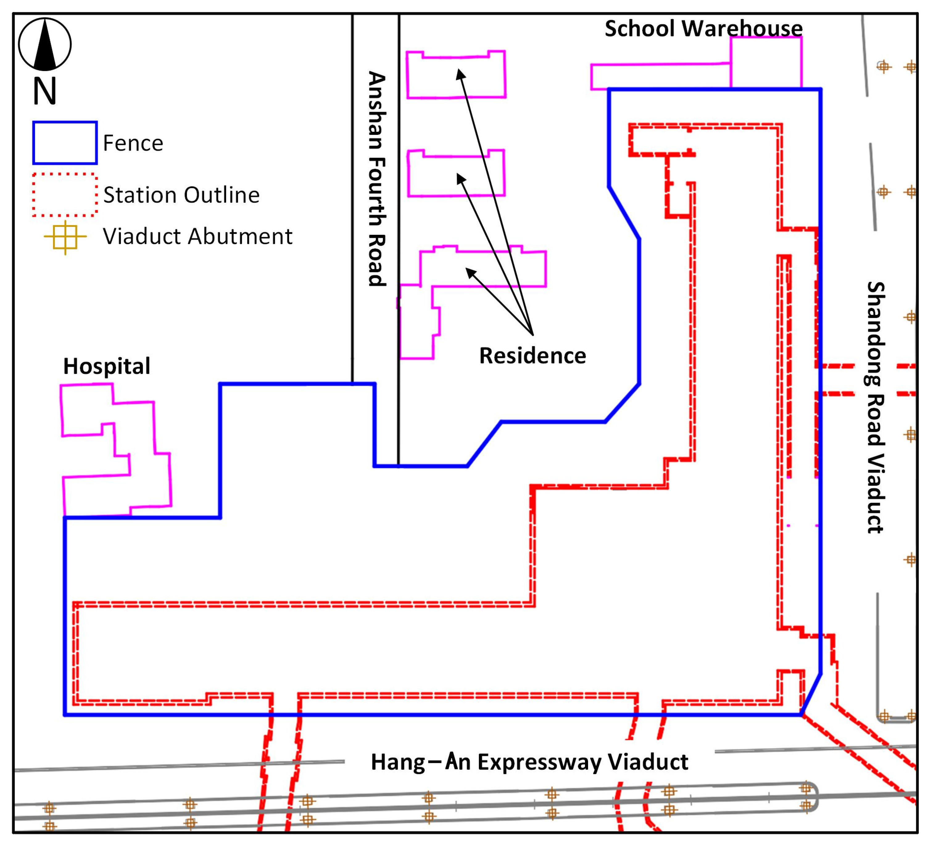
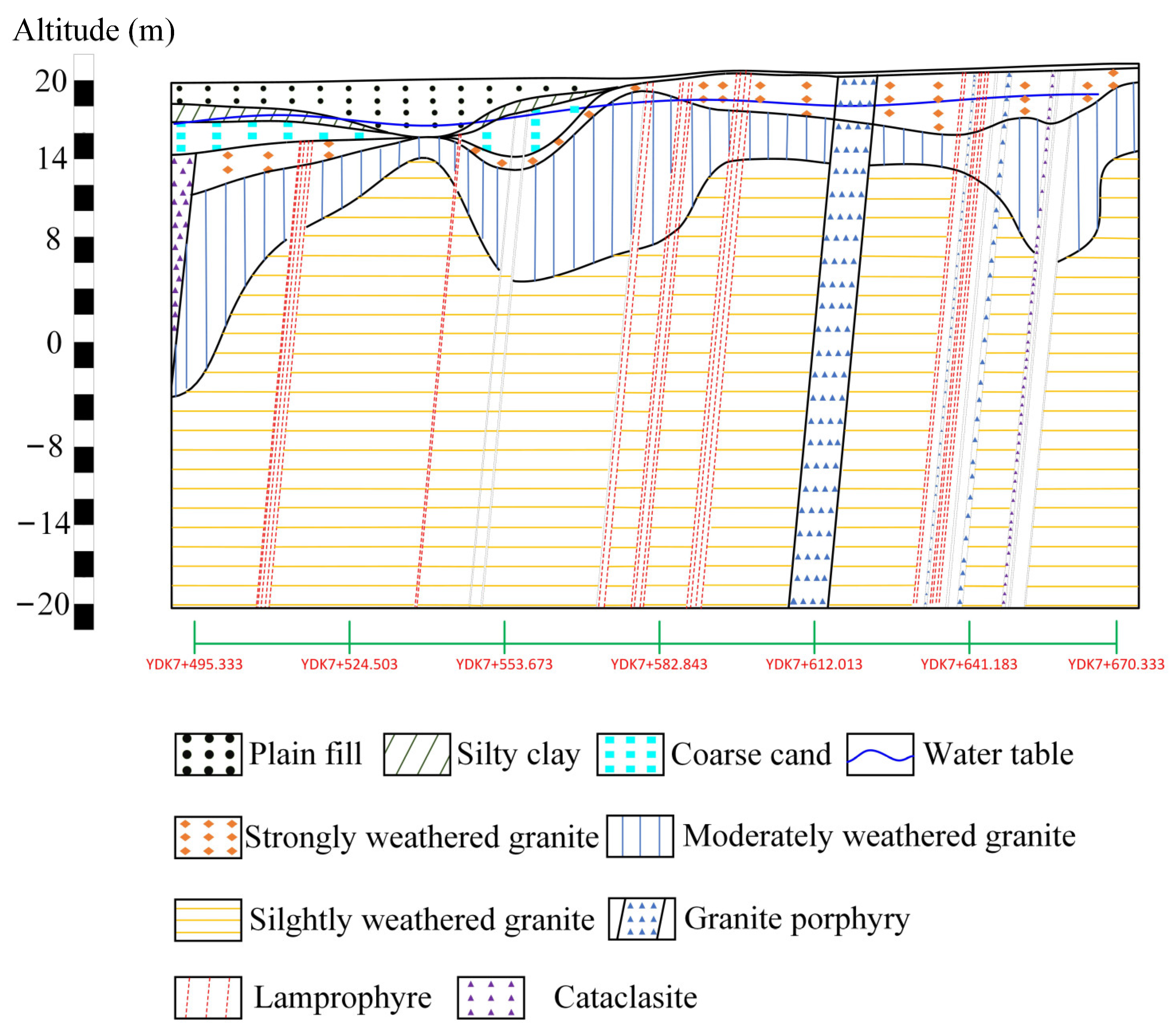
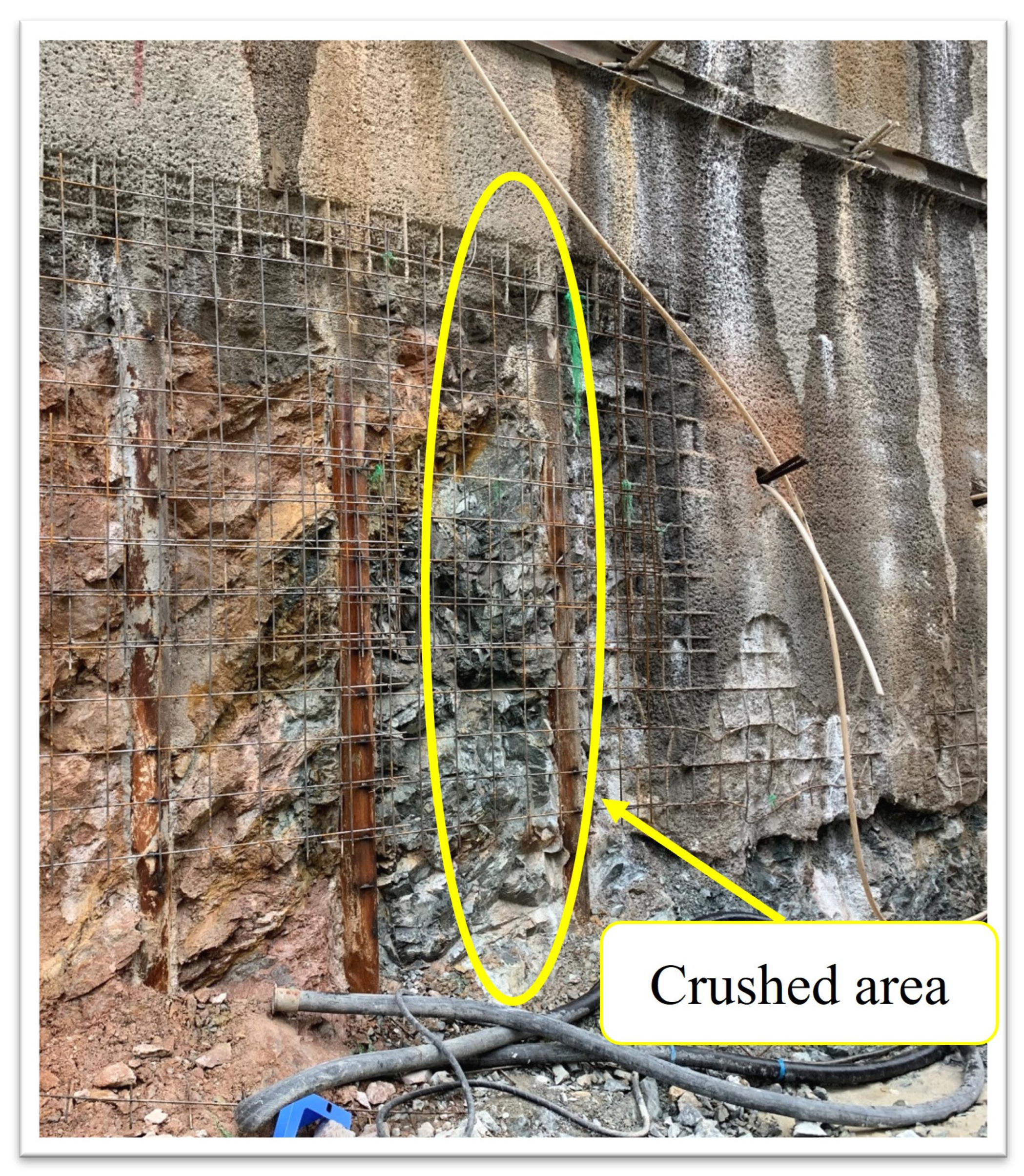
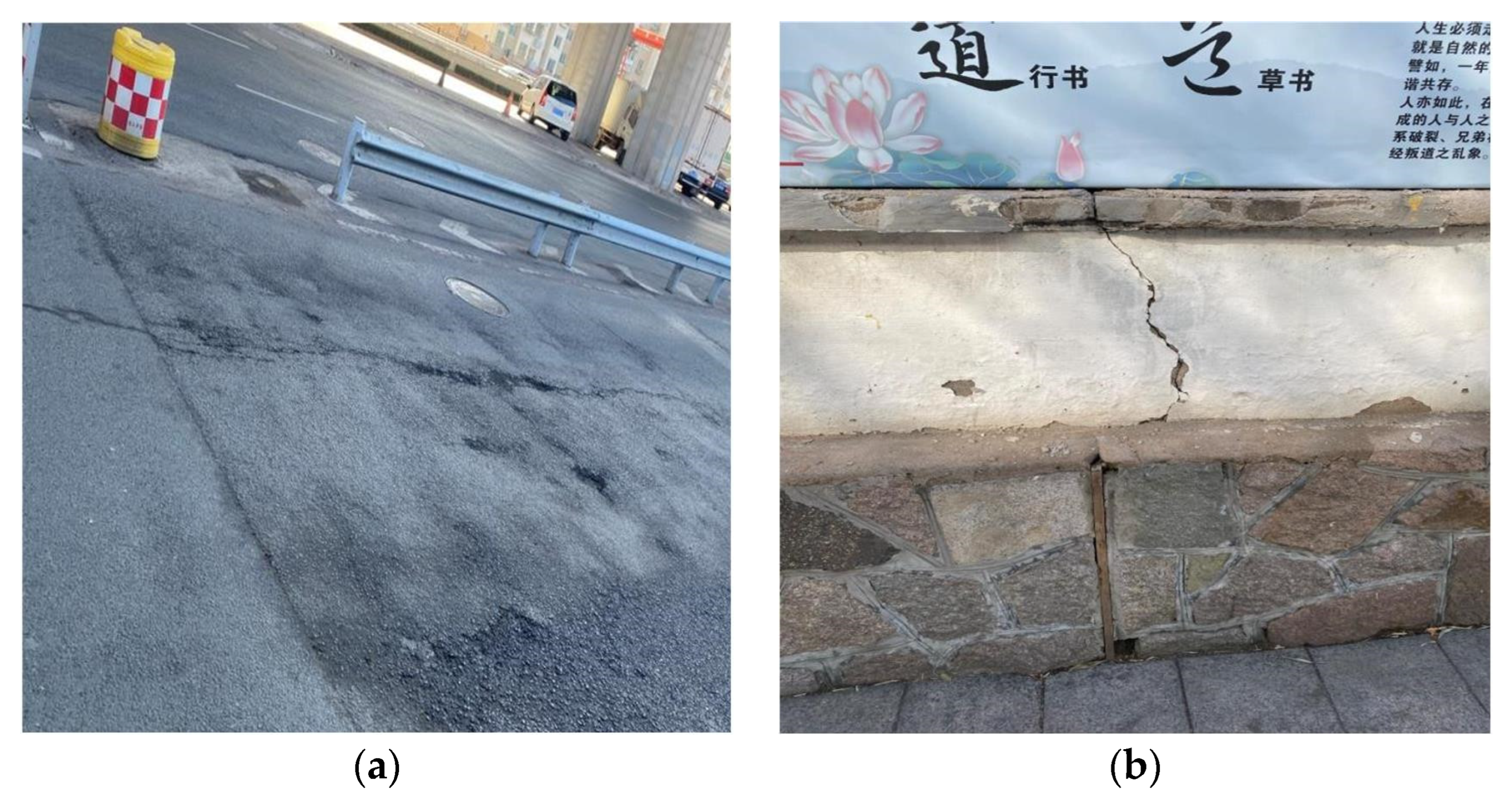
3.1. The Project
3.2. Excavation Risk Assessment
3.2.1. Evaluation Index System for Excavation Instability Risk
3.2.2. Risk Assessment Process Based on Improved Neural Networks
4. Conclusions
- The combined weights method is effective in screening potential risk factors. In this paper, a factor selection model was first constructed. The UR was used for the preliminary identification of potential risk factors. Then, the AHP-entropy method was applied to calculate the combined weights of the factors, with which the risk factors were selected. This factor selection model was valid, as verified through gray correlation analysis;
- An excavation risk evaluation index system was established for dynamic assessment. The dynamic evaluation of excavation safety was realized based on the improved RBF network, using real-time monitoring data as an evaluation index. A risk assessment of unit K was conducted and the risk grades at 10 January 2019 and 30 May 2019 were class II and class III, respectively. Additionally, comparison of the prediction results with different models verified the validity of the proposed model. The model in this paper had better accuracy and was less dependent on the original data.
- The model needs further improvement. The model could dynamically analyze the influence of each factor on the risk level of a deep excavation with soil–rock combination in construction. This has significant value in preventing excavation disasters and reducing unnecessary losses. However, a number of drawbacks remain, limiting further applications. This model needs to be gradually improved through continuous application.
Author Contributions
Funding
Institutional Review Board Statement
Informed Consent Statement
Data Availability Statement
Conflicts of Interest
References
- Lin, S.S.; Shen, S.L.; Zhou, A.; Xu, Y.S. Risk assessment and management of excavation system based on fuzzy set theory and machine learning methods. Autom. Constr. 2021, 122, 103490. [Google Scholar] [CrossRef]
- Liu, J.C.; Tan, Y. Review of through-wall leaking incidents during excavation of the subway stations of Nantong metro line 1 in thick water-rich sandy strata. Tunn. Undergr. Space Technol. 2023, 135, 105056. [Google Scholar] [CrossRef]
- Huang, L.W.; Xu, Y.L.; Zhou, K.; Wang, G.W. Analysis on the collapse causes of foundation pit under complex environmental in soft soil areas. Chin. J. Undergr. Space Eng. 2023. [Google Scholar]
- Wang, K.; Gao, Y.; Jin, Z.; Zhou, X.; Chen, L.; Zhang, C. Research on stability of steep bank slope and reserved thin-walled rock cofferdam during excavation of intake foundation pit. Eng. Fail. Anal. 2022, 141, 106659. [Google Scholar] [CrossRef]
- Oztoprak, S.; Cinicioglu, S.F.; Oztorun, N.K.; Alhan, C. Impact of neighbouring deep excavation on high-rise sun plaza building and its surrounding. Eng. Fail. Anal. 2020, 111, 104495. [Google Scholar] [CrossRef]
- Sousa, R.L.; Einstein, H.H. Lessons from accidents during tunnel construction. Tunn. Undergr. Space Technol. 2021, 113, 103916. [Google Scholar] [CrossRef]
- Zhao, Y.; Chen, X.; Hu, B.; Huang, L.; Lu, G.; Yao, H. Automatic monitoring and control of excavation disturbance of an ultra-deep foundation pit extremely adjacent to metro tunnels. Tunn. Undergr. Space Technol. 2023, 142, 105445. [Google Scholar] [CrossRef]
- Li, Y.; Zhou, G.; Li, T.; Tang, C.; Gong, B.; Wang, K. Influence of tunnel excavation on the deformation of a frame building. Buildings 2023, 13, 810. [Google Scholar] [CrossRef]
- Liang, Z.; Gong, B.; Wu, X.; Zhang, Y.; Tang, C. Influence of principal stresses on failure behavior of underground openings. Chin. J. Rock Mech. Eng. 2015, 34, 3176–3187. [Google Scholar]
- Liang, Z.; Gong, B.; Li, W. Instability analysis of a deep tunnel under triaxial loads using a three-dimensional numerical method with strength reduction method. Tunn. Undergr. Space Technol. 2019, 86, 51–62. [Google Scholar] [CrossRef]
- Chen, B.; Gong, B.; Wang, S.; Tang, C. Research on zonal disintegration characteristics and failure mechanisms of deep tunnel in jointed rock mass with strength reduction method. Mathematics 2022, 10, 922. [Google Scholar] [CrossRef]
- Zhang, Y.; Zhang, W.; Xia, H.; Gong, B.; Liu, F.; Zhang, J.; Liu, K. Case Study and Risk Assessment of Water Inrush Disaster in Qingdao Metro Line 4. Appl. Sci. 2023, 13, 3384. [Google Scholar] [CrossRef]
- Finno, R.J.; Bryson, S.; Calvello, M. Performance of a stiff support system in soft clay. J. Geotech. Geoenviron. Eng. 2002, 128, 660–671. [Google Scholar] [CrossRef]
- Son, M.; Cording, E.J. Estimation of building damage due to excavation-induced ground movements. J. Geotech. Geoenviron. Eng. 2005, 131, 162–177. [Google Scholar] [CrossRef]
- Shen, S.L.; Lin, S.S.; Zhou, A. A cloud model-based approach for risk analysis of excavation system. Reliab. Eng. Syst. Saf. 2023, 231, 108984. [Google Scholar] [CrossRef]
- Zhang, X.; An, J. A new pre-assessment model for failure-probability-based-planning by neural network. J. Loss Prev. Process Ind. 2023, 81, 104908. [Google Scholar] [CrossRef]
- Zhao, J.; Ritter, S.; DeJong, M.J. Early-stage assessment of structural damage caused by braced excavations: Uncertainty quantification and a probabilistic analysis approach. Tunn. Undergr. Space Technol. 2022, 125, 104499. [Google Scholar] [CrossRef]
- Choi, H.H.; Cho, H.N.; Seo, J.W. Risk assessment methodology for underground construction projects. J. Constr. Eng. Manag. 2004, 130, 258–272. [Google Scholar] [CrossRef]
- Zhou, H.B.; Zhang, H. Risk assessment methodology for a deep foundation pit construction project in Shanghai, China. J. Constr. Eng. Manag. 2011, 137, 1185–1194. [Google Scholar] [CrossRef]
- Zhou, Y.; Li, S.; Zhou, C.; Luo, H. Intelligent approach based on random forest for safety risk prediction of deep foundation pit in subway stations. J. Comput. Civ. Eng. 2019, 33, 05018004. [Google Scholar] [CrossRef]
- Gong, B.; Tang, C.A.; Wang, S.Y.; Bai, H.M.; Li, Y.C. Simulation of the nonlinear mechanical behaviors of jointed rock masses based on the improved discontinuous deformation and displacement method. Int. J. Rock Mech. Min. Sci. 2019, 122, 104076. [Google Scholar] [CrossRef]
- Feng, X.H.; Gong, B.; Cheng, X.F.; Zhang, H.H.; Tang, C.A. Anisotropy and microcrack-induced failure precursor of shales under dynamic splitting. Geomat. Nat. Hazards Risk 2022, 13, 2864–2889. [Google Scholar] [CrossRef]
- Wang, Y.Y.; Gong, B.; Tang, C.A. Numerical investigation on anisotropy and shape effect of mechanical properties of columnar jointed basalts containing transverse joints. Rock Mech. Rock Eng. 2022, 55, 7191–7222. [Google Scholar] [CrossRef]
- Wang, Y.; Gong, B.; Zhang, Y.; Yang, X.; Tang, C. Progressive fracture behavior and acoustic emission release of CJBs affected by joint distance ratio. Mathematics 2022, 10, 4149. [Google Scholar] [CrossRef]
- Liang, Z.; Gong, B.; Tang, C.; Zhang, Y.; Ma, T. Displacement back analysis for a high slope of the Dagangshan Hydroelectric Power Station based on BP neural network and particle swarm optimization. Sci. World J. 2014, 2014, 741323. [Google Scholar] [CrossRef]
- Chen, X.S.; Hong, C.Y.; Su, D. Intelligent geotechnical engineering. Chin. J. Geotech. Eng. 2022, 44, 2151–2159. [Google Scholar]
- Hegde, J.; Rokseth, B. Applications of machine learning methods for engineering risk assessment-A review. Saf. Sci. 2020, 122, 104492. [Google Scholar] [CrossRef]
- Gong, B. Study of PLSR-BP model for stability assessment of loess slope based on particle swarm optimization. Sci. Rep. 2021, 11, 17888. [Google Scholar] [CrossRef]
- Zhang, C.; Li, J.Z.; He, Y. Application of optimized grey discrete Verhulst–BP neural network model in settlement prediction of foundation pit. Environ. Earth Sci. 2019, 78, 441. [Google Scholar] [CrossRef]
- Shen, Y.S.; Wang, P.; Li, M.P.; Mei, Q.W. Application of subway foundation pit engineering risk assessment: A case study of Qingdao rock area, China. KSCE J. Civ. Eng. 2019, 23, 4621–4630. [Google Scholar] [CrossRef]
- Lin, S.S.; Zhang, N.; Zhou, A.; Shen, S.L. Risk evaluation of excavation based on fuzzy decision-making model. Autom. Constr. 2022, 136, 104143. [Google Scholar] [CrossRef]
- Sou-Sen, L.; Hsien-Chuang, L. Neural-network-based regression model of ground surface settlement induced by deep excavation. Autom. Constr. 2004, 13, 279–289. [Google Scholar] [CrossRef]
- Li, X.; Pan, Y.; Zhang, L.; Chen, J. Dynamic and explainable deep learning-based risk prediction on adjacent building induced by deep excavation. Tunn. Undergr. Space Technol. 2023, 140, 105243. [Google Scholar] [CrossRef]
- Lü, Q.; Chan, C.L.; Low, B.K. Probabilistic evaluation of ground-support interaction for deep rock excavation using artificial neural network and uniform design. Tunn. Undergr. Space Technol. 2012, 32, 1–18. [Google Scholar] [CrossRef]
- Kounlavong, K.; Keawsawasvong, S.; Wipulanusat, W.; Jamsawang, P. Physics-based and data-driven modeling for basal stability evaluation of braced excavations in natural clays. Heliyon 2023, 9, 10. [Google Scholar]
- Ning, X.; An, Y.; Ju, L.; Wang, W. Real-time online prediction of surface settlement considering spatiotemporal characteristics during foundation excavation. Autom. Constr. 2023, 150, 104831. [Google Scholar] [CrossRef]
- Tang, Y.; Xiao, S.; Zhan, Y. Predicting settlement along railway due to excavation using empirical method and neural networks. Soils Found. 2019, 59, 1037–1051. [Google Scholar] [CrossRef]
- Tao, Y.; Sun, H.; Cai, Y. Predictions of deep excavation responses considering model uncertainty: Integrating BiLSTM neural networks with Bayesian updating. Int. J. Geomech. 2022, 22, 04021250. [Google Scholar] [CrossRef]
- Liu, Y.; Yang, Z.; Li, X. Adaptive ensemble learning of radial basis functions for efficient geotechnical reliability analysis. Comput. Geotech. 2022, 146, 104753. [Google Scholar] [CrossRef]
- Huang, Z.K.; Zhang, D.M.; Xie, X.C. A practical ANN model for predicting the excavation-induced tunnel horizontal displacement in soft soils. Undergr. Space 2022, 7, 278–293. [Google Scholar] [CrossRef]
- Chen, R.P.; Zhang, P.; Kang, X.; Zhong, Z.Q.; Liu, Y.; Wu, H.N. Prediction of maximum surface settlement caused by earth pressure balance (EPB) shield tunneling with ANN methods. Soils Found. 2019, 59, 284–295. [Google Scholar] [CrossRef]
- Liu, B.; Wang, R.; Zhao, G.; Guo, X.; Wang, Y.; Li, J.; Wang, S. Prediction of rock mass parameters in the TBM tunnel based on BP neural network integrated simulated annealing algorithm. Tunn. Undergr. Space Technol. 2020, 95, 103103. [Google Scholar] [CrossRef]
- Zhang, R.; Tian, D.; Wang, H.; Kang, X.; Wang, G.; Xu, L. Risk Assessment of Compound Dynamic Disaster Based on AHP-EWM. Appl. Sci. 2023, 13, 10137. [Google Scholar] [CrossRef]
- Chen, J.; Liu, Y. Locally linear embedding: A survey. Artif. Intell. Rev. 2011, 36, 29–48. [Google Scholar] [CrossRef]
- Kavvadas, M.J. Monitoring ground deformation in tunnelling: Current practice in transportation tunnels. Eng. Geol. 2005, 79, 93–113. [Google Scholar] [CrossRef]
- Masini, L.; Gaudio, D.; Rampello, S.; Romani, E. Observed performance of a deep excavation in the historical center of Rome. J. Geotech. Geoenviron. Eng. 2021, 147, 05020015. [Google Scholar] [CrossRef]
- GB 50497-2009; Technical Standard for Monitoring of Building Excavation Engineering. Ministry of Housing and Urban-Rural Development of the People’s Republic of China, Planning Publishing House: Beijing, China, 2009.
- GB 50911-2013; Code for Monitoring Measurement of Urban Rail Transit Engineering. Ministry of Housing and Urban-Rural Development of the People’s Republic of China, China Architecture & Building Press: Beijing, China, 2014.


| Definition | Definition | ||
|---|---|---|---|
| 1 | Equal importance | 2 | Between weak and equal importance |
| 3 | Weak importance | 4 | Between essential or strong and weak importance |
| 5 | Essential or strong importance | 6 | Between demonstrated and essential or strong |
| 7 | Demonstrated importance | 8 | |
| 9 | Absolute importance |
| Matrix Order | 1 | 2 | 3 | 4 | 5 |
|---|---|---|---|---|---|
| RI | 0 | 0 | 0.52 | 0.89 | 1.12 |
| Guideline Layer | Potential Risk Factors | UR | Judgements |
|---|---|---|---|
| The environment in the excavation | Soil stress C11 | 0.9 | Fit |
| Microseismic grade C12 | 0.81 | Fit | |
| Weak rock thickness C13 | 0.67 | Fit | |
| Microseismic frequency C14 | 0.67 | Fit | |
| Special strata C15 | 0.3 | Unfit | |
| The environment around the excavation | Thickness of overburden C21 | 0.9 | Fit |
| Deformation of neighboring buildings C22 | 0.81 | Fit | |
| Surface settlement C23 | 0.7 | Fit | |
| Water table C24 | 0.67 | Fit | |
| The excavation support structure | Vertical deformation C31 | 0.81 | Fit |
| Transverse deformation C32 | 0.81 | Fit | |
| Anchor cable axial force C33 | 0.83 | Fit |
| Expert 1 | Expert 2 | Expert 3 | Average Weight | CR | Entropy Value | Entropy Weight | Comprehensive Weight | |
|---|---|---|---|---|---|---|---|---|
| C11 | 0.23 | 0.17 | 0.23 | 0.21 | <0.1 | 0.934 | 0.036 | 0.199 |
| C12 | 0.14 | 0.17 | 0.14 | 0.15 | 0.811 | 0.104 | 0.141 | |
| C13 | 0.49 | 0.33 | 0.49 | 0.44 | 0.934 | 0.036 | 0.435 | |
| C14 | 0.14 | 0.33 | 0.14 | 0.2 | 0.680 | 0.177 | 0.193 | |
| C21 | 0.09 | 0.11 | 0.11 | 0.1 | <0.1 | 0.931 | 0.038 | 0.086 |
| C22 | 0.66 | 0.54 | 0.45 | 0.55 | 0.979 | 0.012 | 0.548 | |
| C23 | 0.17 | 0.18 | 0.34 | 0.23 | 0.727 | 0.151 | 0.208 | |
| C24 | 0.08 | 0.18 | 0.10 | 0.12 | 0.583 | 0.231 | 0.166 | |
| C31 | 0.27 | 0.31 | 0.43 | 0.34 | <0.1 | 0.922 | 0.043 | 0.317 |
| C32 | 0.27 | 0.58 | 0.43 | 0.43 | 0.879 | 0.067 | 0.386 | |
| C33 | 0.46 | 0.11 | 0.14 | 0.23 | 0.811 | 0.104 | 0.206 |
| Evaluation Index | Ⅰ | Ⅱ | Ⅲ | Ⅳ | |
|---|---|---|---|---|---|
| Soil stress C11 | MPa | ≤6 | 6 | 15 | 24 |
| Microseismic grade C12 | grade | ≤3 | 4 | 5 | ≥6 |
| Weak rock thickness C13 | m | <6 | 6−12 | 12−18 | >18 |
| Microseismic frequency C14 | grade | weak | medium | comparatively strong | strong |
| Thickness of overburden C21 | mm | <2 | 2−5 | 5−8 | >8 |
| Deformation of neighboring buildings C22 | mm | <10 | 10−14 | 14−18 | >18 |
| Surface settlement C23 | mm | <12 | 12−18 | 18−24 | >24 |
| Water table C24 | mm | <500 | 500−1000 | 1000−1500 | >1500 |
| Vertical deformation C31 | mm | <18 | 18−24 | 24−30 | >30 |
| Transverse deformation C32 | mm | <12 | 12−17 | 17−25 | >25 |
| Anchor cable axial force C33 | MPa | <216 | 216−243 | 243−270 | >270 |
| Risk Level | Management Measures |
|---|---|
| Ⅰ | Continue construction and perform daily monitoring. |
| Ⅱ | Construction continues with more frequent monitoring and prohibit construction overruns. |
| Ⅲ | Construction is suspended with monitoring, while meetings are held to investigate the cause and prepare contingency measures. |
| Ⅳ | Stop construction and all personnel leave, while analyzing the cause, make an early warning and develop measures according to the emergency plan. |
| Parent Sequence | Correlation Coefficient | ||||||||||
|---|---|---|---|---|---|---|---|---|---|---|---|
| C11 | C12 | C13 | C14 | C21 | C22 | C23 | C24 | C31 | C32 | C33 | |
| Ⅰ | 0.9271 | 0.9119 | 0.9882 | 0.4541 | 0.8392 | 0.9359 | 0.7927 | 0.7798 | 0.9024 | 0.9690 | 0.7823 |
| Ⅱ | 0.7665 | 0.7747 | 0.9766 | 0.6940 | 1.0000 | 0.8589 | 0.6889 | 0.9084 | 0.8253 | 0.8067 | 0.6673 |
| Ⅲ | 0.9271 | 0.9330 | 0.8267 | 0.9455 | 0.7229 | 0.8203 | 0.7235 | 0.9520 | 0.8269 | 0.8281 | 0.7272 |
| Ⅳ | 0.9271 | 0.9551 | 0.8267 | 0.4541 | 1.0000 | 0.8203 | 0.9642 | 0.9520 | 0.9558 | 0.9690 | 0.8954 |
| Risk Level | Quantified Indexes | |||||||||||
|---|---|---|---|---|---|---|---|---|---|---|---|---|
| C11 | C12 | C13 | C14 | C21 | C22 | C23 | C24 | C31 | C32 | C33 | ||
| 1 | Ⅱ | 7.87 | 1.0 | 7.90 | 0.54 | 12.32 | −2.95 | −7.65 | −5869 | −11.04 | 12.29 | 275.83 |
| 2 | Ⅲ | 10.23 | 1.86 | 10.78 | 0.57 | 17.30 | −1.88 | −5.0 | −5711 | −8.74 | 15.09 | 294.06 |
| 3 | Ⅰ | 6.16 | 0.45 | 4.32 | 0.37 | 8.09 | −3.58 | −9.36 | −6015 | −12.36 | 9.60 | 264.22 |
| 4 | Ⅳ | 11.67 | 1.56 | 10.96 | 0.68 | 19.68 | −1.77 | −6.45 | −5569 | −9.85 | 9.8 | 257.35 |
| 5 | Ⅱ | 5.47 | 2 | 8.45 | 0.60 | 17.68 | −2.25 | −7.65 | −5671 | −10.31 | 9.84 | 260.43 |
| 6 | Ⅳ | 11.16 | 1.69 | 10.22 | 0.81 | 22.70 | −4.63 | −9.23 | −6423 | −11.71 | 14.49 | 273.3 |
| 7 | Ⅱ | 3.77 | 1.21 | 5.77 | 0.35 | 8.96 | −1.5 | −8.45 | −5848 | −11.29 | 12.26 | 269.91 |
| 8 | Ⅱ | 3.64 | 0.68 | 5.44 | 0.20 | 4.89 | −3.71 | −10.06 | −6377 | −12.21 | 14.91 | 274.59 |
| 9 | Ⅳ | 5.63 | 1.05 | 9.54 | 0.55 | 10.48 | −4.22 | −10.95 | −7196 | −12.26 | 15.64 | 301.45 |
| 10 | Ⅲ | 8.37 | 0.96 | 4.58 | 0.49 | 8.54 | −4.84 | −10.91 | −6981 | −13.09 | 15.32 | 287.46 |
| 11 | Ⅰ | 3.55 | 0.18 | 3.27 | 0.31 | 6.78 | −1.39 | −4.47 | −5067 | −8.38 | 8.49 | 254.61 |
| 12 | Ⅳ | 10.51 | 1.93 | 10.87 | 0.74 | 19.64 | −1.61 | −6.26 | −5169 | −9.44 | 14.03 | 295.47 |
| Risk Level | ||||||||||||
|---|---|---|---|---|---|---|---|---|---|---|---|---|
| Predicted results | 2 | 3 | 1 | 4 | 2 | 4 | 2 | 2 | 4 | 3 | 1 | 4 |
| Actual result | Ⅱ | Ⅲ | Ⅰ | Ⅳ | Ⅱ | Ⅳ | Ⅱ | Ⅱ | Ⅳ | Ⅲ | Ⅰ | Ⅳ |
| Date | Horizontal Displacement of Pile Top | Pile Settlement | Deep Horizontal Displacement | Anchor Cable Stress | Surface Settlement | Building Settlement | Water Table |
|---|---|---|---|---|---|---|---|
| 10 January 2019 | 9.80 mm | −9.85 mm | 17.84 mm | 257.35 kN | −6.45 mm | −1.77 mm | −5569 mm |
| 30 May 2019 | 15.38 mm | −13.45 mm | 18.72 mm | 304.71 kN | −11.56 mm | −5.43 mm | −7151.00 mm |
| Date | Fuzzy Synthetic Evaluation Model | LLE-RBF | RBF | BP | |
|---|---|---|---|---|---|
| 10 January 2019 | Ⅱ | Ⅱ | Ⅱ | Ⅱ | Ⅲ |
| 30 May 2019 | Ⅲ | Ⅲ | Ⅲ | Ⅱ | Ⅲ |
| mean square error | 0.045 | 0.251 | 0.779 |
Disclaimer/Publisher’s Note: The statements, opinions and data contained in all publications are solely those of the individual author(s) and contributor(s) and not of MDPI and/or the editor(s). MDPI and/or the editor(s) disclaim responsibility for any injury to people or property resulting from any ideas, methods, instructions or products referred to in the content. |
© 2023 by the authors. Licensee MDPI, Basel, Switzerland. This article is an open access article distributed under the terms and conditions of the Creative Commons Attribution (CC BY) license (https://creativecommons.org/licenses/by/4.0/).
Share and Cite
Zhang, L.; Zhang, W.; Wang, Z.; Liu, S.; Liu, K. Instability Risk Assessment for Deep Excavation of Soil–Rock Combinations Containing Groundwater. Appl. Sci. 2023, 13, 12887. https://doi.org/10.3390/app132312887
Zhang L, Zhang W, Wang Z, Liu S, Liu K. Instability Risk Assessment for Deep Excavation of Soil–Rock Combinations Containing Groundwater. Applied Sciences. 2023; 13(23):12887. https://doi.org/10.3390/app132312887
Chicago/Turabian StyleZhang, Liwei, Weiguo Zhang, Zaiquan Wang, Sijia Liu, and Kai Liu. 2023. "Instability Risk Assessment for Deep Excavation of Soil–Rock Combinations Containing Groundwater" Applied Sciences 13, no. 23: 12887. https://doi.org/10.3390/app132312887