Abstract
Rolling bearings are the core transmission components of large-scale equipment. Once a fault occurs, the consequences may be catastrophic, posing a serious threat to life and the safety of the property. Aimed at the problem of rolling bearing faults, this paper analyzes the characteristics of different fault signals and proposes a fault diagnosis method based on fuzzy signals. Based on the definition of an incomplete mapping of a new connotation, this paper proposes a fuzzy fault diagnosis method by fuzzy mapping, gives a fuzzy signal processing algorithm, and discusses two judgment principles. Further, it carries out a vibration signal analysis of the rolling bearing. According to the fault diagnosis method in this paper, the fault rolling bearing is diagnosed. The experimental results show that the proposed method can effectively diagnose rolling bearing faults closer to their natural attributes and solves the problem of traditional generator bearing fault diagnosis that requires complex models and poor diagnosis speed. Further, it can be seen that the average time consumption of this method is reduced and the fault recognition accuracy rate is increased. Compared with the existing related methods, this proposed diagnosis method is superior to that of several existing methods. It not only has higher precision, stronger anti-noise capacity, and faster diagnosis speed, but also has lower effective information loss.
1. Introduction
Rolling bearings play an important role in the operation of large-scale equipment. As the most common component of rotating machinery and equipment, rolling bearings play the role of transmission and support, and their working conditions have a significant impact on the operating conditions of the entire equipment. Rolling bearings are widely used in mechanical production and other fields. There is a lag in the maintenance of bearings after their failure. Once the production is shut down, it can cause a lot of time and cost waste to the enterprise. It is necessary to detect failings with bearings in advance and warn relevant personnel in time for factories and enterprises. However, rolling bearings are also one of the most easily damaged parts. The accidents caused by them are difficult to recover from. Not only does production need to stop for maintenance and to replace parts, but also the maintenance costs are relatively high. According to statistics, approximately 30% of vibration faults in rotating machinery are caused by rolling bearing faults [1]. It can be seen that if the fault of the rolling bearing can be found and eliminated in time, the fault rate of the equipment will be greatly reduced. Therefore, it is of realistic research significance to research the fault diagnosis of rolling bearings.
The fault diagnosis technology of rolling bearings has been researched and developed for a long time, and there are three development stages in summary.
The first stage of development is mainly manual fault detection and analysis of equipment. In the early stages of industrial development, there were no sophisticated fault diagnosis instruments and fault detection could only be performed by experienced professionals. Due to the interference of human factors, this method has a certain degree of subjectivity, and there are often situations such as judgment errors or ignoring certain faults [2]. As a result, the fault diagnosis rate and adaptability are relatively low, causing abnormal heating, stalling, and abnormal vibration of engineering equipment, resulting in huge economic and personnel losses.
The second stage of development, first of all, is the time-domain analysis method. Commonly used time-domain characteristic index types include mean value, probability distribution, impulse index, density function, root mean square frequency, peak value, and kurtosis. Many scholars have conducted a lot of research on extracting time-domain features. Wang et al. [3] proposed a new method for predicting the fault state of rolling bearings by monitoring the vibration frequency and amplitude of the bearing seat. The method takes the kurtosis of the calculated vibration signal as the fault feature, and the kurtosis of the undamaged rolling bearing remains unchanged. The degree of damage to the bearing can be evaluated by the distribution of the kurtosis parameter in the selected frequency range. Larizza et al. [4] proposed that the periodic vibration peak generated by the rolling bearing at a constant speed is used as the fault characteristic signal, and the detection of the health status of the rolling bearing by the signal peak can improve the accuracy of diagnosis. Bao et al. [5] took kurtosis and mean square root as feature vectors at the same time, which can improve the fault recognition rate of rolling bearings. The fault diagnosis method based on time-domain features has the advantages of a simple calculation and fast diagnosis. However, it is difficult to extract effective fault information when extracting nonlinear and non-stationary vibration signal features. The next step is a frequency domain analysis. Many scholars have found many effective methods in the in-depth research and discussion of the frequency domain analysis method, such as amplitude-frequency spectrum, full pedigree, empirical mode decomposition, variational mode decomposition, envelope analysis, wavelet transform, etc. [6]. Empirical mode decomposition (EMD) has a good processing effect on time-domain and frequency domain data. Since the EMD method has an excellent processing effect on non-stationary feature information, it is often used in time-frequency domain signal analysis [7]. Some scholars have made further improvements to the EMD method by adding white noise to the vibration sequence to overcome the shortcomings of modal aliasing. This method is called ensemble empirical mode decomposition [8]. Li et al. [9] converted the vibration signal into a fast entropy fault characteristic map, which highlights the periodic fault pulse characteristics and improves the model’s anti-noise ability and stability. However, this method has certain limitations, and it is not obvious to the random vibration pulse. In the power distribution system, it is difficult to extract single-line ground fault characteristics and a diagnosis of fault. To solve this problem, Gao et al. [10] used the auto-encoder and fuzzy C-means clustering method to realize fault location and used the fuzzy C-means clustering method without threshold to perform feature classification to realize the fault diagnosis of a resonance grounding power distribution system. To effectively extract the features of non-stationary signals in heavy noise, Babiker et al. [11] proposed an improved fault diagnosis framework for variational modal decomposition and signal reporting, using the peak value and the maximum value of the correlation coefficient to calculate the best intrinsic mode function (IMF). Then, the IMF is reconstructed into a noise-reduction signal, and the early fault characteristics are accurately extracted. Li et al. [12] proposed a network framework for fault diagnosis based on local weighted multi-conditions and multi-labels, which uses the information contained in the encoder to realize fault diagnosis. Zhang et al. [13] proposed a multi-condition bearing fault pattern recognition framework, which uses compound multi-scale fuzzy entropy to efficiently extract fault feature information, and added a whale optimization algorithm to improve the training speed of support vector machine models and improve the fault pattern recognition rate.
In the third stage of development, with the iterative update of computer hardware, its ability to deal with complex problems has become stronger. Deep learning frameworks such as long- and short-term memory (LSTM) networks, fuzzy inference, support vector machines, decision trees, and convolutional neural networks have been implemented [14]. With the rapid development of machine learning algorithms and information system technology, intelligent diagnosis methods have also begun to be widely used in the field of rolling bearings. Intelligent diagnosis is based on different deep learning algorithms to preprocess vibration signals and extract deep features to achieve fault diagnosis [15]. Tian et al. [16] extracted the features through the variational modal decomposition of the original time series of the rolling bearing and then used the generalized regression network model to learn the feature information, train the model parameters, and use the maximum value normalization to achieve fault classification. The size of the traditional convolutional neural network convolution kernel is very small, and it ignores the detection and extraction of the overall information of the fault information feature distribution. Wang et al. [17] designed a one-dimensional visual convolutional neural network which uses a multi-layer small convolution kernel and a single-layer large convolution kernel to form a convolutional layer side by side. While the model improves the stability of the training process, it also improves the accuracy of the model’s recognition of rolling bearing faults. Since the automatic encoder has a good performance in feature extraction and size reduction, it is often used for fault diagnosis of rotating machinery [18]. Pu et al. [19] proposed restricted sparse networks based on the quadratic complex domain equation. Jiang et al. [20] proposed a rolling bearing fault diagnosis method based on variational mode decomposition and a grey wolf algorithm optimized extreme learning machine. These interpretation methods of rolling bearing fault features improved the detection speed but did not effectively improve the accuracy. Jandaghi et al. [21] introduced a new machine learning approach, called deterministic learning, for training soft robot models using radial basis function neural networks, based on which methods for machine fault detection are proposed. Using real engineering cases as the carrier, Yang and Jafarlou et al. [22,23,24] proposed the method of optimizing the signal analysis model and proposed the idea of fault detection. Darabi et al. [25] demonstrated, through extensive simulations, the effectiveness of STARNet in detecting untrusted sensor flows in both unimodal and multimodal environments, which is used to judge some fault signals. However, due to the severe lack of label data sets, it is difficult for existing autoencoders to extract a large number of effective fault features.
This article provides a new idea for traditional and complex fault diagnosis methods of rolling bearings, returning to the natural attributes of faults to realize fault diagnosis. This paper defines fuzzy mapping with new connotation features. Based on the original control advantages, combined with the fuzzy inference system, there is no need to establish a complex mathematical model for the rolling bearing; based on the constructed fuzzy mapping, a new difference algorithm and product algorithm are proposed, which are simple in operation and do not need to conduct data training. According to the calculation results of the former, a maximum method for individual fault diagnosis is proposed according to the “maximum approximation principle”, and an indirect method for group fault diagnosis is proposed according to the “minimum difference approximation principle”. The algorithm proposed is based on the defined set operation principle as a scientific theoretical basis. It provides a new way of thinking for fuzzy information control theory to deal with the actual fault problem with fuzzy signal, which can realize the fault diagnosis of rolling bearings more quickly and effectively.
2. Fuzzy Signal Analysis on Fault Diagnosis System
Aimed at analyzing the fault diagnosis method of rolling bearings, this paper constructs a diagnosis system based on fuzzy fault signals. A fuzzy signal refers to replacing a certain value of traditional fault data with an interval. The lower bound of the interval can be determined, while the upper bound is an uncertain value. The system consists of three parts:
(1) Analysis and processing of rolling bearing fault signals.
(2) Define the fault diagnosis function and give the fault diagnosis method.
(3) Conduct training and test experiments, as well as system stability training.
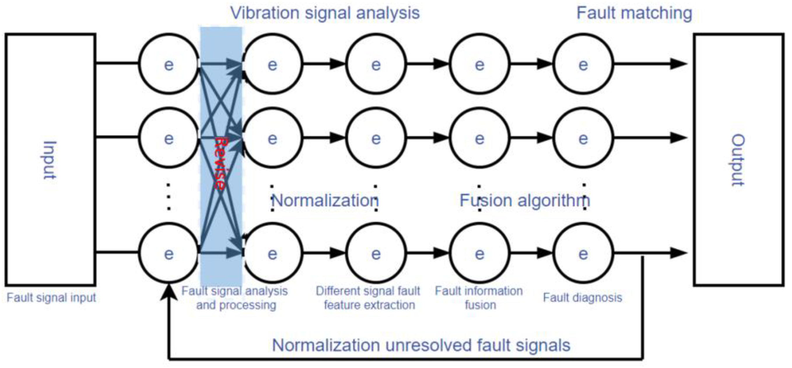
After the system has stabilized in training, it will be applied in practice. The specific working flow chart of the fuzzy signal fault diagnosis system is shown in Figure 1.
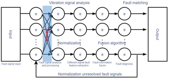
Figure 1.
Flow chart of fuzzy signal fault diagnosis system.
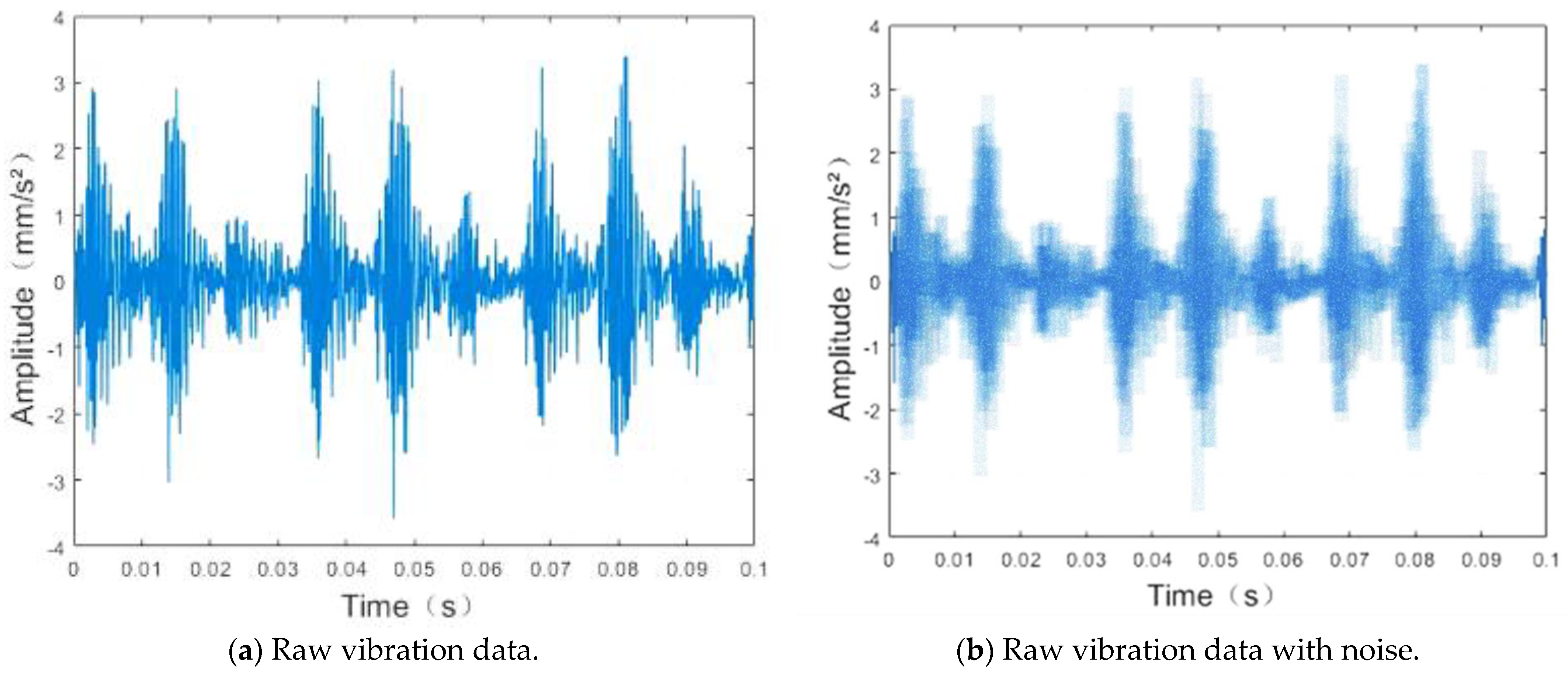
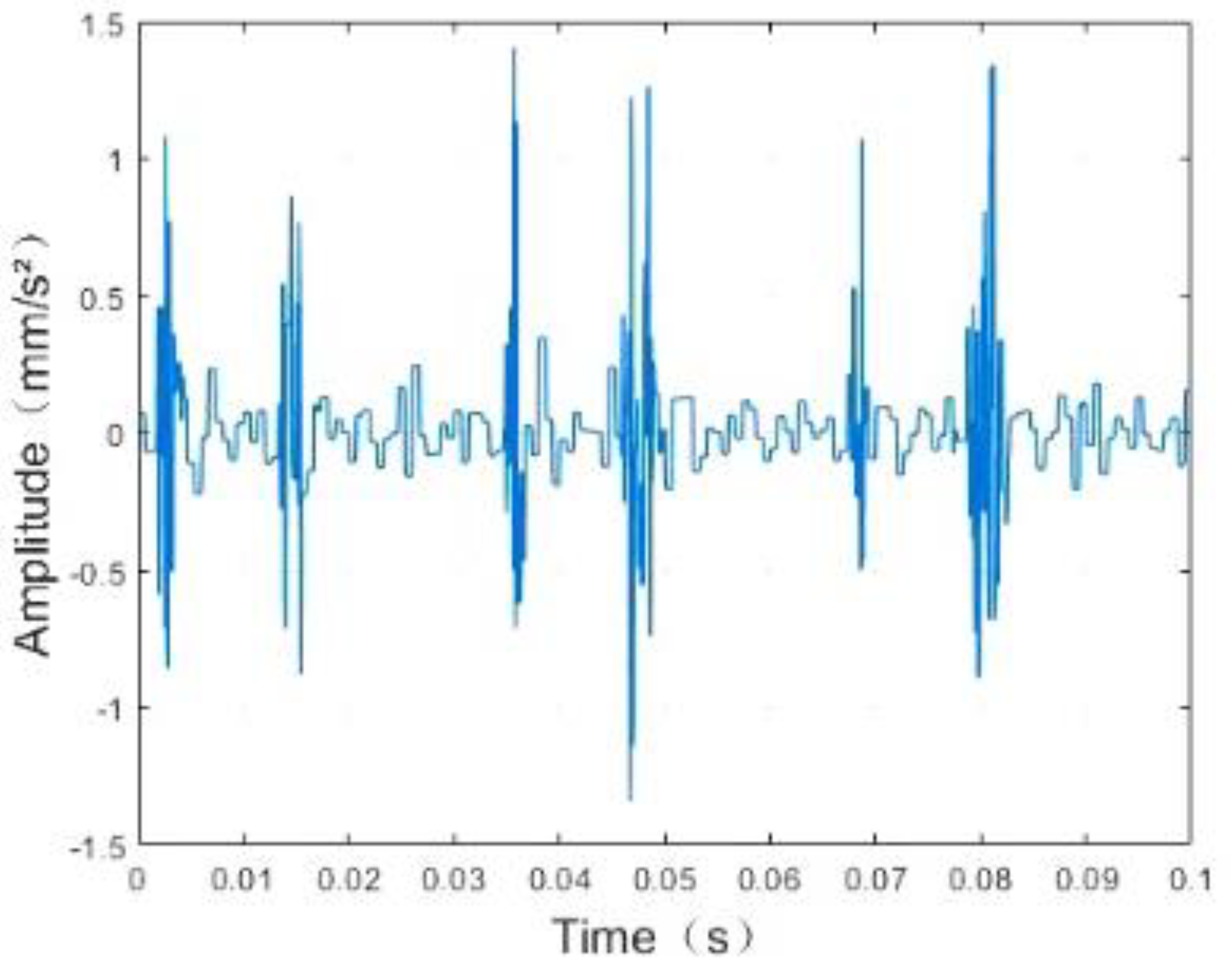
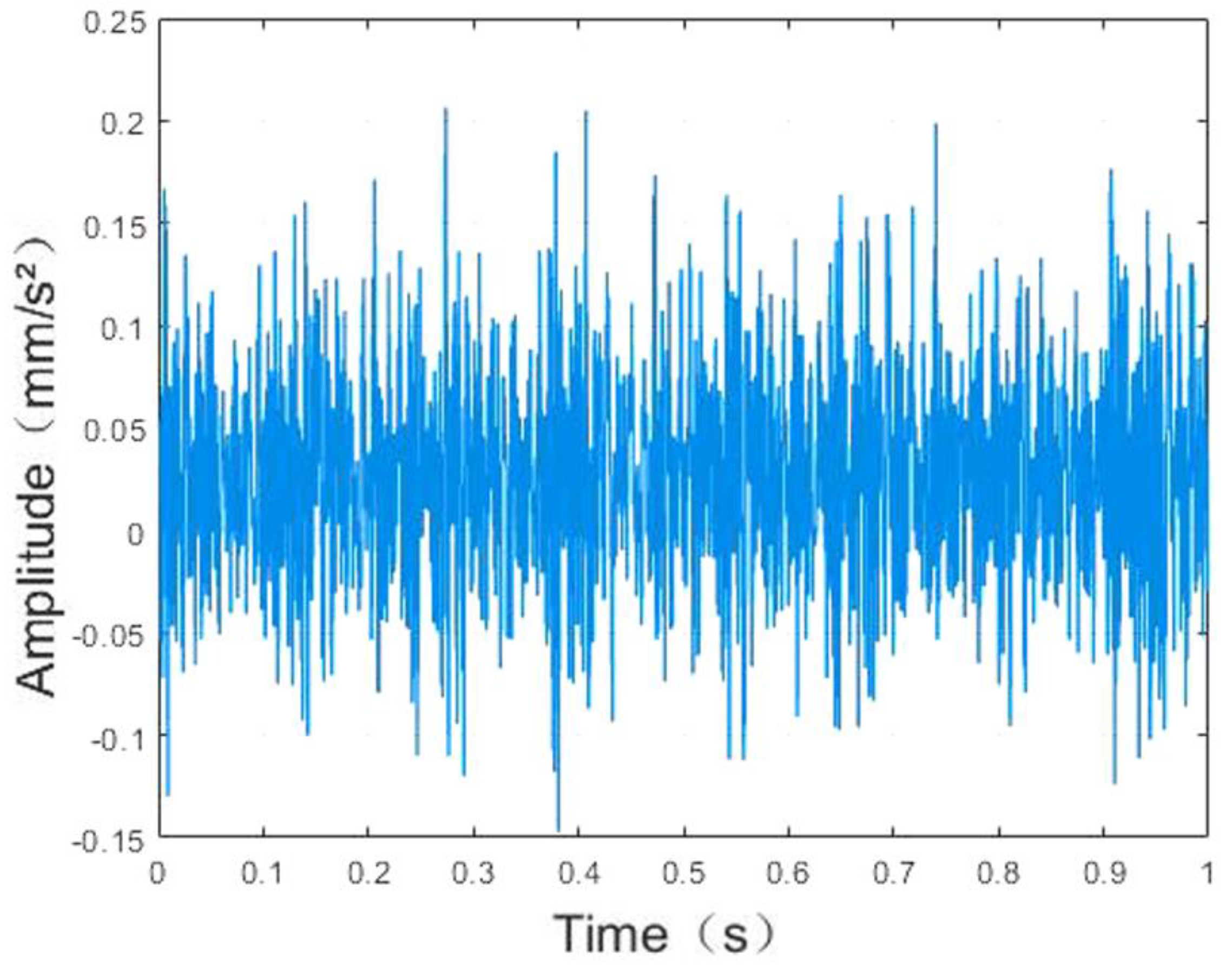
The vibration analysis method is widely used in the field of mechanical equipment fault diagnosis due to the advantages of easy acquisition of vibration signals and strong practicability. The vibration analysis method is currently the most used, and it is also one of the most sensitive and effective methods for the early diagnosis of small faults and has become the method for equipment fault diagnosis [26]. Therefore, this paper uses vibration signals to diagnose faults in rolling bearings. The discrete vibration signal collected in practice contains noise interference, and the original vibration signal data without denoising is shown in Figure 2a. Figure 2b illustrates the image after adding noise to the original signal. The waveform contains a large amount of useless low-amplitude noise data, which cannot highlight the high-amplitude features of the fault. Analyzing its amplitude characteristics, it can be seen that the shock pulse of the vibration signal at the time of fault increases rapidly at first and then slowly decays the oscillation in the form of an exponential. The signal is denoised and normalized. This system can reduce noise and optimize the amplitude of the fault characteristics based on the above-mentioned vibration signal fault characteristic analysis. The result is shown in Figure 3.
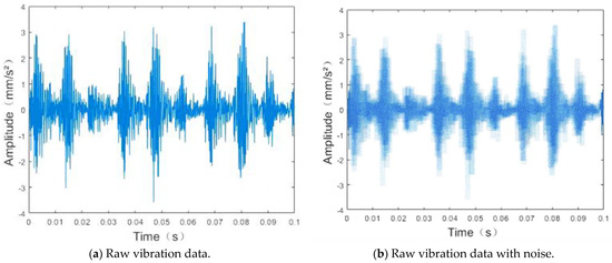
Figure 2.
Actually collected raw vibration data.
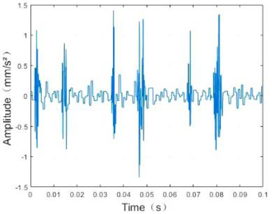
Figure 3.
The optimized vibration data of the system.
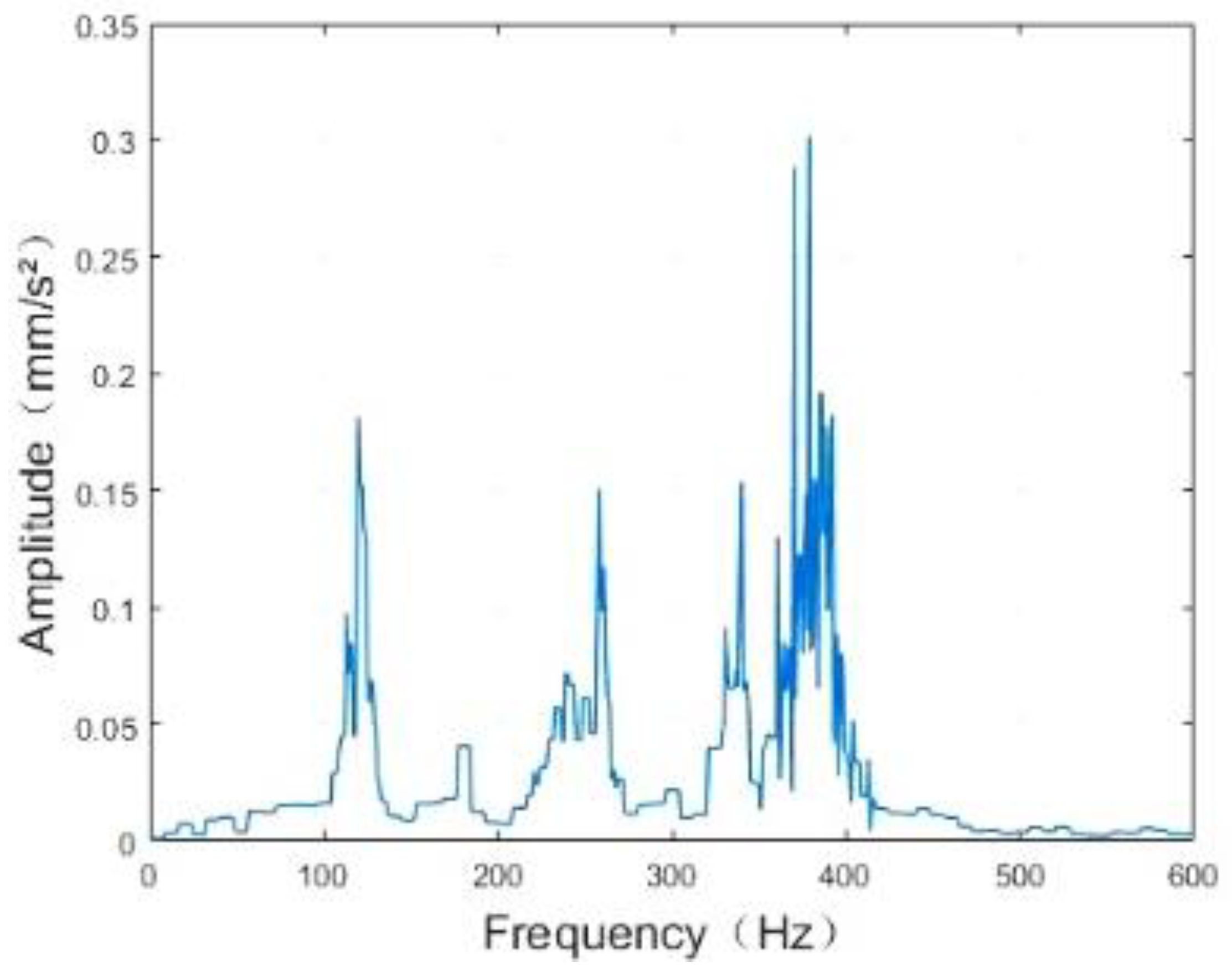
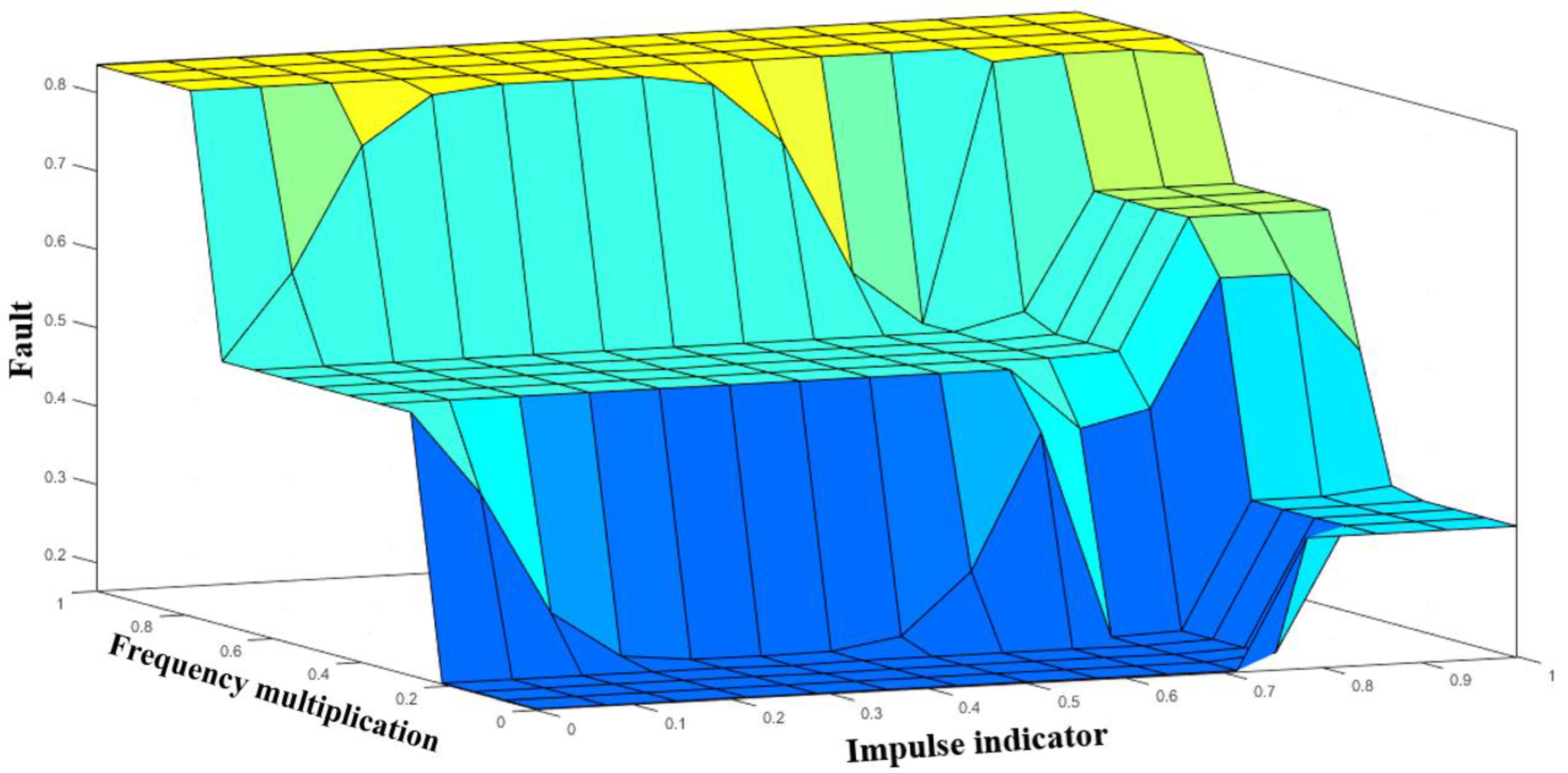
A single signal processing technology has made it difficult to meet the increasingly complex equipment fault diagnosis requirements [27]. Therefore, the optimized vibration data can be used for time-frequency analysis using this system, and the frequency domain characteristic signal of the fault data can be extracted by using frequency spectrum analysis, as shown in Figure 4. The system can fuse different fault signal characteristics for fault diagnosis and can customize fault classification according to the different needs of different objects. The visualized diagnosis result of the fusion of the two kinds of signal is shown in Figure 5.

Figure 4.
Time-frequency conversion result of this system.
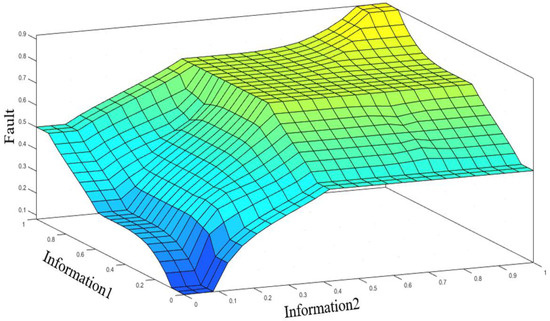
Figure 5.
Visualized results of fault diagnosis of the system.
After the system is completed, if the system stability requirements cannot be met, the system needs to be calibrated according to Formula (1).
where is the stability amplitude of the current system, and is the stability amplitude of the system at the previous moment. When the system is stable, usually needs to be less than the range of . The actual application can only be carried out when the stability of the system meets the requirements.
3. Fuzzy Fault Diagnosis Method
3.1. Fuzzy Mapping
Define the fuzzy signal set composed of two fuzzy signal sets . Suppose , the fuzzy signal set on the approximate space . and are the lower and upper approximations of , respectively. Proximity combination on , , there are three mappings on :
, there are , , and . Then, is the fuzzy signal set on . It can also be said that is a fuzzy signal set on . The totality of all sets B on A is BB as shown in Formula (3).
3.2. Fuzzy Signal Processing Algorithm
Define the fuzzy closeness vector function on . Suppose , , if the mapping satisfies the conditions:
(1) , and ;
(2) , , If , then ;
(3) If , then , and .
Then, is the fuzzy closeness vector function of the fuzzy signal sets and ; is the fuzzy closeness vector function on .
According to the definition of the fuzzy closeness vector function and the actual needs of this article, two specific fuzzy signal mapping processing algorithms are given below.
Difference algorithm: Define the difference fuzzy closeness vector function . If , then the fuzzy closeness vector function of the difference between and is shown in Equation (4).
where and belong to Set . , . The above content can be launched:
The proof process of Formula (4) is as follows:
(1) ,
(2) , ,
(3) If , then and , therefore, and . So, .
If is a closed domain on the real number domain, then the vector function of the fuzzy closeness of the difference between and is shown in Formula (6).
Among them, is the measure of , such as length, width, volume. The proof process of Formula (6) is similar to that of Formula (4), so it will not be proved any more.
Product algorithm: Define the product fuzzy closeness vector function . Suppose finite domain , and belong to Set . Where and ; , . The inner product of and on the fuzzy signal set is shown in Formula (7).
When generalizing to the fuzzy signal set on any domain , suppose the fuzzy signal set of the approximate space . The fuzzy signal sets and on belong to . The inner product of and is shown in Formula (8).
The dual operation of the inner product is an outer product. Suppose the fuzzy signal set of the approximate space . The fuzzy signal sets and on belong to . The outer product of and is shown in Formula (9).
Define the “remainder” operation on the closed interval . For , define the remainder of as . So, there is Formula (10).
Formula (9) is proved as follows:
Similar can prove .
For , let , . Where and are, respectively, called the upper approximation and the lower approximation of the closeness degree of on the fuzzy signal set.
Suppose are the set on fuzzy signal set . Let , then the following Formula (12) is established.
Especially when , , then .
According to Formula (12) and the definition of the fuzzy closeness vector function. Suppose fuzzy signal set on fuzzy signal set , then the product fuzzy closeness vector function of is shown in Equation (13).
3.3. Judgment Principle for Fault Diagnosis
Based on the above fuzzy signal processing algorithm, two specific judgment principles on fault diagnosis are given as follows:
- (1)
- Maximum method
Combined with the principle that a certain type of fault has the greatest probability, that type of fault will occur. A fault diagnosis method is given, which is called the maximum fault identification method. Suppose , denoted as , , for . If there is , Equation (14) is established.
where, , it is considered that is relatively close to fault . That is to say, and are the same type of fault.
- (2)
- Minimum difference method
Combining the principle that the difference between a certain type of fault and the actual fault characteristics is the smallest, the type of fault occurs. A fault diagnosis method is given, which is called the minimum difference fault identification method. Suppose fuzzy signal set , fault set . If there is , Equation (15) is established.
where , it is considered that the difference between and is the smallest. That is to say, and are the same type of fault.
4. Vibration Signal Analysis of Rolling Bearing
The vibration monitoring method is suitable for bearings of various types and working conditions. The vibration analysis method is widely used in the field of mechanical equipment fault diagnosis due to the advantages of easy acquisition of vibration signals and strong practicability. It is currently the most used and one of the most sensitive and effective methods for early diagnosis of small faults. It has become the main way to diagnose rolling bearing faults. Vibration signal monitoring and processing are simple, intuitive, and reliable in diagnosis. It contains the fault signal of the equipment, but the fault cannot be seen directly from the vibration signal. A series of processing and analysis of the vibration signal is required to obtain the fault characteristics. The fuzzy signal fault diagnosis system can analyze and process vibration signals.
It can be seen from Figure 6 that the vibration amplitude of the rolling bearing always fluctuates within a certain range under normal working conditions. When it exceeds this range and the amplitude presents periodic changes, it can be considered that the rolling bearing has failed. Therefore, the average value of multiple sets of normal working condition data can be calculated according to Formula (16) as the upper limit of the normal amplitude range (excluding outliers).
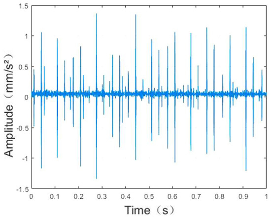
Figure 6.
The optimized vibration data of the system under normal working conditions.
Generally, the amplitude of the vibration signal exceeding the normal amplitude range is positively related to the impact force received by the bearing, so the impulse indicators in different periods can be used to reflect the degree of fault. The impulse index is shown in formula (17). Under normal circumstances, the fault amplitude is several times the normal amplitude, which is a number greater than 1. To better apply the algorithm proposed, the data should be normalized. The normalization formula is shown in Equation (18).
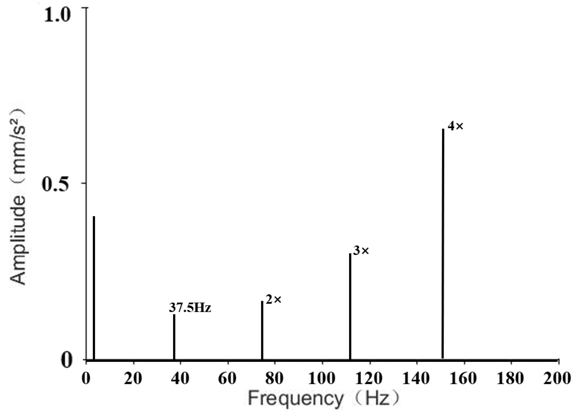
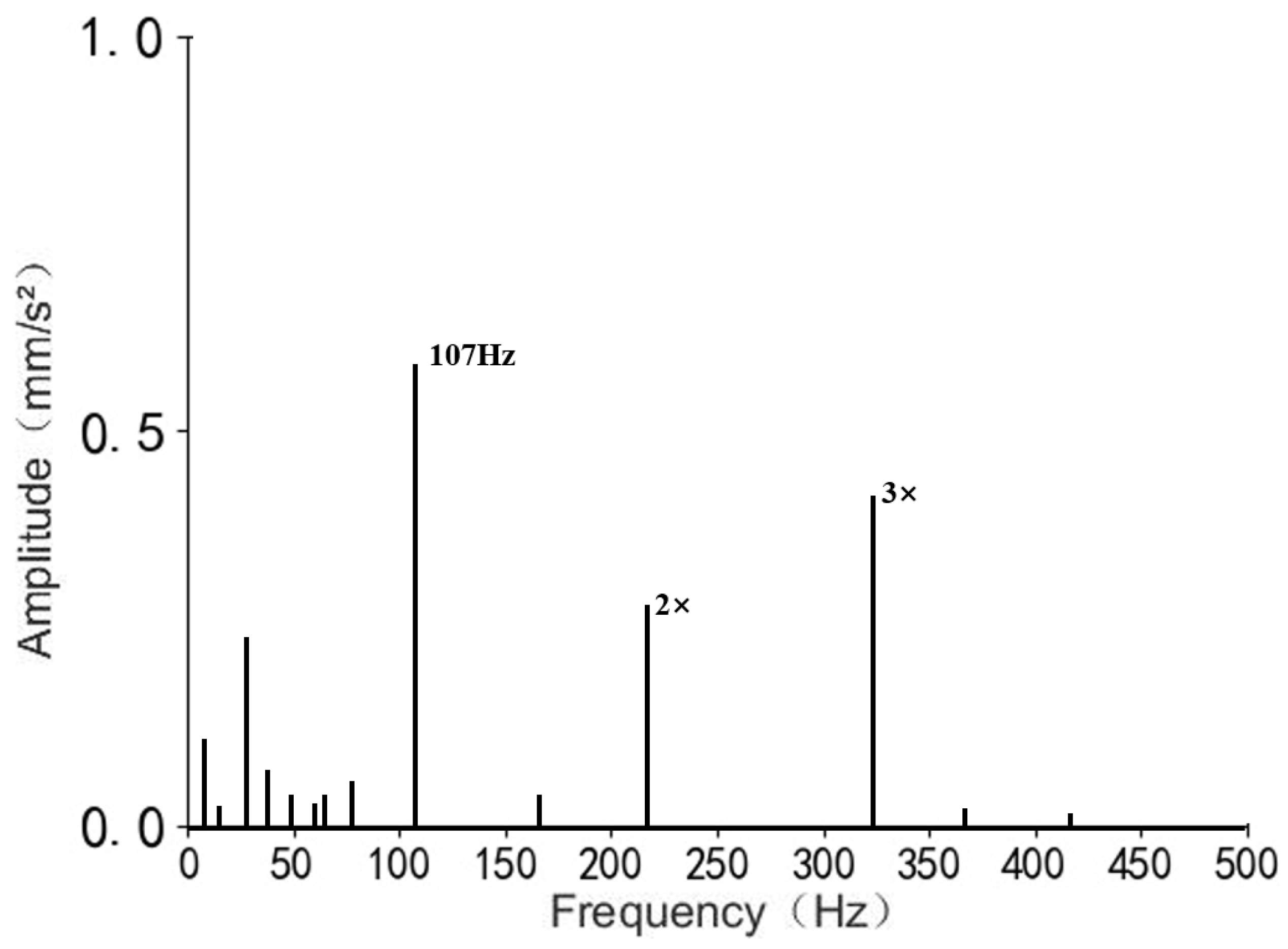
The degree of fault and the amplitude are only a positive correlation, not a strictly proportional relationship, so the degree of fault cannot be judged strictly. Therefore, relevant indicators of frequency can be integrated to accurately distinguish the degree of fault. Therefore, the physical quantity of “harmonic” can be fused to diagnose the degree of fault. Refer to the analysis of the power spectrum of the vibration signal of the paper machine dryer bearing fault, as shown in Figure 7. “2 times, 3 times, 4 times” harmonics appear in the picture. The more harmonics, the more serious the bearing fault. In addition, the fault frequency can be used to determine the outer race fault of the dryer bearing.
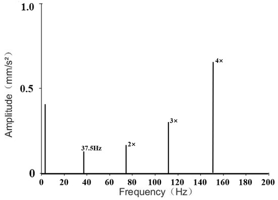
Figure 7.
Vibration power spectrum of dryer bearing.
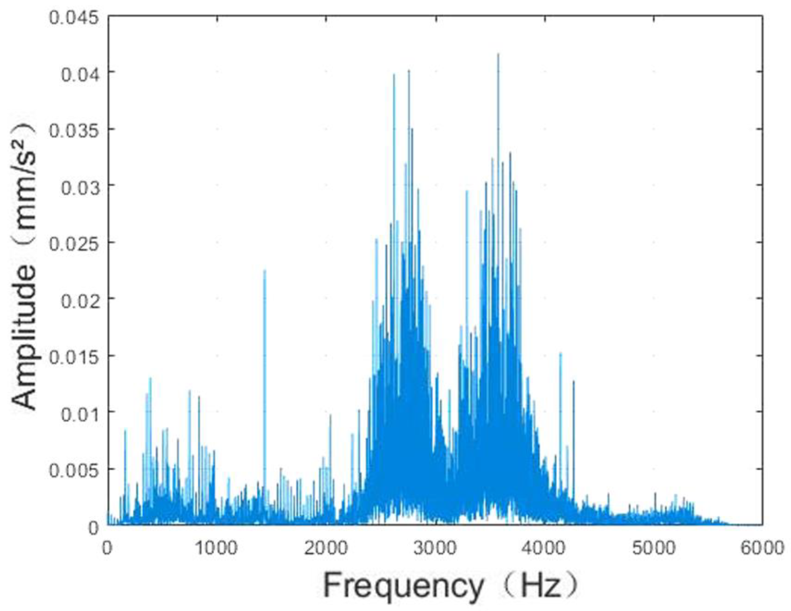
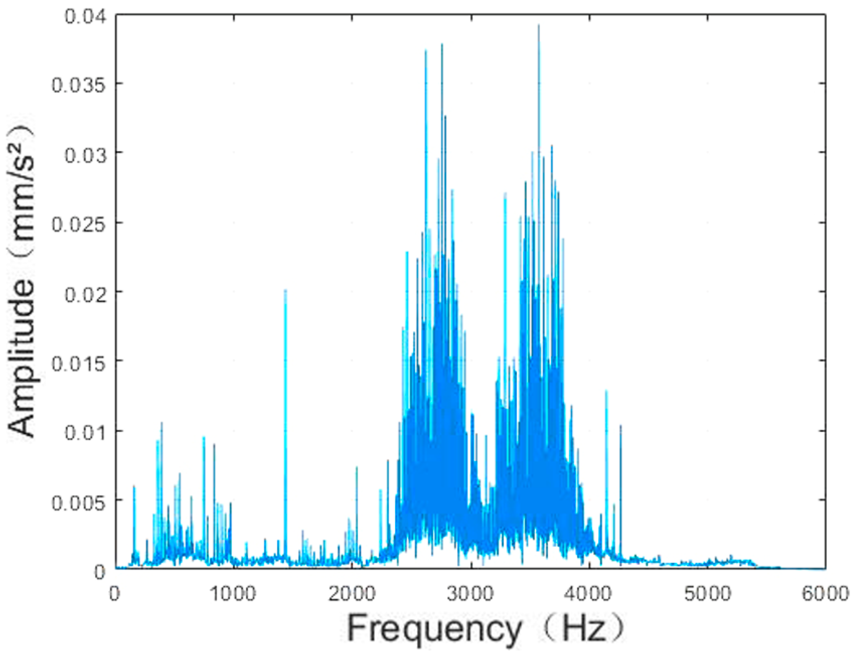
The fast Fourier transform (FFT) can convert the time-domain signal of the original discrete vibration data into a continuous frequency domain signal. It provides convenient conditions for fault diagnosis methods based on vibration signal spectrum analysis. For the same set of data shown in Figure 6, the FFT spectrogram is shown in Figure 8, and the analysis result of the time-frequency conversion of this system is shown in Figure 9. From the results, the time-frequency conversion of this system has a more obvious noise reduction effect than the FFT method, which provides a good data source for further obtaining harmonic signals from the power spectrum.

Figure 8.
The frequency spectrum of the fast Fourier transform.

Figure 9.
The frequency spectrum of time-frequency analysis of this system.
After obtaining the frequency spectrum, the fault location can be determined according to the rolling bearing fault frequency. When the bearing fails, it will produce regular vibration. Assuming that the rotation speed of the bearing is fixed, the time interval of the impact caused by the rotation inside the faulty bearing is also fixed; that is to say, the frequency of the impact is fixed. Therefore, this frequency is the fault frequency of the bearing. The fault frequency usually includes the fault frequency of the bearing outer race, ball, inner race, and cage. When the outer race does not rotate, the fault frequencies of the outer race raceway defects , the inner race raceway defects , and the ball defects are shown in Equation (19).
where is the pitch circle diameter, is the diameter of the ball, is the number of ball, is the contact angle of the ball, and is the relative rotation frequency of the inner and outer race of the bearing. Except for , the other parameters are the design parameters of the bearing. When the bearing model is determined, its calculated value is a constant and denoted as . Therefore, as long as is calculated, the fault frequency of the bearing at any speed can be known, and it can be determined where the bearing has failed.
5. Comparison of the Proposed Method with the Existing Method
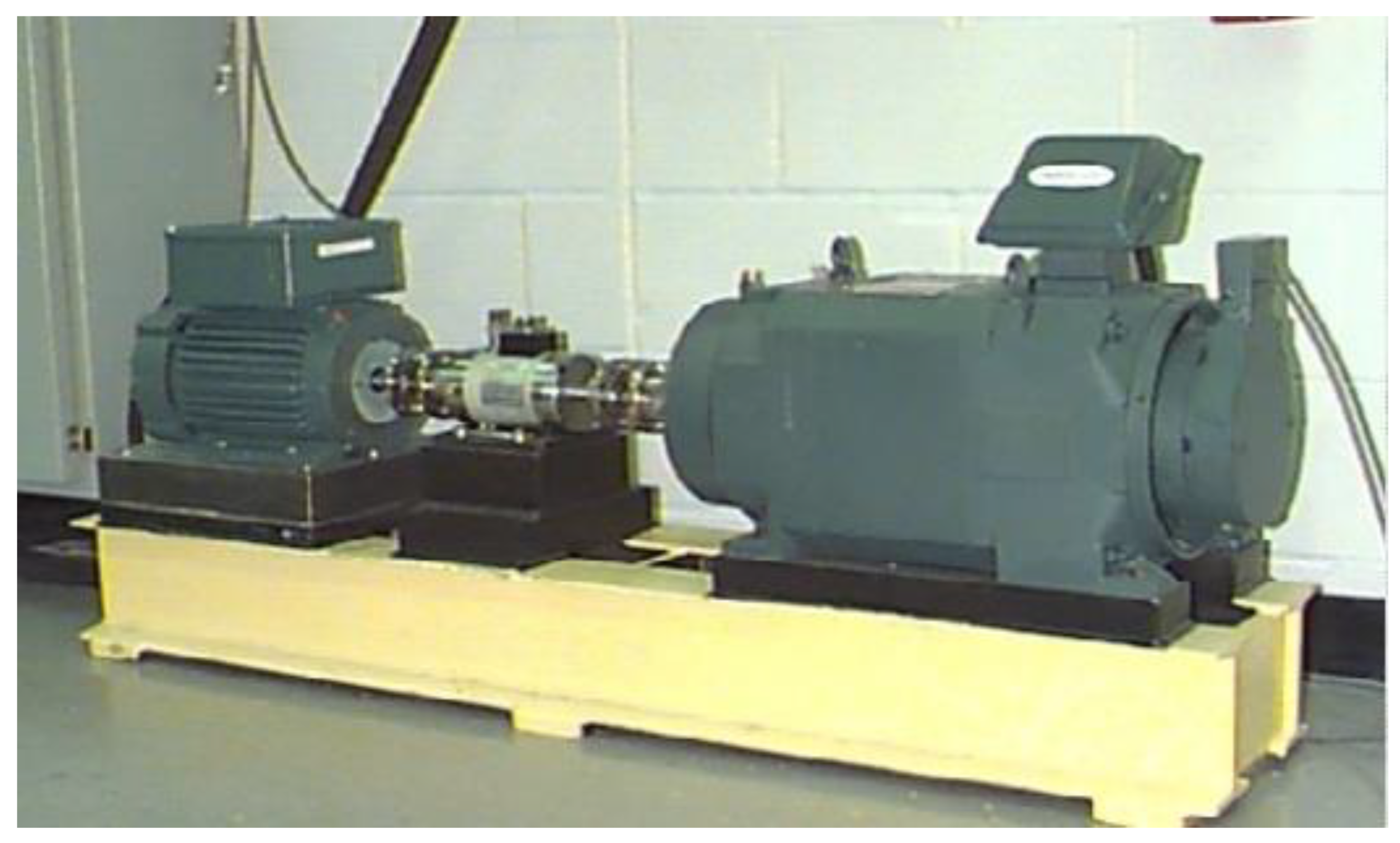
The experiment uses a computer equipped with Inter I5 4-core CPU, 16 GB memory, and 64-bit Windows 10 system to verify the superiority of the algorithm in this paper. Due to laboratory conditions, this article uses the vibration acceleration data of the Rolling Bearing Experimental Center of Western Reserve University for experimental verification, as shown in Figure 10.

Figure 10.
Signal acquisition platform for rolling bearing.
The fault is a single-point fault produced by an electric spark. Test the 6205SKF bearing, connect the bearing to the motor, and use the acceleration sensor to test the vibration signal at the fan end of the bearing. The motor speed is about 1700 r/min, and the sampling frequency is 12 kHz and 48 kHz. The specifications of the 6205SKF bearings are shown in Table 1.

Table 1.
6205SKF bearing parameters.
Each type of fault data includes four kinds of load conditions, and this experiment only selects the load of 0HP. In this case, the speed is 1797 r/min. The bearing fault frequency calculated according to formula (19) is shown in Table 2.

Table 2.
0HP fault frequency.
In the data set, there are only three types of single-point fault diameters for electric spark machining of 6205SKF bearings, so the corresponding fault types in this experiment are shown in Table 3.

Table 3.
Bearing fault characteristics defined in this paper.
When the load is 0HP under normal working conditions, the corresponding data set is 97. The vibration time-domain waveform of that data set optimized by this system is shown in Figure 11. According to Formula (14), the average value of the upper limit of normal vibration amplitude is calculated to be 0.098 mm/s2.

Figure 11.
Time-domain image of bearing under normal operating conditions.
Take the different fault data of the drive end with sampling frequency of 48 kHz, load 0 HP, and 6 o’clock direction of the outer race. Three data sets meet the requirements. Each data set contains at least 240,000 vibration data. Taking every 1200 vibration acceleration data as a complete cycle of sampling data, 200 data sets will be obtained. Randomly take 150 groups of minor, moderate, and serious faults as experimental data and record them as A150, B150, and C150, respectively. The remaining 50 groups of each data set are recorded as T150 as test data.
Step 1. Take the data in A150, B150, and C150 for optimization analysis using this system.
Step 2. Calculate the value of , according to Formula (17). After that, all values are normalized according to Formula (18) to obtain .
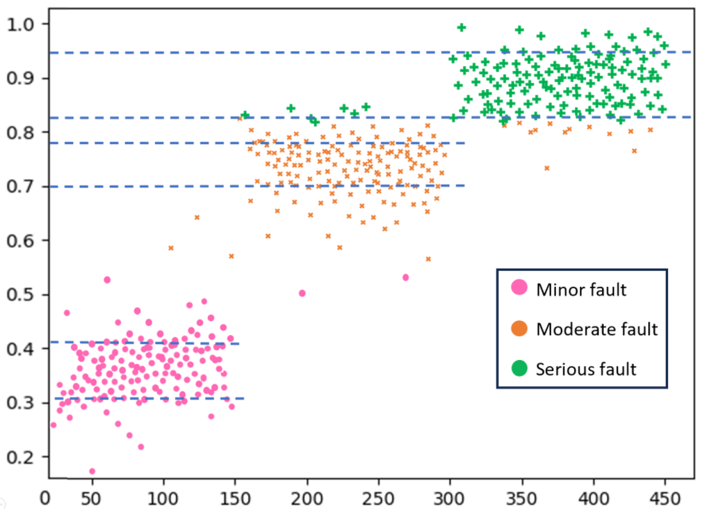
Step 3. To more intuitively see the scope of various types of faults, use this system to divide the normalized data into three categories, as shown in Figure 12.
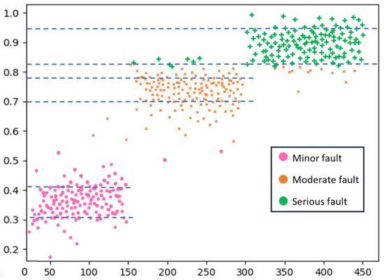
Figure 12.
The clustering results of this system.
Step 4. Determine the normalized range of the vibration amplitude of various faults, see Table 4.

Table 4.
Impulse indicators of various types of faults.
Step 5. This system converts the data obtained in Step 1 into frequency domain signals. Envelope analysis is performed to extract the low-frequency modulation signal in the high-frequency vibration signal, and then the power spectrum analysis is performed on each obtained low-frequency modulation signal. An individual example of power spectrum analysis is shown in Figure 13. Record the maximum multiplier of each group of data harmonics.

Figure 13.
Power spectrum of individual example data.
Step 6. Repeat Step 3 for . Obtain the normalized range of the harmonic frequency multiplication of various faults, see Table 5.

Table 5.
Harmonic frequency multiplication range of various faults.
Step 7. Combine the amplitude values in Table 5 with the harmonic frequency multiplication signal to construct fuzzy signal set , as shown in Equation (20).
Through the above steps, a diagnostic model of fault data fusion can be obtained. After that, the fault diagnosis can be performed, and the diagnosis result is the fault type set , as shown in Formula (21). Where is the target to be detected.
After the system is calibrated and stabilized, take any four sets of data from T150 for fault diagnosis. , , , . Then, . According to the maximum method, it is considered that has a minor fault. The fault diagnosis results of the four groups of data are shown in Table 6.

Table 6.
Fault diagnosis results.
Use this system to diagnose faults on the T150 data set, and the visualized results are shown in Figure 14.
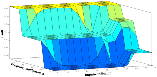
Figure 14.
Visualized results of fault diagnosis of T150 data set by this system.
The fuzzy signal fault diagnosis method proposed in this paper can determine the fault type through a simple set operation. Compared with other fault diagnosis methods, this process does not require a large amount of data as a basis. It calculates the fault attribute of the thing itself as the data and quickly identifies the fault without other complicated steps, making it easier and more efficient.
The LSTM network can extract more extensive feature signals, can effectively suppress the high-frequency noise in the vibration signal, and is often used in the fault diagnosis of rolling bearings. Choose an LSTM network with two layers and 128 neurons in each layer for comparison experiments. The A150, B150, and C150 data sets are used as training data, and T150 is used as test data. Suppose the number of correct recognition is and the total number of test samples is , then the correct identification rate is as shown in Formula (22).
With the T150 test data set, 500 experiments were performed, respectively. Similarly, the proposed method is compared with the latest neural network methods. The correct comparison result of the proposed method and the existing methods is shown in Figure 15. It can be seen from the results that the correct recognition rate of the proposed method is as high as 91.9%.
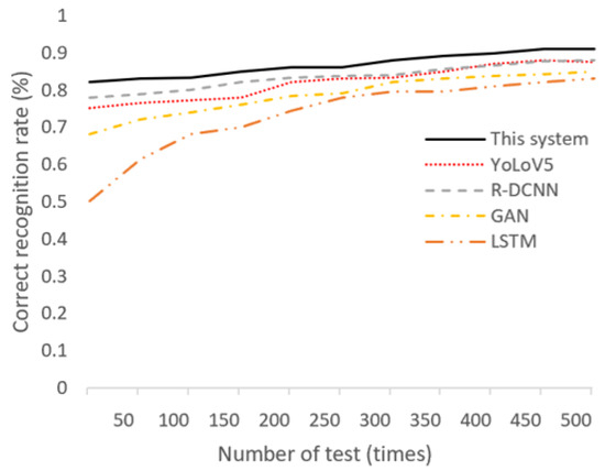
Figure 15.
Comparison of the correct recognition rate between proposed method and existing methods.
This method is not only more accurate than the existing network in terms of correct recognition rate but also significantly better than the existing network in terms of rapidity. Both tested the T150 data set, and the rapidity comparison is shown in Table 7.

Table 7.
Comprehensive comparison of the proposed method and existing methods.
6. Conclusions
Based on the theoretical basis of the operation of fuzzy sets, this paper defines fuzzy mapping with new connotative features. The fuzzy closeness vector function is defined as a method of fuzzy data processing. At the same time, based on the definition of the inner product and outer product of vectors, the definition of the inner product and outer product on the fuzzy set is given, and the fuzzy signal fault diagnosis method is discussed. Taking the key technology of fuzzy fault signal processing and fault diagnosis as the direction, this kind of novel, unique, and effective soft scientific method can analyze and process fuzzy fault signals. It can effectively and quickly realize fuzzy signal collection, processing, fault diagnosis, and decision making. It processes and diagnoses faults quickly and is closer to the natural attributes of things. The simulation results show that, compared with using the neural network alone, the average time consumption is reduced and the fault recognition accuracy rate is increased. The application potential of fuzzy set theory is huge, so scholars need to conduct in-depth research into many aspects in the future.
Author Contributions
Formal analysis, Z.F. and W.W.; Resources, Q.-E.W.; Data curation, Q.-E.W.; Writing—original draft, Z.F.; Writing—review & editing, Z.F., Q.-E.W., W.W. and S.W.; validation, S.W. All authors have read and agreed to the published version of the manuscript.
Funding
This work is supported by the Key Science and Technology Program of Henan Province (222102210084); Key Science and Technology Project of Henan Province University (23A413007).
Institutional Review Board Statement
Not applicable.
Informed Consent Statement
Not applicable.
Data Availability Statement
All data generated or analyzed during this study are included in this article. We do wish to share our raw data, and these data are original.
Conflicts of Interest
This manuscript has not been published and is not under consideration for publication elsewhere. We have no conflict of interest to disclose.
References
- Roy, S.S.; Dey, S.; Chatterjee, S. Autocorrelation aided random forest classifier based bearing fault detection framework. IEEE Sens. J. 2020, 20, 10792–10800. [Google Scholar] [CrossRef]
- Merizalde, Y.; Hernández-Callejo, L.; Duque-Pérez, O.; Alonso-Gómez, V. Diagnosis of wind turbine faults using generator current signature analysis: A review. J. Qual. Maint. Eng. 2019, 26, 431–458. [Google Scholar] [CrossRef]
- Wang, H.; Guo, Z.; Du, W. Diagnosis of rolling element bearing based on multifractal detrended fluctuation analyses and continuous hidden markov model. J. Mech. Sci. Technol. 2021, 35, 3313–3322. [Google Scholar] [CrossRef]
- Larizza, F.; Howard, C.Q.; Grainger, S. Defect size estimation in rolling element bearings with angled leading and trailing edges. Struct. Health Monit. 2021, 20, 1102–1116. [Google Scholar] [CrossRef]
- Bao, W.; Tu, X.; Hu, Y.; Li, F. Envelope spectrum l-kurtosis and its application for fault detection of rolling element bearings. IEEE Trans. Instrum. Meas. 2019, 69, 1993–2002. [Google Scholar] [CrossRef]
- Kumbhar, S.G.; Sudhagar, P.E.; Desavale, R.G. An overview of dynamic modeling of rolling-element bearings. Noise Vib. Worldw. 2021, 52, 3–18. [Google Scholar] [CrossRef]
- Zhang, J.; Wu, J.; Hu, B.; Tang, J. Intelligent fault diagnosis of rolling bearings using variational mode decomposition and self-organizing feature map. J. Vib. Control 2020, 26, 1886–1897. [Google Scholar] [CrossRef]
- Singh, P.; Harsha, S.P. Statistical and frequency analysis of vibrations signals of roller bearings using empirical mode decomposition. J. Multi-Body Dyn. 2019, 233, 856–870. [Google Scholar] [CrossRef]
- Li, H.; Liu, T.; Wu, X.; Chen, Q. Enhanced frequency band entropy method for fault feature extraction of rolling element bearings. IEEE Trans. Ind. Inform. 2019, 16, 5780–5791. [Google Scholar] [CrossRef]
- Gao, J.H.; Guo, M.F.; Xiang, S. Feature-clustering-based single-line-to-ground fault section location using auto-encoder and fuzzy C-means clustering in resonant grounding distribution systems. IET Gener. Transm. Distrib. 2021, 15, 938–949. [Google Scholar] [CrossRef]
- Babiker, A.; Yan, C.; Li, Q.; Meng, J.; Wu, L. Initial fault time estimation of rolling element bearing by backtracking strategy, improved VMD and infogram. J. Mech. Sci. Technol. 2021, 35, 425–437. [Google Scholar] [CrossRef]
- Li, J.; Wang, Y.; Zi, Y.; Jiang, S. A local weighted multi-instance multilabel network for fault diagnosis of rolling bearings using encoder signal. IEEE Trans. Instrum. Meas. 2020, 69, 8580–8589. [Google Scholar]
- Zhang, X.; Zhao, J.M.; Li, H.P.; Yang, R.F.; Teng, H.Z. Rolling bearings fault diagnosis under variable conditions using rcmfe and improved support vector machine. Int. J. Acoust. Vib. 2020, 25, 304–317. [Google Scholar] [CrossRef]
- Cui, M.; Wang, Y.; Lin, X.; Zhong, M. Fault diagnosis of rolling bearings based on an improved stack autoencoder and support vector machine. IEEE Sens. J. 2021, 21, 4927–4937. [Google Scholar] [CrossRef]
- Akpudo, U.; Hur, J.W. A deep learning approach to prognostics of rolling element bearings. Int. J. Integr. Eng. 2020, 12, 178–186. [Google Scholar]
- Tian, Z.; Ren, Y.; Wang, G. Short-term wind power prediction based on empirical mode decomposition and improved extreme learning machine. J. Electr. Eng. Technol. 2018, 13, 1841–1851. [Google Scholar]
- Wang, Y.J.; Ding, X.X.; Zeng, Q. Intelligent rolling bearing fault diagnosis via vision convnet. IEEE Sens. J. 2021, 21, 6600–6609. [Google Scholar] [CrossRef]
- Jiao, J.Y.; Zhao, M.; Lin, J. Unsupervised adversarial adaptation network for intelligent fault diagnosis. IEEE Trans. Ind. Electron. 2020, 67, 9904–9913. [Google Scholar] [CrossRef]
- Pu, H.; Zhang, K.; An, Y. Restricted Sparse Networks for Rolling Bearing Fault Diagnosis. IEEE Trans. Ind. Inform. 2023, 19, 11139–11149. [Google Scholar] [CrossRef]
- Jiang, H.; Lu, H.; Zhou, J.; Liu, M. Fault Diagnosis of Rolling Bearings in VMD and GWO-ELM. In Proceedings of the 2022 3rd International Conference on Smart Grid and Energy Engineering (SGEE 2022), Nanjing, China, 25–27 November 2022; Volume 2496, pp. 12–13. [Google Scholar]
- Jandaghi, E.; Chen, X.T.; Yuan, C.Z. Motion Dynamics Modeling and Fault Detection of a Soft Trunk Robot. IEEE ASME Int. Conf. Adv. Intell. Mechatron. 2023, 1, 1324–1329. [Google Scholar]
- Yang, H.Q.; Wang, Z.H.; Song, K.L. A new hybrid grey wolf optimizer-feature weighted-multiple kernel-support vector regression technique to predict TBM performance. Eng. Comput. 2022, 38, 2469–2485. [Google Scholar] [CrossRef]
- Yang, H.Q.; Xing, S.G.; Wang, Q.; Li, Z. Model test on the entrainment phenomenon and energy conversion mechanism of flow-like landslides. Eng. Geol. 2018, 239, 119–125. [Google Scholar] [CrossRef]
- Jafarlou, M.; Ebadati, O.M.E.; Naderi, H. Improving Fuzzy-Logic based Map-Matching Method with Trajectory Stay-Point Detection. Lect. Notes Eng. Comput. Sci. 2023, 2245, 48–57. [Google Scholar]
- Darabi, N.; Tayebati, S.; Sureshkumar, S.; Ravi, S.; Tulabandhula, T.; Trivedi, A. STARNet: Sensor Trustworthiness and Anomaly Recognition via Approximated Likelihood Regret for Robust Edge Autonomy. arXiv 2023, arXiv:2309.11006. [Google Scholar]
- Haj Mohamad, T.; Nataraj, C. Fault identification and severity analysis of rolling element bearings using phase space topology. J. Vib. Control 2021, 27, 295–310. [Google Scholar] [CrossRef]
- Akpudo, U.E.; Hur, J.W. A feature fusion-based prognostics approach for rolling element bearings. J. Mech. Sci. Technol. 2020, 34, 4025–4035. [Google Scholar] [CrossRef]
Disclaimer/Publisher’s Note: The statements, opinions and data contained in all publications are solely those of the individual author(s) and contributor(s) and not of MDPI and/or the editor(s). MDPI and/or the editor(s) disclaim responsibility for any injury to people or property resulting from any ideas, methods, instructions or products referred to in the content. |
© 2023 by the authors. Licensee MDPI, Basel, Switzerland. This article is an open access article distributed under the terms and conditions of the Creative Commons Attribution (CC BY) license (https://creativecommons.org/licenses/by/4.0/).

