
Research on Improved Fault Detection Method of Rolling Bearing Based on Signal Feature Fusion Technology

Abstract
:1. Introduction
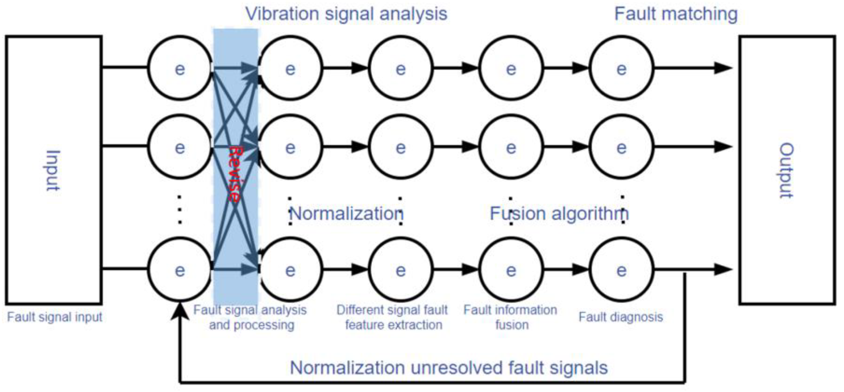
2. Fuzzy Signal Analysis on Fault Diagnosis System
3. Fuzzy Fault Diagnosis Method
3.1. Fuzzy Mapping
3.2. Fuzzy Signal Processing Algorithm
3.3. Judgment Principle for Fault Diagnosis
- (1)
- Maximum method
- (2)
- Minimum difference method
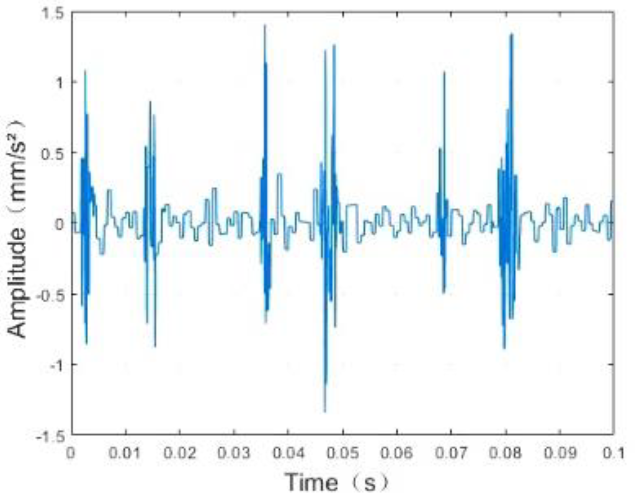
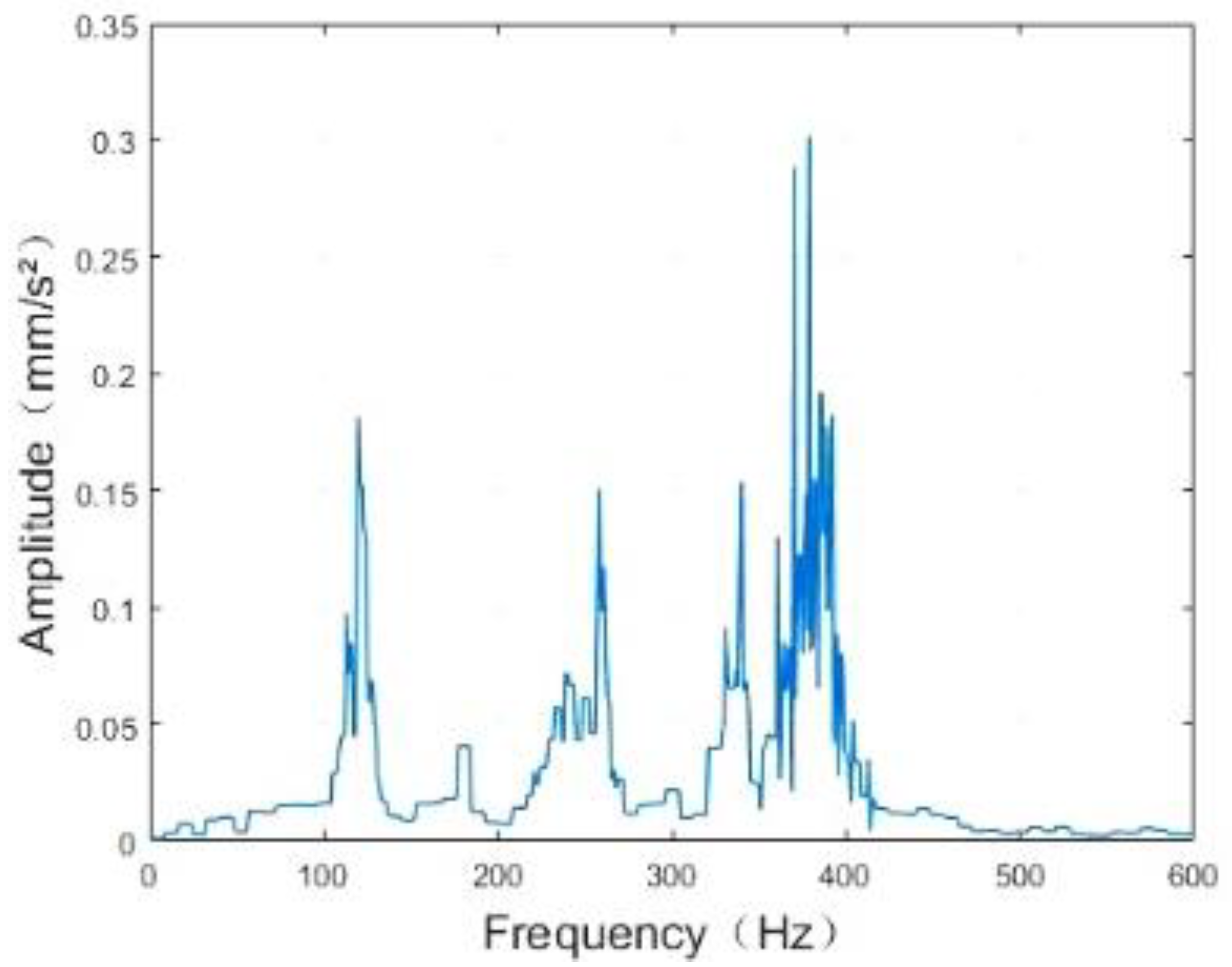
4. Vibration Signal Analysis of Rolling Bearing
5. Comparison of the Proposed Method with the Existing Method
6. Conclusions
Author Contributions
Funding
Institutional Review Board Statement
Informed Consent Statement
Data Availability Statement
Conflicts of Interest
References
- Roy, S.S.; Dey, S.; Chatterjee, S. Autocorrelation aided random forest classifier based bearing fault detection framework. IEEE Sens. J. 2020, 20, 10792–10800. [Google Scholar] [CrossRef]
- Merizalde, Y.; Hernández-Callejo, L.; Duque-Pérez, O.; Alonso-Gómez, V. Diagnosis of wind turbine faults using generator current signature analysis: A review. J. Qual. Maint. Eng. 2019, 26, 431–458. [Google Scholar] [CrossRef]
- Wang, H.; Guo, Z.; Du, W. Diagnosis of rolling element bearing based on multifractal detrended fluctuation analyses and continuous hidden markov model. J. Mech. Sci. Technol. 2021, 35, 3313–3322. [Google Scholar] [CrossRef]
- Larizza, F.; Howard, C.Q.; Grainger, S. Defect size estimation in rolling element bearings with angled leading and trailing edges. Struct. Health Monit. 2021, 20, 1102–1116. [Google Scholar] [CrossRef]
- Bao, W.; Tu, X.; Hu, Y.; Li, F. Envelope spectrum l-kurtosis and its application for fault detection of rolling element bearings. IEEE Trans. Instrum. Meas. 2019, 69, 1993–2002. [Google Scholar] [CrossRef]
- Kumbhar, S.G.; Sudhagar, P.E.; Desavale, R.G. An overview of dynamic modeling of rolling-element bearings. Noise Vib. Worldw. 2021, 52, 3–18. [Google Scholar] [CrossRef]
- Zhang, J.; Wu, J.; Hu, B.; Tang, J. Intelligent fault diagnosis of rolling bearings using variational mode decomposition and self-organizing feature map. J. Vib. Control 2020, 26, 1886–1897. [Google Scholar] [CrossRef]
- Singh, P.; Harsha, S.P. Statistical and frequency analysis of vibrations signals of roller bearings using empirical mode decomposition. J. Multi-Body Dyn. 2019, 233, 856–870. [Google Scholar] [CrossRef]
- Li, H.; Liu, T.; Wu, X.; Chen, Q. Enhanced frequency band entropy method for fault feature extraction of rolling element bearings. IEEE Trans. Ind. Inform. 2019, 16, 5780–5791. [Google Scholar] [CrossRef]
- Gao, J.H.; Guo, M.F.; Xiang, S. Feature-clustering-based single-line-to-ground fault section location using auto-encoder and fuzzy C-means clustering in resonant grounding distribution systems. IET Gener. Transm. Distrib. 2021, 15, 938–949. [Google Scholar] [CrossRef]
- Babiker, A.; Yan, C.; Li, Q.; Meng, J.; Wu, L. Initial fault time estimation of rolling element bearing by backtracking strategy, improved VMD and infogram. J. Mech. Sci. Technol. 2021, 35, 425–437. [Google Scholar] [CrossRef]
- Li, J.; Wang, Y.; Zi, Y.; Jiang, S. A local weighted multi-instance multilabel network for fault diagnosis of rolling bearings using encoder signal. IEEE Trans. Instrum. Meas. 2020, 69, 8580–8589. [Google Scholar]
- Zhang, X.; Zhao, J.M.; Li, H.P.; Yang, R.F.; Teng, H.Z. Rolling bearings fault diagnosis under variable conditions using rcmfe and improved support vector machine. Int. J. Acoust. Vib. 2020, 25, 304–317. [Google Scholar] [CrossRef]
- Cui, M.; Wang, Y.; Lin, X.; Zhong, M. Fault diagnosis of rolling bearings based on an improved stack autoencoder and support vector machine. IEEE Sens. J. 2021, 21, 4927–4937. [Google Scholar] [CrossRef]
- Akpudo, U.; Hur, J.W. A deep learning approach to prognostics of rolling element bearings. Int. J. Integr. Eng. 2020, 12, 178–186. [Google Scholar]
- Tian, Z.; Ren, Y.; Wang, G. Short-term wind power prediction based on empirical mode decomposition and improved extreme learning machine. J. Electr. Eng. Technol. 2018, 13, 1841–1851. [Google Scholar]
- Wang, Y.J.; Ding, X.X.; Zeng, Q. Intelligent rolling bearing fault diagnosis via vision convnet. IEEE Sens. J. 2021, 21, 6600–6609. [Google Scholar] [CrossRef]
- Jiao, J.Y.; Zhao, M.; Lin, J. Unsupervised adversarial adaptation network for intelligent fault diagnosis. IEEE Trans. Ind. Electron. 2020, 67, 9904–9913. [Google Scholar] [CrossRef]
- Pu, H.; Zhang, K.; An, Y. Restricted Sparse Networks for Rolling Bearing Fault Diagnosis. IEEE Trans. Ind. Inform. 2023, 19, 11139–11149. [Google Scholar] [CrossRef]
- Jiang, H.; Lu, H.; Zhou, J.; Liu, M. Fault Diagnosis of Rolling Bearings in VMD and GWO-ELM. In Proceedings of the 2022 3rd International Conference on Smart Grid and Energy Engineering (SGEE 2022), Nanjing, China, 25–27 November 2022; Volume 2496, pp. 12–13. [Google Scholar]
- Jandaghi, E.; Chen, X.T.; Yuan, C.Z. Motion Dynamics Modeling and Fault Detection of a Soft Trunk Robot. IEEE ASME Int. Conf. Adv. Intell. Mechatron. 2023, 1, 1324–1329. [Google Scholar]
- Yang, H.Q.; Wang, Z.H.; Song, K.L. A new hybrid grey wolf optimizer-feature weighted-multiple kernel-support vector regression technique to predict TBM performance. Eng. Comput. 2022, 38, 2469–2485. [Google Scholar] [CrossRef]
- Yang, H.Q.; Xing, S.G.; Wang, Q.; Li, Z. Model test on the entrainment phenomenon and energy conversion mechanism of flow-like landslides. Eng. Geol. 2018, 239, 119–125. [Google Scholar] [CrossRef]
- Jafarlou, M.; Ebadati, O.M.E.; Naderi, H. Improving Fuzzy-Logic based Map-Matching Method with Trajectory Stay-Point Detection. Lect. Notes Eng. Comput. Sci. 2023, 2245, 48–57. [Google Scholar]
- Darabi, N.; Tayebati, S.; Sureshkumar, S.; Ravi, S.; Tulabandhula, T.; Trivedi, A. STARNet: Sensor Trustworthiness and Anomaly Recognition via Approximated Likelihood Regret for Robust Edge Autonomy. arXiv 2023, arXiv:2309.11006. [Google Scholar]
- Haj Mohamad, T.; Nataraj, C. Fault identification and severity analysis of rolling element bearings using phase space topology. J. Vib. Control 2021, 27, 295–310. [Google Scholar] [CrossRef]
- Akpudo, U.E.; Hur, J.W. A feature fusion-based prognostics approach for rolling element bearings. J. Mech. Sci. Technol. 2020, 34, 4025–4035. [Google Scholar] [CrossRef]


| Inner Race Diameter | Outer Race Diameter | Thickness | Ball Diameter | Pitch Diameter | Number of Rolling Elements |
|---|---|---|---|---|---|
| 25 mm | 52 mm | 15 mm | 7.94 mm | 39.04 mm | 9 |
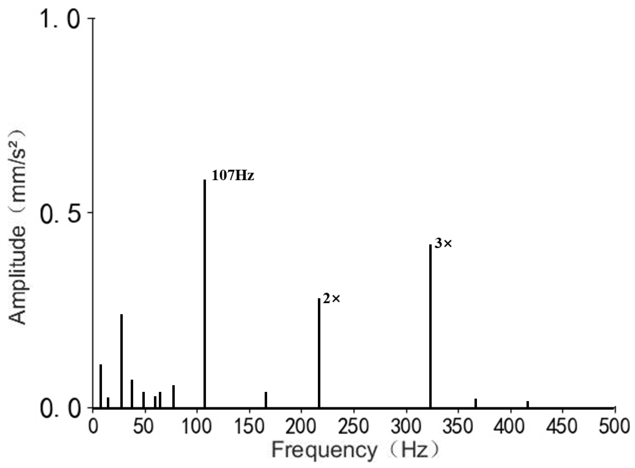
| Outer Race Fault | Inner Race Fault | Ball Fault |
|---|---|---|
| 107 Hz | 162 Hz | 141 Hz |
| Fault Type | Fault Diameter |
|---|---|
| Minor fault | 0.18 mm |
| Moderate fault | 0.36 mm |
| Serious fault | 0.53 mm |
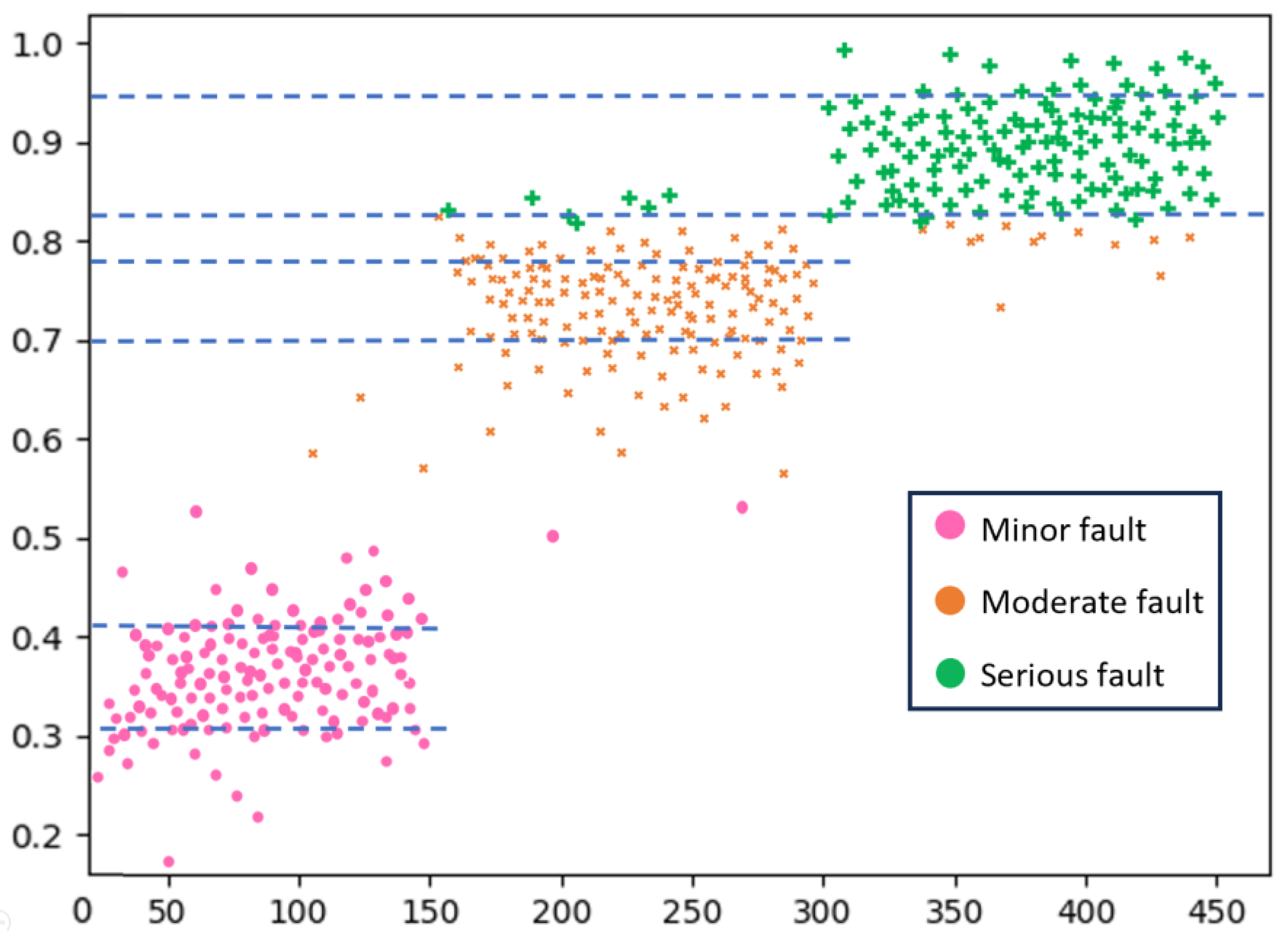
| Fault Type | Ambiguous Range of Impulse Indicator |
|---|---|
| Minor fault | 0.31–0.41 |
| Moderate fault | 0.70–0.78 |
| Serious fault | 0.83–0.95 |
| Fault Type | Ambiguous Range of Harmonic Frequency Multiplication |
|---|---|
| Minor fault | 0.10–0.30 |
| Moderate fault | 0.40–0.60 |
| Serious fault | 0.70–0.90 |
| Detection Target | Impulse Indicator | Frequency Multiplication | Fault Type |
|---|---|---|---|
| T1 | 0.24–0.36 | 0.10–0.30 | Minor fault |
| T2 | 0.74–0.86 | 0.40–0.60 | Serious fault |
| T3 | 0.66–0.76 | 0.40–0.60 | Moderate fault |
| T4 | 0.78–0.92 | 0.70–0.90 | Serious fault |
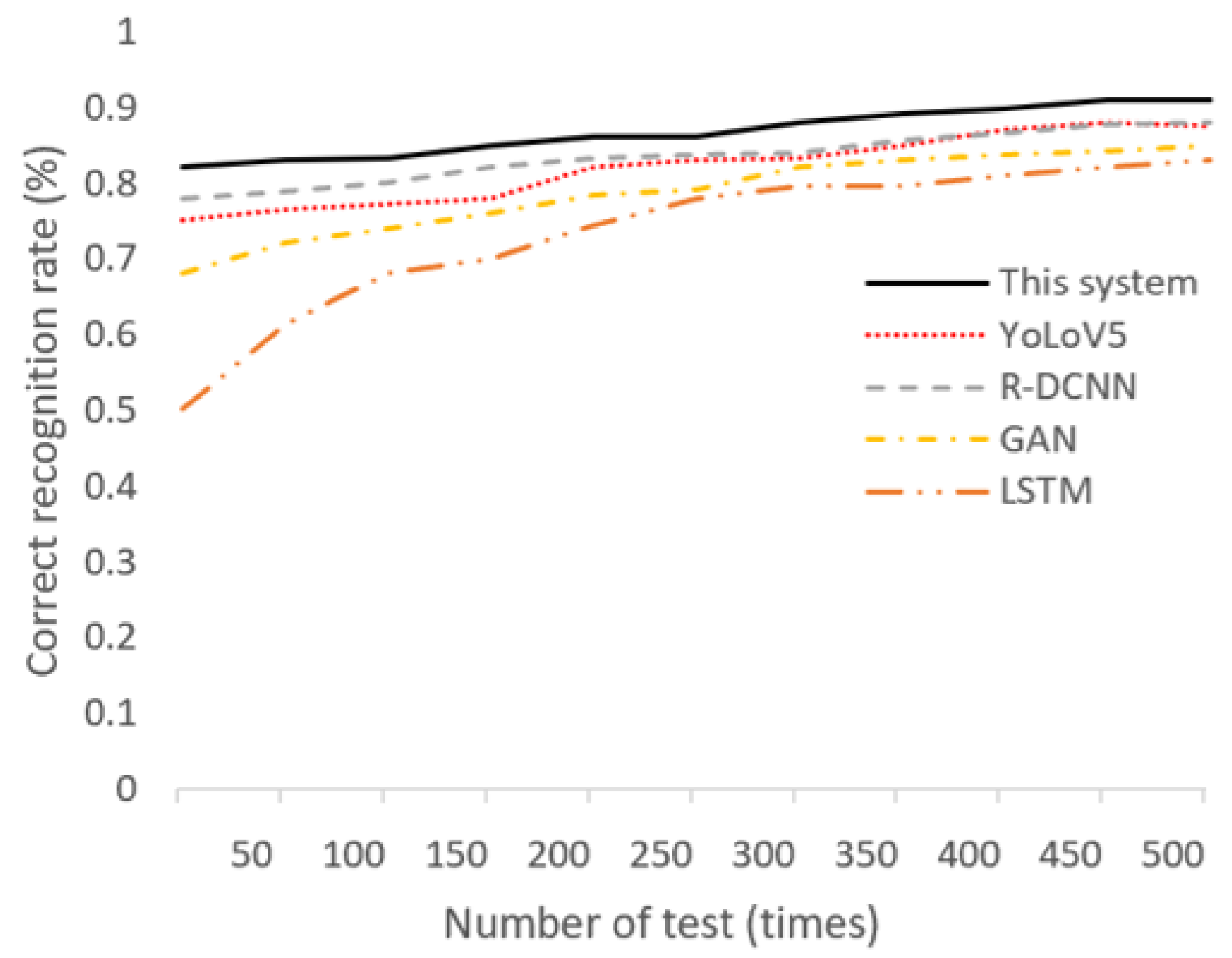
| Accuracy Rate (%) | Time Consuming (s) | Anti-Noise Property | |
|---|---|---|---|
| This system | 91.9 | 0.012 | Strong |
| YoLoV5 | 90.1 | 0.182 | Less strong |
| R-DCNN | 90.8 | 0.125 | Weak |
| GAN | 88.9 | 0.213 | Less strong |
| LSTM | 86.5 | 0.894 | Weak |
Disclaimer/Publisher’s Note: The statements, opinions and data contained in all publications are solely those of the individual author(s) and contributor(s) and not of MDPI and/or the editor(s). MDPI and/or the editor(s) disclaim responsibility for any injury to people or property resulting from any ideas, methods, instructions or products referred to in the content. |
© 2023 by the authors. Licensee MDPI, Basel, Switzerland. This article is an open access article distributed under the terms and conditions of the Creative Commons Attribution (CC BY) license (https://creativecommons.org/licenses/by/4.0/).
Share and Cite
Fang, Z.; Wu, Q.-E.; Wang, W.; Wu, S. Research on Improved Fault Detection Method of Rolling Bearing Based on Signal Feature Fusion Technology. Appl. Sci. 2023, 13, 12987. https://doi.org/10.3390/app132412987
Fang Z, Wu Q-E, Wang W, Wu S. Research on Improved Fault Detection Method of Rolling Bearing Based on Signal Feature Fusion Technology. Applied Sciences. 2023; 13(24):12987. https://doi.org/10.3390/app132412987
Chicago/Turabian StyleFang, Zhenggaoyuan, Qing-E Wu, Wenjing Wang, and Shuyan Wu. 2023. "Research on Improved Fault Detection Method of Rolling Bearing Based on Signal Feature Fusion Technology" Applied Sciences 13, no. 24: 12987. https://doi.org/10.3390/app132412987