Improved Computer Vision Framework for Mesoscale Simulation of Xiyu Conglomerate Using the Discrete Element Method

Abstract

The complex mechanical characteristics of the Xiyu conglomerate significantly influence the resistance and deformation features of its caverns’ surrounding rock, thereby constraining the construction of related water diversion tunnels. This paper introduces an improved SegFormer framework developed for the detection of mesoscale geomaterial structures. Computerized tomography (CT) scan images of the Xiyu conglomerate were employed to establish a high-precision numerical model. From the results of segmentation, the proposed algorithm outperformed UNet, HRNet, and the original SegFormer neural network. The segmentation results were used to calculate the porosity, and biaxial compression numerical simulation experiments based on the real structure were carried out using the particle flow code (PFC). We observed the failure process of the model and obtained the shear strength of the Xiyu conglomerate. We explored the causes and influencing factors of the anisotropy of the Xiyu conglomerate from the microstructure perspective and provide a micro-observation basis for establishing an anisotropic mechanical model.

1. Introduction

The Xiyu Formation, one of the most important and widely cited late Cenozoic strata in western China, refers to a set of dark gray or deep gray, massively thick, blocky conglomerate deposits that are widely distributed in the foothill zones of the Tianshan and Kunlun Mountains [1]. The thickness of the Xiyu conglomerate varies from tens of meters to several kilometers, with an average thickness of about 2000 m [2]. Due to its complex material composition and special structure, the Xiyu conglomerate has characteristics such as poor cementation, low mechanical strength, and softening when encountering water [3]. The resistance and deformation characteristics of the surrounding rock in the karst caves have become one of the key issues restricting the scientific design of related water diversion tunnel projects in this area [4]. In addition, rock slopes formed by the Xiyu conglomerate are prone to erosion at the slope toe, posing severe challenges to water conservancy and hydropower engineering construction in this area [5].

Currently, the existing failure models inadequately explain the mechanical properties of the Xiyu conglomerate, restricting the effectiveness of conventional evaluation methods in analyzing the stability of the Xiyu conglomerate’s slopes and tunnels. Qin [6] used a finite difference method to conduct numerical simulation experiments on the softening failure mechanism of the high slopes and slope toes of the Xiyu conglomerate and found that there was a significant difference between the simulation results and the observed slope failure phenomena. Wang et al. [7] analyzed the elastic resistance coefficient of the tunnels’ surrounding rock using an inversion method and calculated that there was a gap between the elastic resistance coefficient of the surrounding rock around the tunnel and the actual deformation resistance characteristics of the surrounding rock. Li et al. [8] studied the softening failure mechanism of the high slope toes of the Xiyu conglomerate using a range analysis method and analyzed the influence of the slope angle and other sensitivity factors on the stability of the high slopes, but this method cannot fully consider the influence of other factors, such as the mechanical properties of the Xiyu conglomerate, on stability.

In the field of characterizing the microstructure of heterogeneous material, with the widespread application and development of computer science and digital images, the coupling method of digital image processing and numerical simulation makes it possible to analyze the micromechanical behavior. This method is of great significance for studying the mechanical properties of heterogeneous materials [9]. Yang et al. [10] reconstructed non-homogeneous models, such as a silicate cement and asphalt mixture, based on real images and analyzed the advantages and disadvantages of image-based models and computer-generated models. Ali Abdulqader et al. [11] developed the StereoDIC system for detecting internal defects. This system was successfully applied in uniaxial compression tests of rock cores, suggesting its potential use in estimating material properties. Woodman et al. [12] utilized a coupled discrete element method (DEM) and grain-based modeling (GBM) simulations to accurately represent the microstructure of laboratory specimens. This approach allowed them to study the effects of thermo-mechanical loading on fine-grained sandstone in a detailed and precise manner. Yu et al. [13] successfully estimated the porosity of sedimentary rocks by using digital image analysis methods and pore and crack analysis systems (PCAS). Qian et al. [14] modified an automatic deep learning-based segmentation algorithm for scanning electron microscopy (SEM) images of cement paste. This enhanced approach has enabled the precise examination of the irregularity and roundness of unhydrated cement particles, as dictated by the segmentation results.

With the advancement of numerical simulation theory, the micromechanical properties of rocks can be studied using this technology [15,16]. Numerical simulations encompass three types of methods: continuous, discontinuous, and hybrid continuum–discontinuum [17]. Discontinuous methods, such as the DEM, are often favored in numerical simulations of heterogeneous materials due to their ability to explicitly consider microstructures and simulate complex fracture behaviors [18,19,20]. Based on the contact type, DEMs can be divided into two types. The first type is represented by the UDEC (Universal Distinct Element Code). It handles various contact types, including face–face, face–vertex, and vertex–vertex, necessitating complex algorithms [21,22]. Another type is the PFC, where the contact is simpler and only one contact appears between two practices [18,23,24]. Notably, the PFC offers higher computational efficiency, which is why it was chosen for this study; however, it is computationally slower due to complex contact detection, and it has certain limitations in dealing with continuum analysis [25].

In this study, a computer vision framework was modified to establish the DEM model with real geomaterial structures, and a biaxial compression numerical simulation experiment was conducted by the spherical DEM software PFC to investigate the mechanical properties of the Xiyu conglomerate. This study successfully demonstrates that the approach can effectively segment the CT images of the rock and precisely simulate its mechanical behavior under various loading conditions. The deep learning-based segmentation model employed in this research outperforms the previous edge detection techniques in segmenting the mesoscale structures of geomaterials. This advancement enables more accurate mesoscale simulation and facilitates further investigation of the anisotropy of heterogeneous materials based on this study.

2. Method

The collective Xiyu conglomerate was subjected to CT scanning. After three-dimensional reconstruction of the obtained CT images, slicing was performed. Subsequently, different components within the rock were labeled. A dataset for training and validation of the deep learning model was generated. Afterwards, instance segmentation of other regions was performed using the trained model. The porosity of the rock was calculated, and the boundaries of each component were segmented. A high-precision numerical simulation model was generated using the segmented images. Two-dimensional biaxial compression tests were conducted. This section will provide a detailed discussion of these steps.

2.1. Improvements and Training of the SegFormer Network

2.1.1. Data Preparation

The samples utilized in this study were extracted from the Xinjiang region, specifically, from the Xiyu conglomerate rocks, with sample dimensions of 50 mm × 100 mm. Due to the limited data and unfavorable training conditions for the neural network with large images, image cropping became necessary. To preserve the original aspect ratio, the initial images underwent interpolation to a size of 4096 × 3584 pixels. Subsequently, non-overlapping cropping was applied, reducing the size to 512 × 512 pixels, with a cropping stride of 512 × 512 pixels. This enabled the creation of 56 (8 × 7) cropped images from each original image.

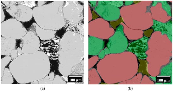
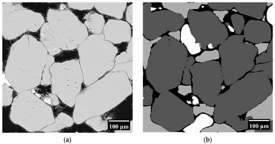
The gravel, pore, and matrix of the rocks were identified and labeled as regions of interest (ROI) using LabelMe, a graphical tool for manual image annotation [26]. These regions, depicted in Figure 1, are also referred to as instances. In this study, the ROIs were manually labeled, a common approach in supervised learning. Manual annotation, while highly accurate, has the drawback of being time-consuming and labor-intensive. The distinct colors in Figure 1 denote different ROI instances.

2.1.2. Constructing Networks

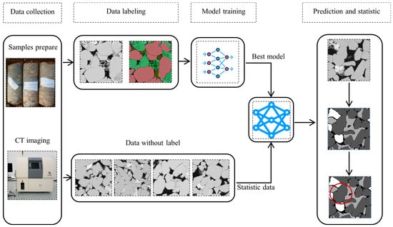
The network construction framework for this study is illustrated in Figure 2. Semantic segmentation, a highly popular and crucial aspect of deep learning in computer vision, involves labeling each pixel in an image with its corresponding semantic class, achieving fine-grained segmentation and comprehension of the image. Standard datasets like COCO (common objects in context) and Cityscapes are extensively employed for semantic segmentation tasks [27,28]. These datasets furnish numerous images with pixel-level labels that are utilized for training and evaluating the performance of semantic segmentation models. Many deep learning algorithms are designed to address semantic segmentation tasks akin to the aforementioned standard datasets. However, everyday photos exhibit notable differences from CT images:

• CT images encapsulate high-resolution internal structural information, enabling applications in rock classification and mineral composition analysis. They excel in capturing subtle structures and details at the microscale, contributing to their larger dimensions.
• Owing to specific domain constraints, CT images typically possess a smaller overall data volume compared to extensive existing datasets. Moreover, data diversity may be relatively low, and the distinctions between labels might not be as apparent. Traditional algorithms may struggle to predict effectively in this context.
• In the research process, it is essential to output the porosity of specified regions based on CT images. This necessitates achieving more comprehensive segmentation on the boundaries of these regions and the capability to model long distances.

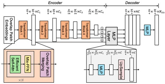
Considering points 2 and 3, along with additional considerations related to image texture, the Transformer architecture was selected. It is crucial to account for the impact of features at different scales and determine how to amalgamate these diverse features. The decoder of SegFormer incorporates this functionality. The fundamental concept of this algorithm involves integrating the self-attention mechanism of Transformer into the semantic segmentation task, empowering the model to establish relationships between different pixels and comprehend the global and local structure of the image [29,30]. In contrast to traditional convolutional neural network (CNN)-based segmentation methods, SegFormer harnesses Transformer’s ability to capture long-range dependencies between pixels, proving highly effective in addressing intricate segmentation challenges. The network architecture of SegFormer, comprising the hierarchical Transformer encoder and lightweight ALL-MLP decoder modules, is shown in Figure 3.

• The hierarchical Transformer encoder functions as the core network in the SegFormer model. It is tasked with extracting features from the input image and transmitting these features to the segmentation decoder. Its purpose is to capture features at various scales within the image and integrate global contextual information, thereby improving segmentation performance.
• The objective of this module is to generate CNN-like multi-level features when given an input image. These features offer high-resolution coarse features and low-resolution fine-grained features, typically enhancing the performance of semantic segmentation. More precisely, for an input image with a resolution of $H\times W\times 3$, patch merging is performed to yield a hierarchical feature map $F_i$, with a resolution calculated as follows:

  $$\frac{H}{2^{i+1}}\times \frac{W}{2^{i+1}}\times C_i,i=\left\{\mathrm{1,2},\mathrm{3,4}\right\},C_{i+1}>C_i$$

  (1)
• Overlapped patch merging is employed to reduce the size of the feature maps while simultaneously increasing the number of channels.
• The self-attention layer in the encoder represents the most computationally demanding component. To mitigate computational complexity, a reduction ratio (RRR) is applied to decrease the length of the sequence:

  $$\widehat{K}=\mathrm{Reshape}\left(\frac{N}{R},C·R\right)\left(K\right)$$

  (2)

  $$\mathrm{K}=\mathrm{Linear}\left(C·R,C\right)\left(\widehat{K}\right)$$

  (3)

  where $K$ is the sequence to be reduced, Reshape $(\frac{N}{R},C·R)\left(K\right)$ refers to reshape $K$ to the one with a shape of $\frac{N}{R}$ × ($C$ · $R$), and Linear $(C_{in};C_{out})(·)$ refers to a linear layer taking a $C_{in}$-dimensional tensor as input and generating a $C_{out}$-dimensional tensor as output [31].
• Mix-FFN: enhancing transformer layers with positional information. The Mix-FFN structure enhances Transformer layers by integrating positional information. This is accomplished by incorporating a 3 × 3 convolutional layer and an MLP layer into the FFN:

  $${\mathbf{x}}_{out}={\mathrm{M}\mathrm{L}\mathrm{P}\left(\mathrm{G}\mathrm{E}\mathrm{L}\mathrm{U}\right(\mathrm{C}\mathrm{o}\mathrm{n}\mathrm{v}}_{3\times 3}\left({\mathrm{M}\mathrm{L}\mathrm{P}(\mathbf{x}}_{in}\right)\left)\right))+{\mathbf{x}}_{in},$$

  (4)
• Lightweight ALL-MLP decoder: The lightweight ALL-MLP decoder serves as the segmentation decoder in the SegFormer model. Its primary objective is to transform the feature maps extracted by the encoder into pixel-level semantic segmentation predictions. This is accomplished through multi-scale feature fusion and upsampling to produce the final semantic segmentation mask. An essential rationale for SegFormer’s use of MLP in the decoder lies in the larger receptive field of Transformers compared to CNNs. The decoding process can be summarized as follows:

• Multiple hierarchical features are fed into an MLP layer to standardize the channel dimension;
• Feature maps are upsampled to 1/4 of the original image size and subsequently concatenated;
• A single MLP layer aggregates the feature channels;
• The predicted segmentation mask is outputted with a resolution calculated as follows:

$$\frac{H}{4}\times \frac{W}{4}\times N_{cls}$$

(5)

where $N_{cls}$ is the number of categories.

The decoder is formulated as follows:

$${\widehat{F}}_i=Linear\left(C_i,C\right)\left(F_i\right),\forall i$$

(6)

$${\widehat{F}}_i=Upsample\left(\frac{W}{4}\times \frac{W}{4}\right)\left({\widehat{F}}_i\right),\forall i$$

(7)

$$F=\mathrm{L}\mathrm{i}\mathrm{n}\mathrm{e}\mathrm{a}\mathrm{r}\left(4C,C\right)\left(\mathrm{C}\mathrm{o}\mathrm{n}\mathrm{c}\mathrm{a}\mathrm{t}\left({\widehat{F}}_i\right)\right),\forall i$$

(8)

$$M=\mathrm{L}\mathrm{i}\mathrm{n}\mathrm{e}\mathrm{a}\mathrm{r}\left(C,N_{cls}\right)\left(F\right),$$

(9)

where $M$ refers to the predicted mask and Linear($C_{in}$; $C_{out}$)(·) refers to a linear layer with $C_{in}$ and $C_{out}$ as the input and output vector dimensions, respectively [31].

In this study, enhancements have been made to the decoder of the SegFormer model. The original decoder concatenated features from different scales, overlooking the inherent differences in these features across the scales. Lower-level features typically capture structural and textural characteristics, while higher-level features focus more on semantic representation. In contrast to other methods, the improved algorithm prioritizes the complementarity between these two types of features. Unet and HRNet, as network architectures in deep learning, have been extensively applied in image segmentation tasks, with the goal of labeling each pixel in an image with a specific semantic category for precise image segmentation [32,33]. These models underscore the significance of multi-scale features for better information capture at different sizes and levels, thereby enhancing segmentation performance. The segmentation results of UNet, HRNet, the original SegFormer, and the modified SegFormer were compared.

UNet is a deep learning neural network architecture employed for image segmentation tasks. Its name is derived from its U-shaped network structure. A key feature is the combination of an encoder and a decoder, utilized for pixel-level image segmentation tasks. This facilitates the assignment of each pixel in the input image to a specific semantic category, achieving semantic segmentation at the pixel level. The structure of UNet, encompassing the encoding–decoding structure and the use of skip connections, has served as inspiration for many other network architectures, such as SegNet and PSPNet. Initially applied in the field of medical image segmentation, such as segmenting tissue structures in MRI and CT images, UNet has evolved into a widely employed algorithm in practical applications, including geotechnical engineering [34].

HRNet aims to uphold feature propagation at multiple resolutions for the improved capture of details and contextual information in images, thus enhancing segmentation performance. Its core idea involves preserving feature maps at multiple resolutions, addressing the resolution loss issue in traditional convolutional neural networks. HRNet is especially adept at handling fine-grained objects, retaining high-resolution information for better discrimination, and localization of small objects or intricate structures. The model’s multi-branch structure facilitates information capture at different scales, augmenting the model’s comprehension of object context and overall structure. Detailed network configurations for HRNet can be found in the literature [35].

2.1.3. Improvements to SegFormer

While the SegFormer model performs feature fusion across different scales, the fusion process might not adequately account for differences between these features in certain scenarios, leading to suboptimal performance. The SegFormer model utilizes the hierarchical Transformer decoder and the lightweight ALL-MLP decoder in the decoder module for fusing features at different scales. Although these methods theoretically capture the relationship between features at different scales, in practice, the model’s design and parameter settings may not fully address the distinctions between these features.

The hierarchical Transformer decoder is employed to model features at different scales, but the Transformer module may not effectively handle spatial differences in some cases. Additionally, the lightweight ALL-MLP decoder may not adequately distinguish the importance of features from different scales during the feature fusion process. In the instance segmentation of the rock CT images, although the original model incorporates self-attention processing and feature concatenation, it still falls short in fully considering the differences between features of different scales. For instance, the self-attention mechanism may average some spatial information instead of weighting it according to the scale differences. Furthermore, the feature concatenation process may not accurately discern the contributions of features from different scales.

To address the issue of overlooking feature differences when directly concatenating features of different scales and to achieve bidirectional fusion between these two types of features, we have designed the module illustrated in Figure 4.

Firstly, two hierarchical features are inputted, as shown in Figure 5. The symbols ①, ②, ③, and ④ represent the feature maps of different scales, which are illustrated in Figure 5. When ① is used as the high input, ② becomes the low input. Both features pass through the conv module to adjust their channel numbers. The low feature undergoes a sigmoid activation and is then multiplied elementwise with the high feature, aiming to enhance edge information. The resulting feature is then combined with the low feature to obtain richer semantic information. The high feature is also passed through a sigmoid activation and multiplied elementwise with the previous feature to enhance attention towards the region of interest. Finally, the resulting feature is added to the high feature to obtain the output. This achieves bidirectional fusion. The output is used as the high feature, while ③ is used as the low feature, repeating the aforementioned process. Ultimately, the features are combined at each level, fully utilizing features of different scales. Essentially, we integrate features at various levels. Initially, ① and ② are fused, and the outcome is subsequently combined with ③. The resulting output is then further integrated with ④, completing the entire feature-splicing process.

2.1.4. Network Implementation

All the code was developed using the PyTorch deep learning framework for constructing and training the model. The experiments were performed on a single graphical processing unit (GPU) with an RTX 3080 model. The initial parameters for the models were obtained from a pretrained model on the COCO dataset. The transfer learning approach was used, leveraging a pretrained model on a large-scale dataset as a starting point and fine-tuning it for the specific task by adjusting the model parameters.

During the training process, the AdamW optimizer was utilized. AdamW, a commonly used deep learning optimizer, was employed to optimize the model parameters and minimize the loss function. The data were batched into sizes of 6 for each training iteration. A total of 200 training epochs were completed, meaning the entire training dataset was iterated 200 times to enable the model to learn and adapt to the given task.

The learning rate, a hyperparameter controlling the step size of the model parameter updates, was chosen. A smaller learning rate usually results in more stable training but requires more training time. The learning rate of the network was set to 0.001 in this project. Additionally, a weight decay of 0.01 was applied as a regularization term to prevent overfitting of the model to the training data.

2.2. Modelling

The binary image obtained in the previous steps needs to be vectorized before it can be used for numerical simulation. Previous studies have proposed a method. Meng et al. developed an open-source software package for mechanical behavior analysis of heterogeneous materials, which includes geometrical and analytical routines for vectorizing bitmap images [36]. The vector map provides geometric statistics of the model, enabling the construction of a high-accuracy DEM model.

2.2.1. Bitmap Vectorization

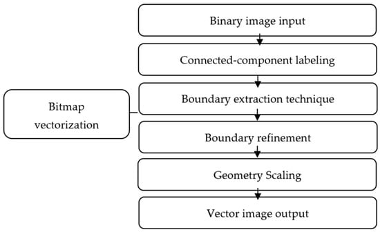
The transformation from a binary image to a vector image can be achieved using the following method. Figure 6 illustrates four steps, including connected-component labeling, the boundary extraction technique, boundary refinement, and geometry scaling.

In the connected-component labeling implementation, a digital image’s microstructure is stored as discrete pixels and grouped by a procedure. A binary image of n × m pixels is represented by $f(i,j)$ in the Cartesian coordinate system [37]:

$$f\left(i,j\right)=\left[\begin{array}{ccc}f\left(\mathrm{1,1}\right)& f\left(\mathrm{1,2}\right)& \begin{array}{cc}\cdots & f(1,m)\end{array}\\ f\left(\mathrm{2,1}\right)& f\left(\mathrm{2,2}\right)& \begin{array}{cc}\cdots & f(2,m)\end{array}\\ \begin{array}{c}⋮\\ f(n,1)\end{array}& \begin{array}{c}⋮\\ f(n,2)\end{array}& \begin{array}{c}\begin{array}{cc}& ⋮\end{array}\\ \begin{array}{cc}\cdots & f(n,m)\end{array}\end{array}\end{array}\right],i=\mathrm{1,2},\dots ,n,j=\mathrm{1,2},\dots ,m$$

(10)

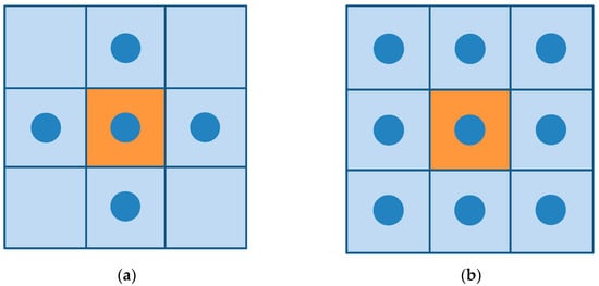
To obtain the microstructure’s geometry, such as pores or gravel, each pixel’s group is determined. A fast two-pass method algorithm segments the geometry into regions. A zero matrix of size f, a label variable l, and a label set variable li are initialized. The neighborhood Ω is shown in Figure 7, and a 4-neighbor domain is utilized. The first pass labels each pixel and its domain. A loop constructs domains with the same label.

To implement the boundary extraction technique, we utilized a method proposed for extracting the microstructure boundary from CT or NMR images [38]. The method labels the connected pixels using a region-growing algorithm, then divides each pixel into four edges, storing them in a list. Subsequently, the algorithm removes edges that appear twice in the list and connects the remaining edges to form a closed curve.

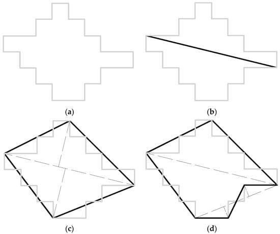
After determining the edges of the microstructure, in the boundary refinement step, microstructure edges are connected into a closed polyline using the Douglas–Peucker smooth algorithm (see Figure 8a). This polyline is jagged and has too many points, which are undesirable for numerical modeling. To smooth and reduce the number of points, we employed a boundary refinement algorithm described in Algorithm 1 [39]. This algorithm divides the vertices into two sections using the longest line (see Figure 8b). Subsequently, it calculates the line equation and the maximum distance from a vertex to the line as follows:

$$d=\left|\frac{\mathrm{A}{x}_0+B{y}_0+C}{\sqrt{A^2+B^2}}\right|$$

(11)

where $Ax+By+C=0$ is the line equation and ($x_0$, $y_0$) is the vertex coordinates. It repeats this for each section until the maximum distance is below a threshold (see Figure 8c). Finally, it obtains the refined boundary by connecting the edges (see Figure 8d).

Algorithm 1 Boundary refinement using Douglas–Peucker algorithm [39]

1: Set dt as the threshold distance, dp as perpendicular distance; 2: Find a separation line lm with the maximum length; 3: Separate El into two polylines as El(1) and El(2) with the line lm; 4: while dp >= dm; 5:  for i = 1 to length(El) do 6:     Calculate maximum dp to lm for the part BE(i) using Equation (2); 7:     if dp > dm, then 8:        Separate El(i) into two polylines El(1) and El(2); 9:        Replace El(i) with El (1) and El(2); 10:        Update the separation line; 11:     end; 12:  endfor; 13: end; 14: Set Bp as refined boundary; 15: for I = 1 to length(El) do 16:  Set the head and tail vertex as vh and vt; 17:  if i = 1 do 18:     Bp(1) = vh,Bp(2) = vt; 19:  else 20:     Bp(i + 1) = vt; 21:  endif; 22: endfor; 23: Return Bp.

The microstructure geometry in digital images is measured in pixels rather than physical distance (mm or μm). We employed a geometry scaling procedure to convert the geometry to the real size. Typically, the digital image has a proportional scale indicating the resolution. The real distance of a pixel can be estimated based on this information.

2.2.2. DEM Model Generation

The procedures in Section 2.2.1 transform a digital image into a vector graph consisting of numerous polygons. For heterogeneous materials with pores or aggregates, computing geometric statistics for the microstructure is crucial [40]. Three parameters, namely, the area, minimum bounding rectangle (MBR), and size and direction, are analyzed in the program.

• The area of a polygon with n vertices and coordinates ($x_k$, $y_k$) for the kth vertex can be calculated as follows:

  $$S=\left|\frac{1}{2}{\sum }_{k=1}^n\left(x_k{y}_{k+1}-x_{k+1}{y}_k\right)\right|.$$

  (12)
  By looping over all the polygons, we can obtain the statistical information of the area.
• MBR is a rectangle that encloses all the points in a given set of points and has the smallest area of all the enclosing rectangles. It is frequently used as an indicator of geographic features [41]. For each boundary polygon, a convex hull is computed. For each edge in the hull, the hull is rotated to obtain a possible rectangle. This process is performed for all the edges, and the smallest rectangle is selected. It is then rotated back to obtain the MBR.
• The particle size and direction are computed from the MBR of each particle. The short and long axes of the MBR correspond to the width and length of the particle, respectively. The width can serve as an approximation of the particle radius for composite materials. The direction is defined as the angle between the long axis and the horizontal line.

Statistical geometric information is crucial for creating high-quality numerical models. This information can be represented using vector graphics and converted to a drawing exchange format (DXF) file format. The conversion process maps the geometric shapes and paths from the source vector format to the corresponding entities in the DXF file.

3. Results and Discussion

3.1. Performance of the Instance Segmentation

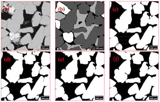
The size distribution of the Xiyu conglomerate was analyzed by segmenting the CT images. After iterative adjustments, the best algorithms were selected based on the validation results from UNet, HRNet, SegFormer, and the modified SegFormer. As depicted in Figure 9, the improved SegFormer generates binary and grayscale segmented images.

Three metrics, namely, intersection over union (IoU), dice coefficient, and F1 score, are employed to evaluate the predictive performance of different models. The intersection over union (IoU) measures the extent of overlap between the predicted positive samples and the actual positive samples.

$$IoU=\left(TP\right)/(TP+FP+FN)$$

(13)

In this context, TP represents the true positive count, FP represents the false positive count, and FN represents the false negative count. The IoU ranges from 0 to 1, with higher values indicating a greater overlap between the predicted results and the actual labels. An IoU of 1 indicates a perfect match between the predicted results and the actual labels.

The dice coefficient measures the similarity between the predicted positive samples and the actual positive samples, similar to IoU. The dice coefficient is more robust in handling segmentation tasks with class imbalance.

$$\mathrm{D}\mathrm{i}\mathrm{c}\mathrm{e}=(2\times \mathrm{T}\mathrm{P})/(2\times \mathrm{T}\mathrm{P}+\mathrm{F}\mathrm{P}+\mathrm{F}\mathrm{N})$$

(14)

The F1 score combines the precision and recall of a model.

$$\mathrm{F}1=2\times (\mathrm{Precision}\times \mathrm{Recall})/(\mathrm{Precision}+\mathrm{Recall})$$

(15)

Precision is the ratio of true positive predictions to all the positive predictions, while recall is the ratio of true positive predictions to all the actual positive samples.

The evaluation results of the three metrics for the four methods are presented in

Table 1. Segmentation accuracy of the four methods.

Algorithm/Metric	Label	IoU(%)	Dice(%)	F1(%)
UNet	gravel	81.78	89.97	89.97
	pore	56.87	72.51	72.51
	matrix	45.51	62.56	62.56
HRNet	gravel	82.47	90.39	90.39
	pore	62.3	76.77	76.77
	matrix	55.98	71.78	71.78
SegFormer	gravel	83.67	91.11	91.11
	pore	72.98	84.38	84.38
	matrix	59.2	74.37	74.37
ModSegFormer	gravel	86.24	92.61	92.61
	pore	77.81	87.52	87.52
	matrix	67.99	80.94	80.94

. It is evident that the SegFormer model outperforms UNet and HRNet in terms of accuracy by a significant margin. Additionally, HRNet exhibits slightly better accuracy than UNet. UNet performs exceptionally well in low-resolution images or small-sample segmentation tasks. However, when it comes to high-resolution CT image instance segmentation tasks, the decoder of UNet may not effectively handle long-range dependencies within high-resolution images. For certain instance segmentation tasks, instances may exhibit extensive feature connections, and the local feature propagation of UNet may be insufficient to capture such global dependencies. Moreover, in terms of multi-scale processing, the images may contain subtle structures and regions at different scales. HRNet is capable of handling these subtle differences without sacrificing resolution. In comparison, UNet primarily relies on the encoder–decoder architecture for information propagation and lacks the advantage of HRNet’s multi-branch approach for handling multi-scale information.

The SegFormer model demonstrated significant improvements in all the evaluation metrics compared to HRNet, particularly in accurately identifying pores. The SegFormer model incorporates a hierarchical Transformer encoder, efficiently handling multi-scale information. This is crucial for high-resolution CT image instance segmentation tasks, where images may contain details and structures at different scales. By effectively capturing these subtle differences, SegFormer enhances the accuracy of instance segmentation.

Through progressively integrating different features, the improved SegFormer model pays more attention to the distinctions between features at different scales, further enhancing segmentation accuracy, especially in recognizing matrices. The dice coefficient improved by 6.57, and the IoU improved by 8.79. The improved recognition results of SegFormer are displayed in Figure 10.

3.2. Model and Parameters

3.2.1. Numerical Simulation Model Generation

To study the mechanical properties of the Xiyu conglomerate, a numerical model was generated based on the porosity statistics and real CT reconstruction images in the previous section. The size of the model was the same as the actual size of the sample. To generate an accurate numerical simulation model, the first step is to import the previously generated DXF file into PFC. Next, according to the geometry, different properties of particles are filled into the model. Finally, the model is servoed. The specific steps to generate the model are as follows:

• Based on the porosity statistics in the previous section, we set the porosity to 0.2 and set the maximum-to-minimum particle size ratio Rmax/Rmin to 1.66. The file containing the coordinate points of the polygons generated earlier was imported into the PFC. The balls were automatically filled by approximating the medial surface of the geometry outlines.
• To simulate the different properties of various parts of the Xiyu conglomerate, we classified the contacts of the Xiyu conglomerate model into three categories. By judging the group to which the two ends of the contact belong, it can be divided into gravel contacts, matrix contacts, and gravel–matrix contacts.

The generated model is then subjected to servo control to achieve an ideal state of contact between the particle systems as quickly as possible, and a loading analysis is performed based on this state. This process is essential for using the discrete element method for mechanical analysis. For biaxial compression tests on the Xiyu conglomerate, the loading plates around the rock sample need to be adjusted to complete the servo control and stabilize its internal structure. This can be done by adjusting the servo speed in horizontal and vertical directions continuously. Meanwhile, the number of contacts between the particles and boundary walls is counted, and the servo parameter G for the next time step is calculated. The wall normal velocity $u_n^w$ is obtained again, and servo control for the next time step is started. This cycle is repeated until the average contact stress on all the boundary walls reaches the specified requirements. Assuming that $N_c$ is the number of particles in contact with the boundaries, $k_n$ is the average contact stiffness, ${\delta }_t$ is the time step length, $A$ is the wall area, $\alpha$ is the stress release factor, and ${\sigma }^{measured}$ and ${\sigma }^{required}$ are the measured stress and target stress on the loading plates, respectively. The servo adjustment coefficient and loading speed can be expressed, respectively, as follows:

$$G=\frac{\alpha A}{k_n{N}_c{\delta }_t}$$

(16)

$$u_n^w=G\ast abs({\sigma }^{measured}-{\sigma }^{required})$$

(17)

3.2.2. Parameter Calibration

In this study, a linear parallel bond model was used to characterize the macroscopic mechanical properties of the Xiyu conglomerate. The parallel-bond component acts in parallel with the linear component and establishes an elastic interaction between the pieces. The existence of a parallel bond does not preclude the possibility of slipping. Parallel bonds can transmit both force and moment between the pieces [19,42,43]. This model can provide two different interfaces of distinct mechanical behavior by simulating a finite-sized piece of cement-like material deposited between the two contacting pieces [44,45]. Due to the above-mentioned properties, this model can be applied to simulate the Xiyu conglomerate.

The discrete element numerical simulation of particles requires the input of micro-parameters that characterize the material properties. A common method for determining the micro-parameters for the discrete element simulation is based on the macro-mechanical parameters of the material and using numerical tests to calibrate the micro-parameters of the material [46].

Several parameters were calibrated in this study: the effective modulus ($E^{*}$) and parallel bond effective modulus (${\overline{E}}^{*}$) are the effective moduli for both the frictional interface and bonded interface, respectively, and they are roughly equal. The k ratio ($K^{*}$) and parallel bond k ratio (${\overline{K}}^{*}$) are the ratios between the normal and shear stiffness for each interface, respectively. The parallel bond tensile strength (${\overline{\sigma }}_c$) and parallel bond cohesion $\overline{c}$ are the micro-mechanical parameters that allow the bonded surface to withstand tensile and shear forces, respectively. The friction angle ($\overline{\phi }$) is analogous to the internal friction angle in the macro-mechanical parameters. The friction coefficient (μ) is the ratio between normal force and friction force. The micro-parameters of the Xiyu conglomerate are presented in

Table 2. Micro-mechanical DEM parameters of different parts of Xiyu conglomerate.

Contact Parameters	Composition
	Gravel	Matrix	Gravel–Matrix Interface
Effective modulus $E^{*}$ (Pa)	$5\times {10}^8$	$2.25\times {10}^8$	$4.5\times {10}^7$
K ratio $K^{*}$ (0–1)	1.25	1.25	1.25
Parallel bond effective modulus ${\overline{E}}^{*}$ (Pa)	$5\times {10}^8$	$2.25\times {10}^8$	$4.5\times {10}^7$
Parallel bond k ratio ${\overline{K}}^{*}$ (0–1)	1.25	1.25	1.25
Parallel bond tensile strength ${\overline{\sigma }}_c$ (Pa)	$4.5\times {10}^5$	$2.025\times {10}^5$	$4.05\times {10}^4$
Friction angle $\overline{\phi }$ (°)	45.0	40.0	40.0
Friction coefficient μ (0–1)	0.577	0.577	0.577
Parallel bond cohesion $\overline{c}$ (Pa)	$5\times {10}^5$	$2.25\times {10}^5$	$4.5\times {10}^4$

, where the corresponding mechanical parameter ratio of the matrix to the gravel is 0.45 and the gravel–matrix interface to the matrix is 0.2.

3.3. Destruction Process and Mechanical Characteristics

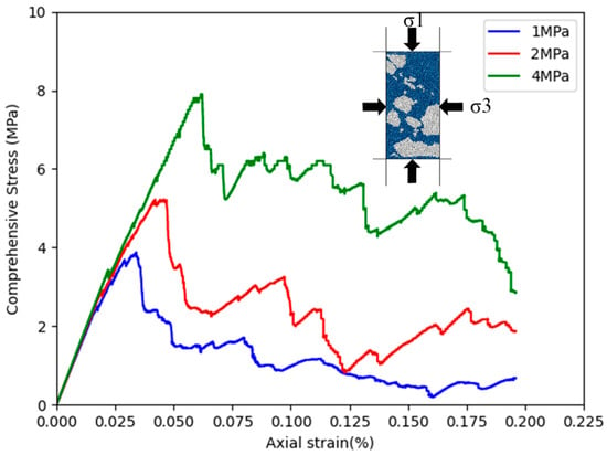
The internal friction angle and cohesion of rock are important indicators for evaluating the mechanical strength of the Xiyu conglomerate; therefore, based on the results of the parameter calibration, a biaxial compression test was conducted in this study on a Xiyu conglomerate model simulating a porosity of 20%. The lateral pressure plate applied a constant stress ${\sigma }_3$ to the rock sample, and the loading cover plate was set at a certain speed, which was equivalent to applying ${\sigma }_3+∆\sigma ={\sigma }_1$ to the rock sample. The confining pressures of the test were 1 MPa, 2 MPa, and 4 MPa, respectively.

3.3.1. Destruction Phase

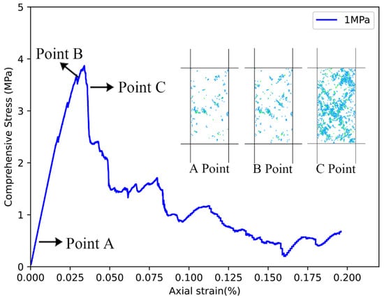
During the pre-peak phase (point A), the stress–strain curve forms an approximately straight line, signifying the model’s presence in the elastic phase. The formation of cracks is relatively limited, and those that do appear tend to align with the direction of maximum compression. These cracks are distributed across the specimen and appear to be non-interacting. A non-linear curve (point B) emerges as the strain increases before reaching the peak, signifying the model’s partial entry into the plastic phase with rapidly developing cracks. One or more macroscopic failure planes develop, cutting across the specimen. As the stress–strain curve transitions into the post-peak phase (point C), cracks continue evolving and join to form through cracks, leading to a rapid drop in the compressive stress and damage to the model. Figure 11 presents the resultant stress–strain curve, along with the entire crack development process across different stages.

3.3.2. Comparison of Mechanical Parameters

To comprehensively investigate and validate the mechanical properties of the Xiyu conglomerate, biaxial tests were conducted on samples subjected to varying confining pressures. Subsequently, the Mohr–Coulomb criterion was applied:

$$\tau \ge {\tau }_f=c+\sigma tan\phi$$

(18)

where $\tau$ is the shear stress on any section of the rock, ${\tau }_f$ is the critical shear stress at the onset of failure, c is the rock cohesion, and φ is the rock internal friction angle. The major and minor principal stresses ${\sigma }_1$ and ${\sigma }_3$ were obtained by monitoring the stress on the loading plates. Because the applied confining pressure was less than 10 MPa, the rock envelope line could be simplified as a straight line [47]. The internal friction angle of the rock sample was calculated to be 34.70°, and the rock cohesion was 0.64 MPa. The resultant stress–strain curves obtained through biaxial compression tests at different confinements are shown in Figure 12.

Fan [48] conducted a shear test on the Wuyi Reservoir in Xinjiang, from which the shear strength used in this paper was derived. The experiment determined that the natural internal friction angle of the Xiyu conglomerate is 39.0°, and the rock cohesion is 0.56 MPa. The comparison between the numerical experiment and the physical experiment is shown in

Table 3. Comparative analysis of parameters from numerical simulation and physical experiments.

Parameter	Physical Experiment	Numerical Experiment	Absolute Error	Relative Error/%
c	0.56 MPa	0.64 MPa	0.08 MPa	14.29
φ	39.0°	34.70°	4.3°	11.29

. The results show that the numerical experiment results are 14.29% higher than the laboratory results in cohesion and 11.29% lower in the internal friction angle φ.

4. Conclusions

Based on the CT images of the Xiyu conglomerate, we used various image processing techniques to conduct biaxial compression tests on the high-precision numerical model using the discrete element method. By analyzing the experimental data and the complete data processing workflow, we obtained the following conclusions:

• Based on the CT scan images, we proposed an improved SegFormer segmentation algorithm, which achieved high-accuracy instance segmentation by training the network after manually annotating the pores, matrix, and gravel. The performance of our method was compared with different algorithms under various evaluation methods, and the results show that our method was more accurate than the original one.
• The rock cohesion c of the Xiyu conglomerate is about 0.64 MPa, and the rock internal friction angle φ is about 34.70°. It has complex mechanical properties, manifested by various failure modes. The factors affecting the failure modes include the loading speed of the sample, the composition and distribution of the heterogeneous material, etc.

This study helps us to understand the causes and influencing factors of the anisotropy of the Xiyu conglomerate from the microstructure perspective and provides a micro-observation basis for establishing an anisotropic mechanical model of the Xiyu conglomerate. At the same time, the segmentation algorithm based on deep learning showed its power in this study, which will help us to obtain relevant information of rocks more conveniently in our future work.

References

- Chen, J.; Yin, J.; Qu, G.; Zhang, K. Timing, lower boundary, genesis, and defrormation of xiyu formation around the western margins of the tarim basin. Seismol. Geol. 2000, 22, 104–116. [Google Scholar]
- Li, B.; Wu, D.; Pang, L.; Lü, H.; Zheng, X.; Li, Y. Stratigraphic attribute and origin of the Xiyu conglomerates in NW China:progress and prospect. J. Earth Environ. 2019, 10, 427–440. [Google Scholar]
- Tian, W.; Chen, J.; Wu, B. Experimental study on material composition of Xiyu Formation calcareous cementitious conglomerate. Water Resour. Hydropower Eng. 2018, 49, 185–193. [Google Scholar]
- Fan, L.; Zhang, Y.-h.; Chen, C.; Wang, F.-x. Experimental research on resistance characteristics of surrounding rock of diversion tunnel in weak-cemented Xiyu conglomerate. Rock Soil Mech. 2019, 40, 2982–2988. [Google Scholar]
- Zhang, Q.; Zheng, Y.; Jia, C.; Sun, P.; Li, W. Investigation of the stability and failure mechanism of slopes in Xiyu conglomerate due to toe erosion. Bull. Eng. Geol. Environ. 2023, 82, 206. [Google Scholar] [CrossRef]
- Qin, X. Simulation study on damage mechanism of soft rock softening at the foot of Xiyu conglomerate high slopes. China Water Transp. 2019, 19, 258–259. [Google Scholar]
- Wang, Z.; Yuan, H.; Wang, D.; Zhang, Q. Back analysis of elastic resistance coefficient of tunnel surrounding rocks with measured displacement. J. Eng. Geol. 2013, 21, 143–148. [Google Scholar]
- Li, K.; Wang, Y.; Li, S.; Lin, X.; Sun, P.; Li, W. Study on failure mechanism of toe erosion of high Xiyu conglomerate slope. Water Resour. Hydropower Eng. 2017, 48, 184–190. (In Chinese) [Google Scholar]
- Meng, Q.; Wang, H.; Cai, M.; Xu, W.; Zhuang, X.; Rabczuk, T. Three-dimensional mesoscale computational modeling of soil-rock mixtures with concave particles. Eng. Geol. 2020, 277, 105802. [Google Scholar] [CrossRef]
- Yang, X. User Defined Heterogeneous Model Reconstruction and Internal Structure of Asphalt Concrete. Ph.D. Thesis, Michigan Technological University, Houghton, MI, USA, 2015. [Google Scholar]
- Abdulqader, A.; Rizos, D.C. Advantages of using digital image correlation techniques in uniaxial compression tests. Results Eng. 2020, 6, 100109. [Google Scholar] [CrossRef]
- Woodman, J.; Ougier-Simonin, A.; Stavrou, A.; Vazaios, I.; Murphy, W.; Thomas, M.E.; Reeves, H.J. Laboratory Experiments and Grain Based Discrete Element Numerical Simulations Investigating the Thermo-Mechanical Behaviour of Sandstone. Geotech. Geol. Eng. 2021, 39, 4795–4815. [Google Scholar] [CrossRef]
- Yu, Q.; Dai, Z.; Zhang, Z.; Soltanian, M.R.; Yin, S. Estimation of Sandstone Permeability with SEM Images Based on Fractal Theory. Transp. Porous Media 2019, 126, 701–712. [Google Scholar] [CrossRef]
- Qian, H.; Li, Y.; Yang, J.; Xie, L.; Tan, K.H. Segmentation and analysis of cement particles in cement paste with deep learning. Cem. Concr. Compos. 2023, 136, 104819. [Google Scholar] [CrossRef]
- Shi, C.; Yang, W.; Yang, J.; Chen, X. Calibration of micro-scaled mechanical parameters of granite based on a bonded-particle model with 2D particle flow code. Granul. Matter 2019, 21, 38. [Google Scholar] [CrossRef]
- Greco, O.D.; Ferrero, A.M.; Oggeri, C. Experimental and Analytical Interpretation of the Behaviour of Laboratory Tests on Composite Specimens. Int. J. Rock Mech. Min. Sci. Geomech. Abstr. 1993, 30, 1539–1543. [Google Scholar] [CrossRef]
- Jing, L. A review of techniques, advances and outstanding issues in numerical modelling for rock mechanics and rock engineering. Int. J. Rock Mech. Min. Sci. 2003, 40, 283–353. [Google Scholar] [CrossRef]
- Cundall, P.A.; Strack, O.D.L. A discrete numerical model for granular assemblies. Géotechnique 1980, 30, 331–336. [Google Scholar] [CrossRef]
- Itasca. PFC 5.0 Documentation, 5.0; Itasca Consulting Group: Minneapolis, MN, USA, 2016. [Google Scholar]
- Board, M. UDEC (Universal Distinct Element Code) Version ICG1. 5; Nuclear Regulatory Commission: Washington, DC, USA, 1989. [Google Scholar]
- Govender, N.; Wilke, D.N.; Pizette, P.; Abriak, N.E. A study of shape non-uniformity and poly-dispersity in hopper discharge of spherical and polyhedral particle systems using the Blaze-DEM GPU code. Appl. Math. Comput. 2018, 319, 318–336. [Google Scholar] [CrossRef]
- Lee, S.J.; Hashash, Y.M.A.; Nezami, E.G. Simulation of triaxial compression tests with polyhedral discrete elements. Comput. Geotech. 2012, 43, 92–100. [Google Scholar] [CrossRef]
- Shi, C.; Zhang, Q.; Wang, S. Numerical Simulation Techniques and Applications for Particle Flow (PFC5.0), 1st ed.; China Construction Industry Press: Nanjing, China, 2018; p. 449. [Google Scholar]
- Radjai, F.; Cheng, H.; Shuku, T.; Thoeni, K.; Yamamoto, H.; Nezamabadi, S.; Luding, S.; Delenne, J.Y. Calibration of micromechanical parameters for DEM simulations by using the particle filter. EPJ Web Conf. 2017, 140, 12011. [Google Scholar]
- Liu, G.-Y.; Xu, W.-J.; Zhou, Q.; Zhang, X.-L. Contact Overlap Calculation Algorithms and Benchmarks Based on Blocky Discrete-Element Method. Int. J. Geomech. 2022, 22. [Google Scholar] [CrossRef]
- Russell, B.C.; Torralba, A.; Murphy, K.P.; Freeman, W.T. LabelMe: A database and web-based tool for image annotation. Int. J. Comput. Vis. 2008, 77, 157–173. [Google Scholar] [CrossRef]
- Lin, T.-Y.; Maire, M.; Belongie, S.; Hays, J.; Perona, P.; Ramanan, D.; Dollár, P.; Zitnick, C.L. Microsoft coco: Common Objects in Context. In Computer Vision–ECCV 2014: 13th European Conference, Zurich, Switzerland, 6–12 September 2014, Proceedings, Part V 13, 2014; Springer: Berlin/Heidelberg, Germany, 2014; pp. 740–755. [Google Scholar]
- Cordts, M.; Omran, M.; Ramos, S.; Rehfeld, T.; Enzweiler, M.; Benenson, R.; Franke, U.; Roth, S.; Schiele, B. The Cityscapes Dataset for Semantic Urban Scene Understanding. In Proceedings of the IEEE Conference on Computer Vision and Pattern Recognition, Las Vegas, NV, USA, 27–30 June 2016; IEEE: Las Vegas, NV, USA, 2016; pp. 3213–3223. [Google Scholar]
- Wang, Z.; Wang, Q.; Yang, Y.; Liu, N.; Chen, Y.; Gao, J. Seismic Facies Segmentation via a Segformer-Based Specific Encoder–Decoder–Hypercolumns Scheme. IEEE Trans. Geosci. Remote Sens. 2023, 61, 1–11. [Google Scholar] [CrossRef]
- Li, M.; Rui, J.; Yang, S.; Liu, Z.; Ren, L.; Ma, L.; Li, Q.; Su, X.; Zuo, X. Method of Building Detection in Optical Remote Sensing Images Based on SegFormer. Sensors 2023, 23, 1258. [Google Scholar] [CrossRef] [PubMed]
- Xie, E.; Wang, W.; Yu, Z.; Anandkumar, A.; Alvarez, J.M.; Luo, P. SegFormer: Simple and efficient design for semantic segmentation with transformers. Adv. Neural Inf. Process. Syst. 2021, 34, 12077–12090. [Google Scholar]
- Ronneberger, O.; Fischer, P.; Brox, T. U-net: Convolutional Networks for Biomedical Image Segmentation. In Medical Image Computing and Computer-Assisted Intervention–MICCAI 2015: 18th International Conference, Munich, Germany, 5–9 October 2015, Proceedings, Part III 18; Springer: Berlin/Heidelberg, Germany, 2015; pp. 234–241. [Google Scholar]
- Sun, K.; Zhao, Y.; Jiang, B.; Cheng, T.; Xiao, B.; Liu, D.; Mu, Y.; Wang, X.; Liu, W.; Wang, J. High-resolution representations for labeling pixels and regions. arXiv 2019, arXiv:1904.04514. [Google Scholar]
- Wang, J.; Zhang, J.-H.; Zhang, J.-L.; Lu, F.-M.; Meng, R.-G.; Wang, Z. Research on fault recognition method combining 3D Res-UNet and knowledge distillation. Appl. Geophys. 2021, 18, 199–212. [Google Scholar] [CrossRef]
- Wang, J.; Sun, K.; Cheng, T.; Jiang, B.; Deng, C.; Zhao, Y.; Liu, D.; Mu, Y.; Tan, M.; Wang, X. Deep High-Resolution Representation Learning for Visual Recognition. IEEE Trans. Pattern Anal. Mach. Intell. 2021, 43, 3349–3364. [Google Scholar] [CrossRef]
- Meng, Q.-X.; Xu, W.-Y.; Wang, H.-L.; Zhuang, X.-Y.; Xie, W.-C.; Rabczuk, T. DigiSim—An Open Source Software Package for Heterogeneous Material Modeling Based on Digital Image Processing. Adv. Eng. Softw. 2020, 148, 102836. [Google Scholar] [CrossRef]
- Gonzalez, R.C.; Woods, R.E.; Masters, B.R. Digital Image Processing, 3rd ed.; Prentice Hall: Upper Saddle River, NJ, USA, 2009; Volume 14. [Google Scholar]
- Yan, L.; Meng, Q.X.; Xu, W.Y.; Wang, H.L.; Zhang, Q.; Zhang, J.C.; Wang, R.B. A numerical method for analyzing the permeability of heterogeneous geomaterials based on digital image processing. J. Zhejiang Univ. Sci. A 2017, 18, 124–137. [Google Scholar] [CrossRef]
- Chen, S.; Yue, Z.Q.; Tham, L.G. Digital Image Based Approach for Three-Dimensional Mechanical Analysis of Heterogeneous Rocks. Rock Mech. Rock Eng. 2007, 40, 145. [Google Scholar] [CrossRef]
- Morin, Z.Q.Y. Isabelle, Digital image processing for aggregate orientation in asphalt concrete mixtures. Can. J. Civ. Eng. 1996, 23, 480–489. [Google Scholar]
- Sleit, A.; Salah, I.; Jabay, R. Approximating Images Using Minimum Bounding Rectangles. In Proceedings of the 2008 First International Conference on the Applications of Digital Information and Web Technologies (ICADIWT), Ostrava, Czech Republic, 4–6 August 2008. [Google Scholar]
- Potyondy, D.O.; Cundall, P.A. A bonded-particle model for rock. Int. J. Rock Mech. Min. Sci. 2004, 41, 1329–1364. [Google Scholar] [CrossRef]
- Song, H.; Meng, Q.; Guo, N.; Chen, X.; Xu, W.; Cao, Y. Modeling of Fracture Behavior of Four-Phase Concrete using a DEM-enhanced Structure Generation. Int. J. Multiscale Comput. Eng. 2024; in press. [Google Scholar]
- Ding, Y.; Zhang, Q.; Zhao, S.; Chu, W.; Meng, Q. An improved DEM-based mesoscale modeling of bimrocks with high-volume fraction. Comput. Geotech. 2023, 157, 105351. [Google Scholar] [CrossRef]
- Meng, Q.; Xue, H.; Song, H.; Zhuang, X.; Rabczuk, T. Rigid-block DEM modeling of mesoscale fracture behavior of concrete with random aggregates. J. Eng. Mech. 2023, 149, 04022114. [Google Scholar] [CrossRef]
- Wang, Y.; Sun, P.; Li, W.; Zhang, Q. Failure mechanism and stability analysis method of the Xiyu conglomerate slope. J. Tsinghua Univ. Sci. Technol. 2021, 61, 863–872. [Google Scholar]
- Xu, Z. Rock Mechanics, 3rd ed.; China Water Conservancy and Hydropower Press: Nanjing, China, 2005; pp. 48–49. [Google Scholar]
- Fan, H. Test Research on Structure Characteristics and Mechanical Characteristics of Xiyu Conglomerate; Beijing Jiaotong University: Beijing, China, 2016. [Google Scholar]
Disclaimer/Publisher’s Note: The statements, opinions and data contained in all publications are solely those of the individual author(s) and contributor(s) and not of MDPI and/or the editor(s). MDPI and/or the editor(s) disclaim responsibility for any injury to people or property resulting from any ideas, methods, instructions or products referred to in the content. |
© 2023 by the authors. Licensee MDPI, Basel, Switzerland. This article is an open access article distributed under the terms and conditions of the Creative Commons Attribution (CC BY) license (https://creativecommons.org/licenses/by/4.0/).