Article

An Improved Data-Driven Integral Sliding-Mode Control and Its Automation Application

1
School of Mechanical and Electrical Engineering, Quzhou College of Technology, Quzhou 324000, China
2
College of Communication Engineering, Jilin University, Changchun 130022, China
3
Quzhou Special Equipment Inspection Center, Quzhou 324000, China
*
Author to whom correspondence should be addressed.
Appl. Sci. 2023, 13(24), 13094; https://doi.org/10.3390/app132413094
Submission received: 20 September 2023 / Revised: 2 December 2023 / Accepted: 4 December 2023 / Published: 8 December 2023

Abstract

:
Circulating fluidized bed (CFB) boilers are widely used in industrial production due to their high combustion efficiency, low pollutant emissions and wide load-adjustment range. However, the water-level-control system of a CFB boiler exhibits time-varying behavior and nonlinearity, which affect the control performance of the industrial system. This paper proposes a novel data-driven adaptive integral sliding-mode control (ISMC) method for the CFB control system with external disturbances. Firstly, the scheme designs a discrete ISMC law based on the full-format dynamic linearization (FFDL) data model, which is equivalent to a nonlinear system. Furthermore, a new reaching law is proposed to quickly drive the system state onto the sliding-mode surface. The improved ISMC control scheme only utilizes the input–output data during the design process and does not require model information. After theoretically verifying the stability of the method proposed in this paper, it is further applied in MIMO systems. Finally, the control and practical effects of this method are evaluated by using the DHX25-1.25 CFB boiler installed in the special-equipment testing center. The experimental results show that, compared with the traditional sliding-mode control (SMC) and model-free adaptive-control (MFAC) methods, the improved control method can quickly track the given signal and exhibit resistance to noise interference. Furthermore, it can rapidly respond to changes in the working conditions of the CFB system.

1. Introduction

The water-level system of a CFB boiler is used to ensure the fluidity of the soft water circulation system in order to absorb the waste heat from the boiler’s flue gas. The design of its control scheme is of great significance for ensuring the operational safety and production efficiency of the system. Therefore, under the premise of ensuring safe production, further improving the balance of boiler water-level control has become a research hotspot. However, in the actual production process, the water-level-control system of CFB boilers may be affected by many external factors and exhibit characteristics such as time variance and nonlinear models [1,2]. These characteristics significantly impact the control performance of the system. Therefore, designing a high-performance method for controlling the boiler water level is very beneficial for further improving industrial efficiency and realizing green and energy-saving production.
In industrial production, the CFB boiler water-level-control system plays a crucial role, and many scholars have conducted in-depth research on this. The control methods designed can be roughly divided into model-based control methods and data-driven control methods. Among them, the model-based control method has a simple design process, and the system stability analysis is relatively simple. However, in practical situations, the CFB boiler system is affected by various uncertain factors, making it difficult to establish an accurate model of the system. Therefore, model-based control methods have inherent shortcomings [3,4]. Data-driven control methods are widely used in boiler water-level-control systems because they do not rely on a precise mathematical model and can only rely on system input and output data to achieve system control. Among them, the most typical data-driven control method is PID. Ref. [5] proposed an expert PID method that can still achieve stable control even when the boiler water level is greatly disturbed. Ref. [6] designed an incomplete differential PID to achieve precise control of the boiler-drum water level, thereby ensuring the energy-saving operation of the system. Ref. [7] considers the characteristics of nonlinearity, multivariability and large time delays in the CFB boiler system and uses the fuzzy PID method to control the system, effectively improving the operational efficiency of the system. Ref. [8] combines fuzzy theory to design a fuzzy-PID hybrid control method, which achieves intelligent control of the water level of the thermal boiler drum and effectively avoids the influence of external disturbances on water-level control. Ref. [9] proposes a control strategy that combines the DMC prediction algorithm with feedforward cascade control. DMC-PID feedforward cascade control is used to achieve stable control of the boiler water level and improve its dynamic and static characteristics. However, when using PID to realize the automated operation of the system, due to the fixed parameters of the controller, there are shortcomings that cannot realize the adaptive adjustment. Although the most widely used PID control does not require mathematical modeling, it is more suitable for linear systems and is not suitable for nonlinear, time-varying and strongly coupled systems. In addition, it does not have the ability to learn and adapt to changes in the system structure, so the control performance is poor, slow and prone to overshooting [10,11].
At the end of the 20th century, professor Hou proposed a model-free adaptive-control (MFAC) method. This method uses a data model equivalent to the controlled system to design the controller and introduces the concept of pseudopartial derivatives to realize the adaptive adjustment of the controller parameters, thus realizing the adaptive control of the controlled system [12]. Due to the excellent control performance of MFAC, this method has been widely used in many industrial fields. Ref. [13] applied MFAC theory to the heading control system of unmanned surface vessels, achieving precise heading control of the system under model disturbances and system delays. Ref. [14] designed a model-free adaptive fault-tolerant control method that considers issues such as subway speed and traction force constraints, as well as actuator failures, achieving precise control of the subway train. Ref. [15] utilized the MFAC method to realize automobile autopilot, which improved the accuracy, safety and comfort of automobile control. Ref. [16] introduced the MFAC into the self-resistant controller and designed a new type of self-resistant controller to realize the stable heading control of a ship. Ref. [17] designed a new data-driven model-free adaptive robust control law, which was applied the control algorithm to unmanned helicopters and achieved good attitude-control results. Ref. [18] utilized the principle of MFAC to achieve precise control and multiobjective stable control of a continuous robotic arm. In addition, MFAC has been widely used in rehabilitation robots [19], coal-mine belt conveyors [20], linear motors [21], chemical production [22] and other fields.
Due to the excellent control performance of MFAC, it has been widely used and developed in many industrial fields, and some scholars have introduced MFAC into the control of the CFB water level. Ref. [23] introduced an improved tracking differentiator on the basis of MFAC and designed a noise-resistant MFAC method, which realized the noise-resistant control of the CFB water level, but the control accuracy needs to be improved. Ref. [24] utilized the MFAC method to achieve water-level control in the boiler water circulation system. A mode search algorithm was used to optimize the MFAC parameters, which greatly improved the accuracy of the water-level control but did not consider the influence of external disturbances. Ref. [25] derived a new control law with an error rate by adding an error rate to the objective criterion function and fusing and weighting the error and error rate, and the new control method can not only quickly track a given signal but also has good resistance to noise interference. However, if the signal is time-varying, the tracking effect will be affected. Since MFAC relies on real-time sample data for adaptive adjustment, it is sensitive to environmental changes. If the environmental changes are too drastic or the sample data are inaccurate, the MFAC may not be able to adapt to the new environmental conditions in time, resulting in a degradation of the control performance [26].
To further improve the control accuracy and robustness of the CFB boiler control system, it must overcome the influence of large disturbances, multiple parameters and strong coupling in the CFB boiler control system and achieve precise control of the CFB boiler water level. This paper considers introducing the idea of the parameter adaptation of MFAC and combining it with the principle of SMC to design a new model-free adaptive ISMC method to further optimize the control effect of the system. The scheme is based on the FFDL data model in model-free adaptive control, and the discrete ISMC law is designed to realize the control of the system. Finally, the method is simulated and tested on a DHX25-1.25 CFB boiler, which is equipped in the special-equipment testing center. It is then compared with the traditional MFAC and SMC control methods. This proves that the improved control method can quickly track the given signals and has good resistance to noise interference.
The specific contributions of this paper are mainly in three aspects:
(1)
A new ISMC algorithm is proposed, which alleviates the chattering phenomenon of the system compared to the methods in [26,27]. The algorithm utilizes the improved sliding-mode surface and the convergence law to achieve more-efficient nonlinear control. At the same time, the algorithm also solves the problems of randomly selecting initial weights and excessive control parameters in traditional neural networks.
(2)
The FFDL data model used in this paper has the following advantages: High flexibility—the FFDL data model has high flexibility and can adapt to different types and structures of controlled systems. It can handle any amount and type of data sets, and the linearization length can be easily added, deleted or modified. Strong adaptability—The FFDL data model is very suitable for use in scenarios with frequent demand changes or unstable data structures. And, this data model does not require precise parameter information of the system and can handle systems with fast, unknown or unmeasurable parameter changes. It can also automatically learn and adjust control strategies to adapt to new changes.
(3)
Compared with most of the existing CFB control algorithms, the control scheme in this paper does not rely on the process model of the boiler water-level system and is a data-driven control scheme. The scheme can provide more accurate results, and by analyzing a large amount of real-time data, more accurate and reliable results and predictions can be obtained.
The aim of this study is to propose a novel model-free adaptive ISMC scheme to address the issues existing in the water-level-control system of circulating fluidized bed boilers. The proposed scheme equivalently linearizes the nonlinear system into an FFDL data model by using the dynamic linearization method. Then, a discrete-time double integral sliding-mode control law and a new reaching law are designed to improve the control-precision and disturbance-rejection performance. This study is practical and advanced, and it is of great significance for improving the performance of the water-level-control system in circulating fluidized bed boilers in industrial production. It provides useful references for the technological development and application in related fields.
Section 2 provides the flow of the traditional MFAC method. Section 3 proposes the ISMC method based on the FFDL data model and rigorously proves its stability. Section 4 shows the numerical and boiler water-level-system simulation experiments.
Lemma 1
([28]). Consider the following scalar dynamical system:
x ( i + 1 ) = x ( i ) c 1 sig α x ( i ) c 2 x ( i ) + l ( i )
If l ( i ) < R , then x ( i ) is bounded, and the following equation always holds:
x ( i ) 1 + α α 1 α α 1 1 α · max R c 1 1 α , c 1 1 c 2 1 1 α i i

2. Traditional Model-Free Adaptive Controller

2.1. Dynamic Linearization

Consider a class of discrete-time nonlinear systems that can be represented as follows:
I ( i + 1 ) = f I ( i ) , , I ( i n I ) , O ( i ) , , O ( i n O )
where O ( i ) and I ( i ) denote the input and output, respectively. n O and n I are the orders. f ( · ) is a nonlinear function.
Define L ( i ) as follows:
L ( i ) = [ Δ I ( i ) , , Δ I ( i L I + 1 ) , Δ O ( i ) , , Δ O ( i L O + 1 ) ] T
where L I and L O are the linearization length constants, also known as pseudo-orders.
Assumption 1
([29]). The partial derivatives of f ( · ) for all variables of the system exist.
Assumption 2
([29]). For any i 1 i 2 0 and L ( i 1 ) L ( i 2 ) , one has
I ( i 1 + 1 ) I ( i 2 + 1 ) p L ( i 1 ) L ( i 2 )
where p > 0 is a constant.
Theorem 1
([29]). For a time-varying system (1) satisfying Assumptions 1 and 2, when Δ L ( i ) 0 , then there must exist a parameter vector H ( i ) [29], which makes the following hold:
I ( i + 1 ) = I ( i ) + H T ( i ) Δ L ( i )
where the time-varying parameter vector is defined as H ( i ) = [ h 1 ( i ) , , h L I + L O ( i ) ] T .
Remark 1.
Theorem 1 has been proven [29]. Choosing different linearization length constants can result in different FFDL data models. The reasonable selection of the time-varying parameter vector and length constant can improve the accuracy of the data model in describing the system.

2.2. Traditional MFAC Design

Consider the following performance-metric function:
λ O ( i ) = O ( i ) O ( i 1 ) 2 + I d ( i + 1 ) I ( i + 1 ) 2
where I d is the desired output and > 0 is a weighting factor.
The control law is obtained by taking (7) to the first order partial differentiation of O ( i ) and making it zero as follows:
O ( i ) = O ( i 1 ) + ρ L I + 1 h L I + 1 ( i ) ( I d ( i + 1 ) I ( i ) ) + h L I + 1 ( i ) 2 h L y + 1 ( i ) k = 1 L I ρ k h k ( i ) Δ I ( i k + 1 ) + k = L I + 2 L I + L O ρ k h k ( i ) Δ O ( i L I k + 1 ) + h L I + 1 ( t ) 2
where ρ ( 0 , 1 ] is the step factor.
The following estimation function is utilized to accurately estimate the time-varying parameter vector H ( i ) :
J H ( i ) = Δ I ( i ) H T ( i ) Δ L ( i 1 ) 2 + μ H ( i ) H ^ ( i 1 ) 2
where μ > 0 is the weight factor.
The parameter estimation algorithm is given by the minimization of the parameter estimation criterion function (9):
H ^ ( i ) = H ^ ( i 1 ) + η Δ L ( i 1 ) Δ I ( i ) H ^ T ( i 1 ) Δ L ( i 1 ) μ + Δ L ( i 1 ) 2
where H ^ ( i ) is the estimated value of H ( i ) and η ( 0 , 2 ] is the step factor.
Design parameter reset algorithms to further enhance the system’s anti-interference ability:
H ^ ( i ) = H ^ ( 1 ) if H ^ ( i ) ε or Δ L ( i 1 ) 2 ε or sign h ^ L I + 1 ( i ) sign h ^ L I + 1 ( 1 )
The control scheme is obtained as follows:
Δ O ( i ) = ρ L I + 1 h ^ L I + 1 ( i ) ( I d ( i + 1 ) I ( i ) ) + h ^ L I + 1 ( i ) 2 h ^ L y + 1 ( i ) k = 1 L I ρ k h ^ k ( i ) Δ I ( i k + 1 ) + k = L I + 2 L I + L O ρ k h ^ k ( i ) Δ O ( i L I k + 1 ) + h ^ L I + 1 ( t ) 2 H ^ ( i ) = H ^ ( i 1 ) + η Δ L ( i 1 ) Δ I ( i ) H ^ T ( i 1 ) Δ L ( i 1 ) μ + Δ L ( i 1 ) 2 H ^ ( i ) = H ^ ( 1 ) if H ^ ( t ) ε or Δ L ( i 1 ) 2 ε or sign h ^ L I + 1 ( i ) sign h ^ L I + 1 ( 1 )
where the ρ ( 0 , 1 ] is the step factor.

3. Improved Model-Free Adaptive Sliding-Mode Controller

3.1. Integral Sliding-Mode Controller

Define the system output error as
e ( i ) = I ( i ) I d ( i )
Inspired by the algorithm in [27], consider designing the following sliding-mode function:
ν ( i ) = e ( i ) + c 1 E ( i 1 ) + c 2 F ( i 1 )
where 0 < c 1 < 1 , 0 < c 2 < 1 . The two integral error terms can be defined as follows:
E ( i ) = k = 0 i e ( k ) = E ( i 1 ) + e ( i )
F ( i ) = k = 0 i sig α e ( k ) = F ( i 1 ) + sig α e ( i )
Subsequently, the following reaching law is given:
Δ ν ( i + 1 ) = ν ( i + 1 ) ν ( i ) = 0
Combining (13), (14) and (17), it is not difficult to obtain
ν ( i ) = ν ( i + 1 ) = e ( i + 1 ) + c 1 E ( i ) + c 2 F ( i ) = I ( i + 1 ) I d ( i + 1 ) + c 1 E ( i ) + c 2 F ( i )
Substituting the data model (6) into (18), the following can be obtained:
ν ( i ) = I ( i ) + h ^ 1 ( i ) Δ I ( i ) + h ^ 2 ( i ) Δ O ( i ) I d ( i + 1 ) + c 1 E ( i ) + c 2 F ( i )
From (19), the equivalent control-law expression can be derived:
Δ O e q ( i ) = h ^ 2 1 ( i ) ν ( i ) c 1 E ( i ) c 2 F ( i ) + I d ( i + 1 ) I ( i ) h ^ 1 ( i ) Δ I ( i )
To improve the robustness of the system and alleviate the chattering phenomenon, the following switching law is introduced [26,27]:
Δ O s w ( i ) = h ^ 2 1 ( i ) β sgn ν ( i )
where 0 < β denotes the switching gain.
Based on the above analysis, the data-driven ISMC scheme can be obtained as follows:
Δ O ( i ) = Δ O e q ( i ) + Δ O s w ( i ) Δ O e q ( i ) = h ^ 2 1 ( i ) ν ( i ) c 1 E ( i ) c 2 F ( i ) + I d ( i + 1 ) I ( i ) h ^ 1 ( i ) Δ I ( i ) Δ O s w ( i ) = h ^ 2 1 ( i ) β sgn ν ( i ) ν ( i ) = e ( i ) + c 1 E ( i 1 ) + c 2 F ( i 1 ) E ( i ) = k = 0 i e ( k ) = E ( i 1 ) + e ( i ) F ( i ) = k = 0 i sig α e ( k ) = F ( i 1 ) + sig α e ( i )
Remark 2.
The following saturation function can be considered instead of the sign function:
sat σ = sgn σ ) , σ > X σ / X , σ < X
where X > 0 .
The control block diagram is shown in Figure 1.

3.2. Stability Analysis

Theorem 2.
For the system (3) with external perturbations, if the control scheme adopts (22), the controlled system satisfies the following properties:
(1)
H ^ ( i ) is bounded;
(2)
Under any initial conditions, the system can reach the quasisliding-mode state;
(3)
e ( i ) converges to the region E e , where
E e = e ( i ) 1 + r r 1 r r 1 1 r · max β c 1 1 r , c 1 1 c 2 1 1 r
Proof. 
H ^ ( i ) is bounded.
Subtracting H ( i ) from both sides of (10) simultaneously:
H ˜ ( i ) = H ˜ ( i 1 ) + H ( i 1 ) H ( i ) + β I ( i ) I ( i 1 ) Δ L T ( i 1 ) μ + Δ L ( i 1 ) 2 β H ˜ ( t 1 ) + H ( t 1 ) Δ H ¯ ( i 1 ) Δ L T ( i 1 ) μ + Δ L ( i 1 ) 2
Substituting the (6) into (25) yields
H ˜ ( i ) = H ˜ ( i 1 ) 1 β Δ L ( i 1 ) Δ L T ( i 1 ) μ + Δ L ( i 1 ) 2 + H ( i 1 ) H ( i )
Since H ( i ) is bounded, let its upper bound be H ( i ) x . Taking the norm on both sides of (26), we have
H ˜ ( i ) H ˜ ( i 1 ) 1 β Δ L ( i 1 ) Δ L T ( i 1 ) μ + Δ L ( i 1 ) 2 + 2 x
Square the first term of (27):
H ˜ ( i 1 ) 1 β Δ L ( i 1 ) Δ L T ( i 1 ) μ + Δ L ( i 1 ) 2 2 = H ˜ ( i 1 ) 2 + β Δ L ( i 1 ) 2 μ + Δ L ( i 1 ) 2 2 β H ˜ ( i 1 ) 2 Δ L ( i 1 ) 2 μ + Δ L ( i 1 ) 2
Since the step factor η ( 0 , 2 ] and μ > 0 , it is not difficult to obtain
β Δ L ( i 1 ) 2 μ + Δ L ( i 1 ) 2 < β Δ L ( i 1 ) 2 Δ L ( i 1 ) 2 < 2
Through (28) and (29), it can be inferred that
H ˜ ( i 1 ) 1 β Δ L ( i 1 ) Δ L T ( i 1 ) μ + Δ L ( i 1 ) 2 2 < H ˜ ( i 1 ) 2
From (30), there must exist a number 0 < M 1 < 1 :
H ˜ ( i 1 ) 1 β Δ L ( i 1 ) Δ L T ( i 1 ) μ + Δ L ( i 1 ) 2 = M 1 H ˜ ( i 1 )
Substituting (31) into (27) yields the following inequality:
H ˜ ( i ) M 1 H ˜ ( i 1 ) + 2 x M 1 M 1 H ˜ ( i 2 ) + 2 x + 2 x M 1 i 1 H ˜ ( 1 ) + 1 M 1 i 1 1 M 1 2 x
From (32), it follows that H ˜ ( i ) is bounded. Since H ( i ) is bounded, it follows that H ^ ( i ) is bounded. □
Proof. 
The system will reach quasisliding modes.
Substituting (6) into (13), the following can be obtained:
e ( t + 1 ) = y d y ( t + 1 ) = y d y ( t ) ϕ 1 Δ y ( t ) ϕ 2 Δ u ( t )
Substituting (22) into (33), the following can be obtained:
e ( i + 1 ) = ν ( i ) c 1 E ( i ) c 2 F ( i ) β sgn ν ( i )
Substituting (34) into (14), the following can be obtained:
ν ( i + 1 ) = ν ( i ) β sgn ν ( i )
From (35), it can be inferred that
ν ( i + 1 ) < ν ( i )
In summary, it can be seen that the system meets the conditions for the existence and arrival of sliding modes. Therefore, ν ( i ) monotonically decreases and reaches a quasisliding mode.
Proof. 
Substituting (14) into (34), the following can be obtained:
e ( i + 1 ) = ν ( i ) c 1 E ( i ) c 2 F ( i ) β sgn ν ( i ) = e ( i ) c 1 e ( i ) c 2 sig α e ( i ) β sgn ν ( i )
According to the Lemma 1 and (37), the convergence expression can be obtained:
e ( i ) 1 + r r 1 r r 1 1 r · max β c 2 1 r , c 2 1 c 1 1 1 r
From (38), the tracking error is bounded.
In summary, using the control scheme (22), the output of the system can successfully track the desired output. □

4. Simulation and Experiment

The first group is a typical numerical simulation experiment, using the FFDL-ISMC and the traditional sliding-mode control (FFDL-SMC) for comparison. The second group of experiments is performed to add perturbation signals and apply the FFDL-ISMC method to the control of the CFB water level. Traditional model-free adaptive-control (FFDL-MFAC), FFDL-SMC and model-free nonsingular high-order terminal sliding-mode-control (MFNHTSMC) methods were added to compare and analyze indicators such as the MSE, MAE, adjustment time, rise time, etc.

4.1. Experiment 1: Numerical Simulation

To increase the applicability of this paper’s method, it is extended to an MIMO system. The effectiveness of the proposed algorithm is verified through the simulation of a typical controlled object, and the FFDL-SMC and FFDL-ISMC algorithms are compared under time-varying signals. The first set of simulation objects is a three-input three-output system as follows:
I 1 ( i + 1 ) = 0.5 × d ( i ) + 1.5 × I 1 ( i ) + 0.12 × I 1 2 ( i 1 ) + 0.8 × O 1 ( i ) + 0.1 × O 2 ( i ) + 0.2 × O 3 ( i ) I 2 ( i + 1 ) = 0.5 × d ( i ) + 1.6 × I 2 ( i ) + 0.14 × I 2 2 ( i 1 ) + 0.1 × O 1 ( i ) + 0.8 × O 2 ( i ) + 0.2 × O 3 ( i ) I 3 ( i + 1 ) = 0.5 × d ( i ) + 1.6 × I 3 ( i ) + 0.15 × I 3 2 ( i 1 ) + 0.2 × O 1 ( i ) + 0.1 × O 2 ( i ) + 0.8 × O 3 ( i )
The desired output is set as follows:
I d = lins ( 0 , 50 , 100 ) × 5 , [ 0 , 100 ] lins ( 250 , 250 , 50 ) , [ 100 , 150 ] lins ( 250 , 290 , 50 ) , [ 150 , 200 ] lins ( 290 , 290 , 525 ) , [ 200 , 725 ] lins ( 290 , 0 , 275 ) , [ 725 , 1000 ]
where the lins ( k 1 , k 2 , x ) function is used to generate a vector of x-point rows between k 1 and k 2 , with the same span of neighboring data, and k 1 , k 2 and x are the start value, the end value and the number of elements, respectively.
The FFDL-ISMC and FFDL-SMC controller parameters are set to H ^ 1 ( 1 ) = H ^ 2 ( 1 ) = diag { 0.6 , 0.6 , 0.6 } , η = 0.75 , μ = 1 , β = 0.02 , θ = 0.2 , c 1 = 0.45 , c 2 = 25 , L I = 1 , L O = 1 , α = 0.5 .
Figure 2 shows the output curves of FFDL-ISMC and FFDL-SMC, and Figure 3 shows the output error curves. As can be seen from the enlarged output graphs of the output curves, in the first 100 simulation time steps, the traditional FFDL-SMC has a phase delay, and the output cannot be fed back in time, which leads to a certain degree of a tracking-delay phenomenon and large chattering and greatly reduces the good characteristics of the fast response of the SMC. The improved FFDL-ISMC does not have the phase-delay phenomenon and can quickly feedback the output signal, which maintains the fast response of the SMC while removing the noise. In the last 200 simulation time steps, the given signal changes, and the original FFDL-SMC can no longer maintain the tracking state, which further illustrates the adaptability of the proposed algorithm. From the error-related indicators in Table 1, it can be directly observed that the MAE and MSE using the FFDL-SMC method are about three and nine times higher than those using the FFDL-ISMC method, respectively. The tracking effect is more pronounced when the given signal becomes complex.
Figure 4 shows the control-input changes. All the control inputs of the FFDL-ISMC scheme change smoothly in each stage, and the control-input ranges are within [−52, 42]. During the predetermined signal-change stage, the control input can also slow down and change at a certain rate, and the chattering phenomenon is alleviated. The FFDL-SMC has large control-input variations during the scheduled signal-change phase, and the control-input range is within [−55, 47], with more frequent and larger variations, and the system-chattering phenomenon is more obvious:
(1)
MAE
MAE = 1 n T s = 1 n i = 1 T I s ( i ) I d ( i )
(2)
MSE
MSE = 1 n T s = 1 n i = 1 T I s ( i ) I d ( i ) 2
In conclusion, the phase-delay phenomena that exists in the original SMC technique is abolished by the enhanced switching-control term and the new integral sliding-mode function in the improved ISMC. The ISMC approach achieves optimum control effects for systems with noise interference by maintaining both the strong anti-interference capacity of SMC and the quick response qualities of the MFAC method. More notably, parameter tweaking is less complicated and requires less effort because of the enhanced ISMC approach.

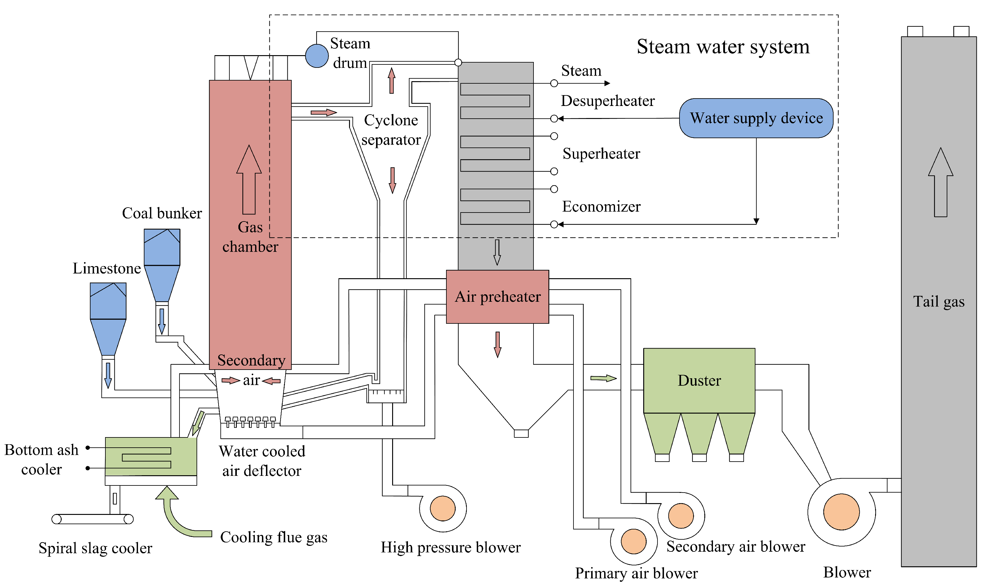
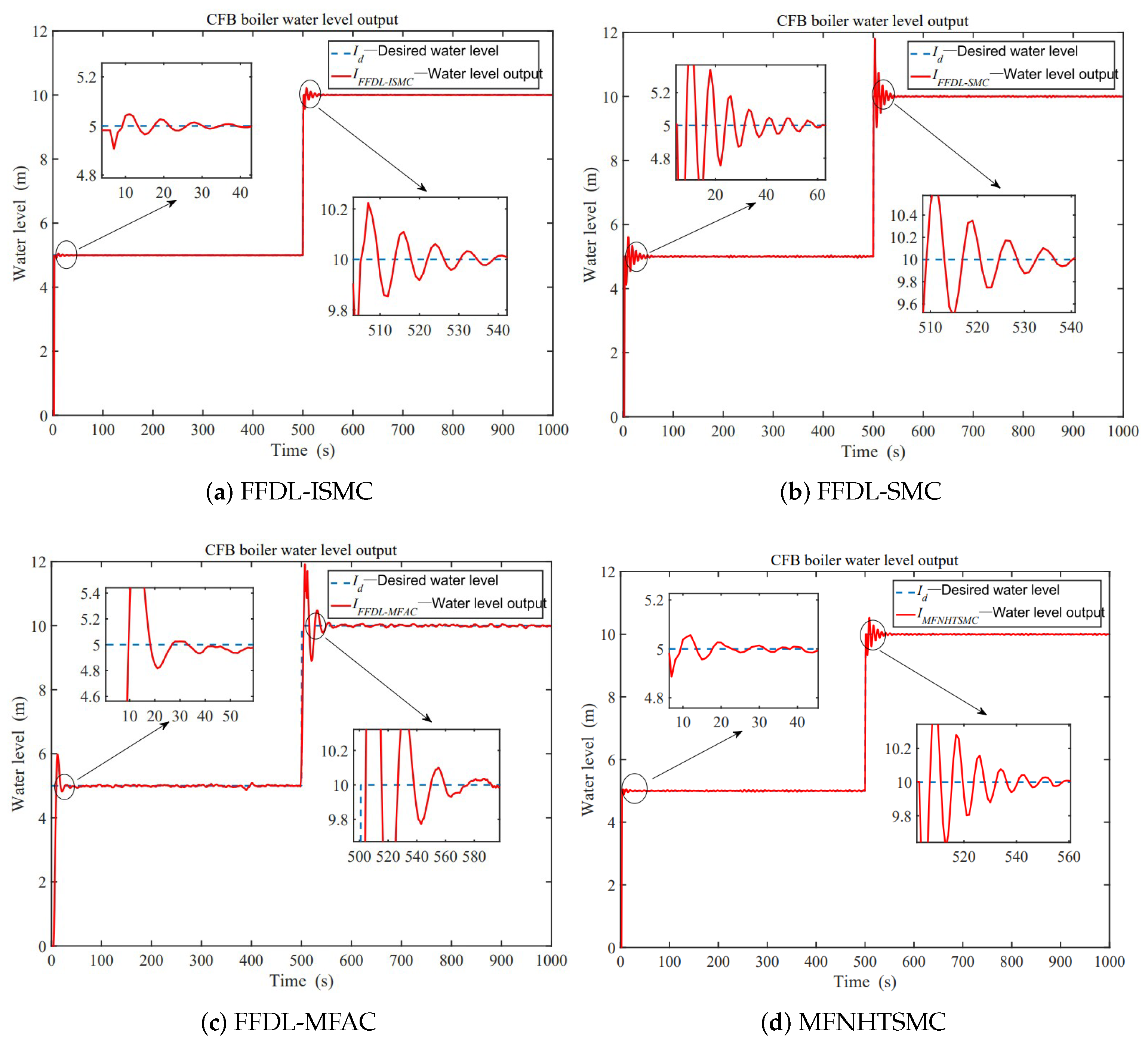
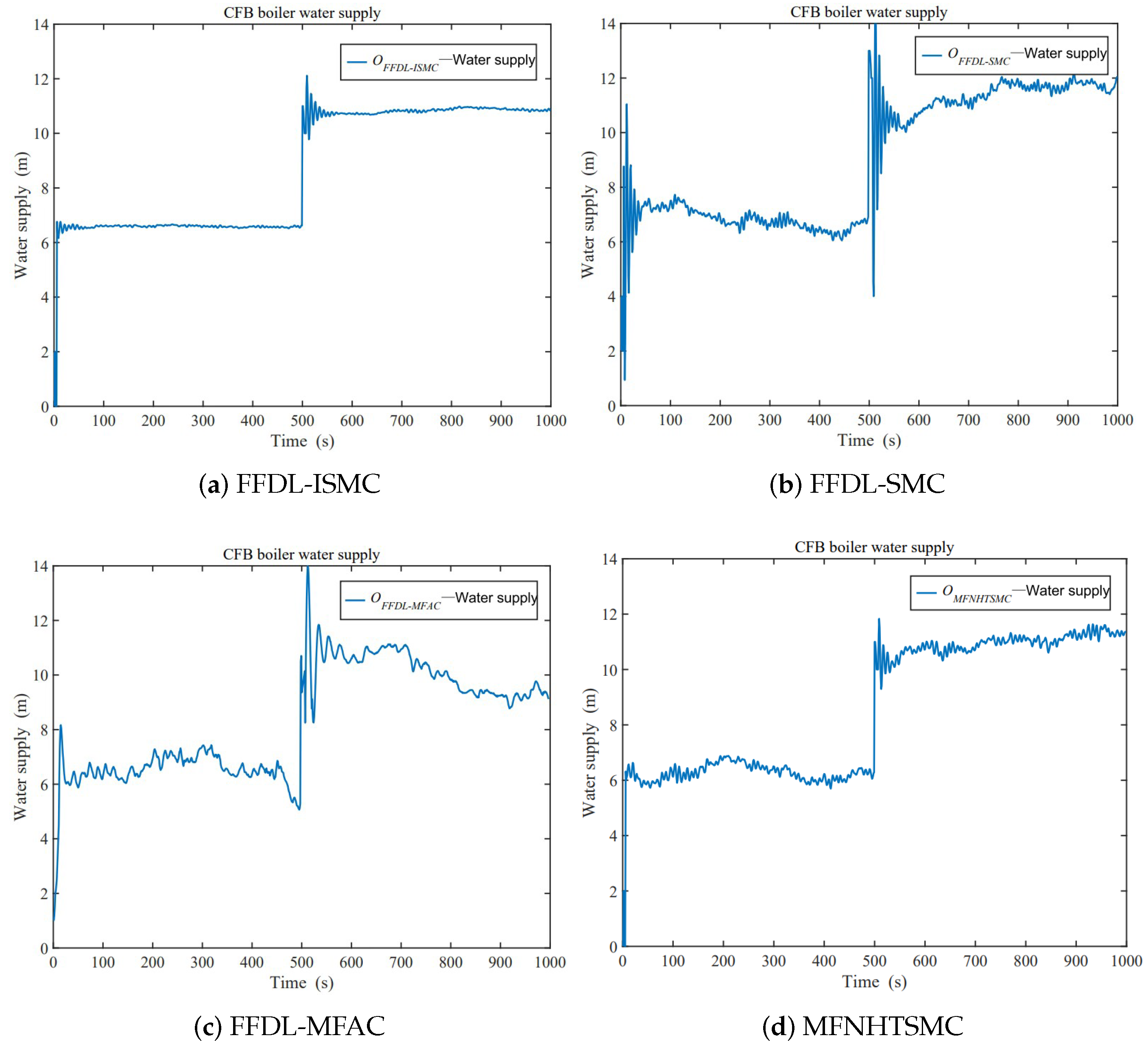
4.2. Experiment 2: Water-Level Control of CFB

The second group of experiments selected the water level of the steam drum in a CFB boiler as the research object. This simulation study demonstrates the effectiveness and application prospects of ISMC based on an FFDL data model.
The bubble water-level system of a CFB boiler refers to an important set of equipment and technology used to control the boiling state and monitor the water level in the boiler. CFB is an efficient and low-polluting form of boiler, characterized by the circulation and fluidization of particulate materials to achieve the combustion process. The bubble water-level system plays a role in monitoring and controlling the internal water level of fluidized bed boilers, ensuring their normal operation and safe operation. Specifically, the bubble water-level system mainly consists of the following components:
(1)
Water-level measurement sensor: used to detect changes in the water level inside the CFB boiler and convert the signal into an electrical signal sent to the control system, usually using pressure or a capacitance-type water-level sensor.
(2)
Control system: receive the water-level signal sent by the sensor, and according to the difference between the set value and the actual value, automatically adjust the amount of supply water or discharge steam in order to maintain the water level in the safe range.
(3)
Water-supply system: according to the signal of the control system, adjust the working status and water inflow of the water-supply pump to maintain the level inside the CFB boiler.
(4)
Exhaust system: the exhaust valve is adjusted to control the discharge or recovery of steam in order to maintain the airtightness and stable working conditions of the CFB.
The design and operation of the CFB boiler system plays an important role in improving the boiler efficiency, safe operation as well as reducing energy consumption and pollutant emissions.
The goal of controlling the steam-water system of a CFB boiler is to track the boiler feedwater flow rate and maintain the steam temperature within a given range while also ensuring the safety of the boiler and the stability of the steam turbine. By monitoring the water level and automatically controlling the water supply and steam discharge, it can ensure the normal operation of the CFB boiler and effectively prevent boiler accidents caused by too high or too low water levels. In the steam-water system of a CFB boiler (as shown in Figure 5), the steam-water system in the red-dashed box in Figure 5 is simplified to the flow diagram in Figure 6.
Since the physical properties of the boiler body change with time, the turbine water-level system is regarded as a slow time-varying system. Due to the difference in boiler tank capacity and volume, it takes a short time for the change in valve position to be reflected in the change in water level, which shows that there is a time delay in the system, and there is also the problem of interference in the system. Overall, the control problem of the steam-drum water level not only needs to solve the problem of nonlinear and difficult modeling, but also the problem of accompanying disturbances [30,31]. Above all, the turbine water-level system does not have an accurate model and is accompanied by disturbances.
The balance between boiler load and water supply is represented by the drum water level in CFB boilers. Therefore, it is crucial to maintain the water level at an acceptable working area in order to guarantee the stability and efficiency of the boiler operation.
In this example, the simulation model of the three-equilibrium control system of the turbine water level is based on the CFB boiler of type DHX25-1.25-AII, whose rated evaporation capacity is 25 t/h and rated pressure is 1.25 MPa; the physical platform is shown in Figure 7. It can be seen from the above that the two main factors of the water supply and the amount of steam have the greatest influence on the change in the turbine water level. This paper considers the impact of water supply on the water level of the steam drum, and there exists a dynamic mathematical model for this object as follows [32,33,34]:
G ( s ) = k T s ( T d s + 1 )
where G ( s ) is the control system’s transfer function, s is a complex variable in the transfer function, k is the proportional coefficient and T is the pure lag time under the water-supply disruption. T d is the water-level reaction time.
Remark 3.
It is worth noting that the mathematical model of the boiler water level used in this paper is merely an empirical model, and building a dynamic model that fully represents the system characteristics is actually quite challenging. On the other hand, there are complex actuators present in the boiler system, which have been collectively considered as part of an empirical model. The transfer function of the system can be transformed into a difference equation. Identify the system parameters using the least square method with the forgetting factor, and the mathematical model of the system is obtained.
The parameters are taken as T = 40 s and T d = 36 s . The parameters of the FFDL-ISMC and FFDL-SMC controllers are set to H ^ 1 ( 1 ) = H ^ 2 ( 1 ) = diag { 0.46 , 0.6 , 0.46 } , η = 0.75 , μ = 0.9 , β = 0.05 , θ = 0.2 , c 1 = 0.55 , c 2 = 0.35 , L I = 1 , L O = 1 , α = 0.5 . The FFDL-MFAC parameters are set to H ^ 1 ( 1 ) = H ^ 2 ( 1 ) = diag { 0.46 , 0.6 , 0.46 } , η = 0.75 , μ = 1 , θ = 0.2 , L I = 1 , L O = 1 . The MFNHTSMC method parameters are set to λ 1 = 12 , λ 2 = 2 , g 1 t 1 = 7 3 , g 2 t 2 = 5 3 , ε 1 = 0.02 , ε 2 = 0.005 [35]. The principle of FFDL-ISMC drum water-level control is shown in Figure 8.
Figure 9 shows the boiler bubble water-level output of the FFDL-MFAC, FFDL-SMC, MFNHTSMC and FFDL-ISMC methods, while Figure 10 shows the corresponding water-level output error. The performance indicators are summarized in Table 2. From the two sets of figures and Table 2, it is evident that the proposed FFDL-ISMC method not only has fast tracking characteristics but also effectively suppresses the influence of external disturbances, thereby maintaining a stable water-level height and exhibiting a superior tracking performance compared to the FFDL-MFAC, FFDL-SMC and MFNHTSMC methods.
The specific analyses are as follows: The water-level setting error range of the FFDL-ISMC method is within [ 0.221 m, 0.518 m], and the tracking accuracy is high, while the water-level errors of the FFDL-MFAC and FFDL-SMC methods are between [ 1.983 m, 1.498 m] and [ 1.817 m, 1.102 m], respectively. For the rise time, as shown in Table 2, the FFDL-ISMC method is nearly a quarter of FFDL-SMC and nearly half of FFDL-MFAC. The FFDL-ISMC method’s adjustment time is less than that of the FFDL-MFAC method and is almost exactly half that of the FFDL-SMC method. The MAE and MSE obtained by the FFDL-ISMC technique are substantially smaller than those obtained by the FFDL-MFAC and approximately half as large as those obtained by the FFDL-SMC method, indicating that it has more precision and stability. The chattering of the FFDL-ISMC method is reduced compared with that of the FFDL-SMC and MFNHTSMC methods.
Additionally, it is evident from Figure 9 and Figure 10 that the FFDL-ISMC method can still respond faster to the expected signal even under changing operating conditions (at the 500th second), and the chattering phenomenon is significantly better than the FFDL-SMC method, enabling better monitoring of the specified boiler bubble water level. This supports the effectiveness and excellence of the suggested approach even more.
Figure 11 shows the variation curves of the water-supply inputs of the FFDL-MFAC, FFDL-SMC, MFNHTSMC and FFDL-ISMC methods. It is easy to see that the water supply of the FFDL-MFAC and FFDL-SMC methods were in the process of large fluctuations, and the peak value is more than 14 m; thus, it is significantly impacted by the disruption and is vulnerable to significant or even minor issues. Additionally, adjusting the feedwater level frequently will put a lot of strain on the system’s parts. In contrast, the FFDL-ISMC method maintains the feedwater quantity within a reasonable working range with small variations. In addition, when the working conditions change, the control input of this method can also respond quickly.
The convergence of the input and output signals is demonstrated to further improve the application of the MFAC method in adjoint noise-interference systems in this chapter, which also proposes an ISMC method based on a data model for systems with adjoint noise interference. Simultaneously, experiments are conducted in various simulation environments, and the experimental findings demonstrate that, under various simulation conditions, the output error of the control method proposed in this chapter is clearly better than that of the original method, and it has the characteristics of quick responses and slight overshooting. The MFAC and SMC methods largely maintain their quick response times and robustness.

5. Conclusions

An improved ISMC scheme is proposed for the boiler water-level-control system. The algorithm is based on an FFDL model, and a discrete ISMC law is designed. The control scheme is designed to utilize only the input and output data without model information. After providing a stability proof analysis of the proposed method, in the special-equipment testing facility, the control problem of the DHX25-1.25-AII CFB boiler-drum water level is analyzed, along with the efficacy and viability of the enhanced-control approach. When the working conditions of the CFB system change, it can also respond quickly. The specific performance is as follows for the FFDL-ISMC method:
(1)
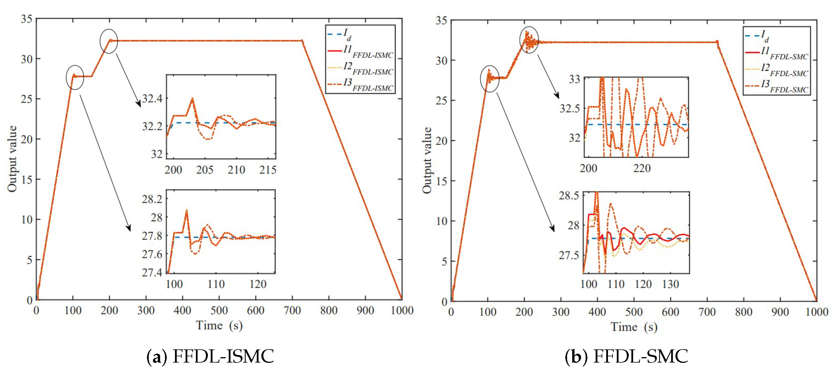
The FFDL-ISMC method improves the tracking speed and the fast-response characteristics of the MFAC strategy.
(2)
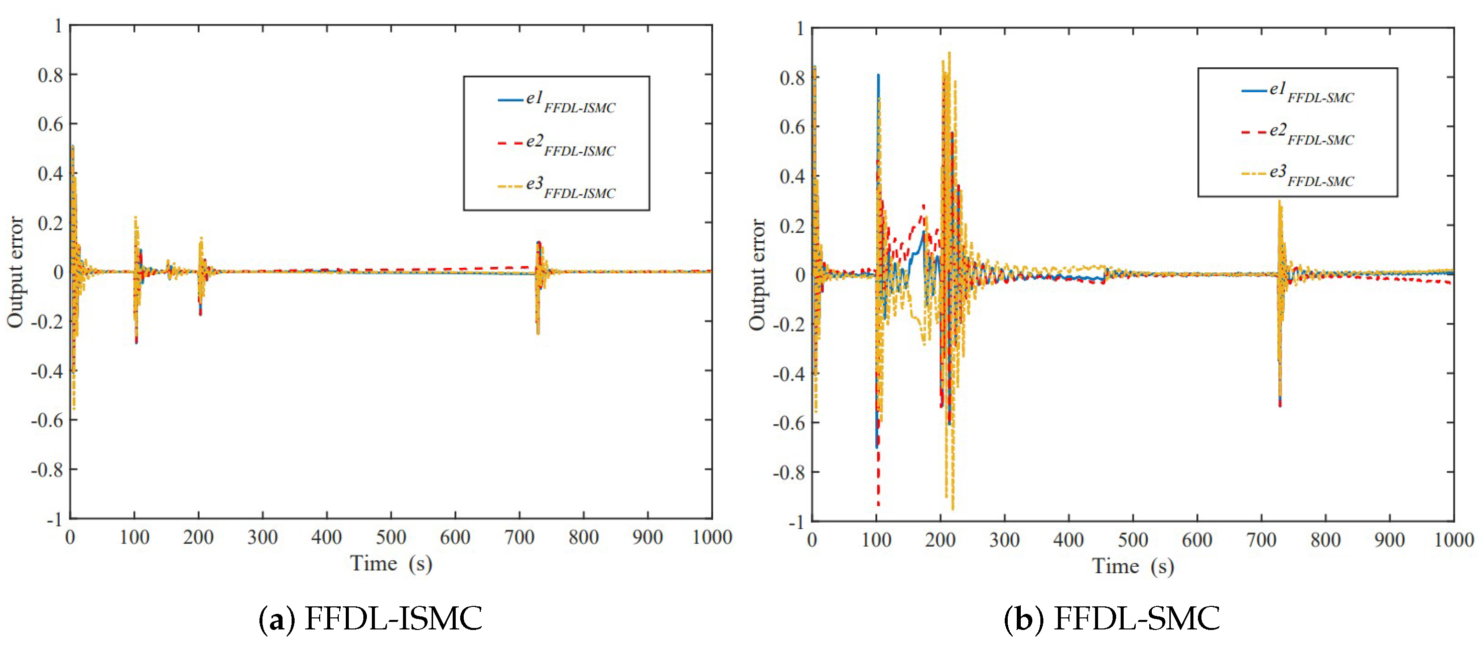
Compared with the FFDL-MFAC and FFDL-SMC methods, the FFDL-ISMC method provides higher accuracy and better stability. The FFDL-ISMC method is still able to respond faster to the feedback under variable operating conditions, thus better tracking the given boiler bubble level.
(3)
The FFDL-ISMC method maintains the feedwater level within a reasonable operating range with little variation. When the working conditions change, it can also respond quickly.
This paper designs an improved adaptive ISMC and verifies its effectiveness in practical systems through a transfer function model of the boiler-drum water level. Future research will consider the effects of two main factors: the impact of water supply and steam flow on the changes in the drum water level.

Author Contributions

Conceptualization, Z.S. and F.X.; methodology, F.X. and Z.S.; software, F.X. and Y.W.; validation, F.X. and Z.S.; formal analysis, Z.S.; resources, F.X.; writing—original draft preparation, F.X. and Z.S.; supervision, Z.S.; funding acquisition, F.X., J.X. and Z.S. All authors have read and agreed to the published version of the manuscript.

Funding

This research was funded by the Quzhou City Science and Technology Plan project (2023K263, 2023K265, 2023K045), the General Research Project of the Zhejiang Provincial Department of Education (2023) (Y202353440, Y202353289), and Quzhou Vocational and Technical College university-level scientific research project (QZYZ2305-2023).

Institutional Review Board Statement

Not applicable.

Informed Consent Statement

Not applicable.

Data Availability Statement

The data presented in this study are available in the article.

Conflicts of Interest

The authors declare no conflict of interest.

References

  1. Yang, Z.H.; He, Z.; Zhang, X.G.; Jiang, X.; Jin, Z.H.; Li, J.P.; Ma, L.; Wang, H.L.; Chang, Y.L. In-situ gas flow separation between biochar and the heat carrier in a circulating fluidized bed reactor for biomass pyrolysis. Chem. Eng. J. 2023, 472, 145099. [Google Scholar] [CrossRef]
  2. Xu, J.L.; Xu, F.; Wang, Y.L.; Sui, Z. An Improved Model-Free Adaptive Nonlinear Control and Its Automatic Application. Appl. Sci. 2023, 13, 9145. [Google Scholar] [CrossRef]
  3. Zhou, L.; Li, Z.-Q.; Yang, H.; Fu, Y.-T. Data-driven integral sliding mode control based on disturbance decoupling technology for electric multiple unit. J. Frankl. Inst. 2023, 360, 9399–9426. [Google Scholar] [CrossRef]
  4. Li, H.T.; Zheng, S.Q.; Ren, H.L. Self-correction of commutation point for high-speed sensorless BLDC motor with low inductance and nonideal back EMF. IEEE Trans. Power Electron. 2016, 32, 642–651. [Google Scholar] [CrossRef]
  5. Song, L.L.; Sun, W.L.; Liu, H. Fuzzy Adaptive PID Control of Drum Water Level in Boiler. Ind. Control. Comput. 2021, 34, 74–76. [Google Scholar]
  6. Zhen, L.C.; Gao, X. Research of Incomplete Differential PID Control in Boiler Water System. Boil. Technol. 2007, 4, 11–14. [Google Scholar]
  7. Guo, K. Design and Simulation of Cascade Fuzzy Control System for Boilers. Sci. Discov. 2020, 7, 446–452. [Google Scholar]
  8. Grin, E.A.; Panfilov, D.N. Monitoring the Percentage of Service Life Usage for Unheated High-Temperature Elements of Boilers. Therm. Eng. 2023, 70, 630–638. [Google Scholar] [CrossRef]
  9. Liu, T.; Zhang, S. Simulation and Research of CFB Boiler Level Control System Based on DMC-PID Algorithms. Mod. Ind. Econ. Informationization 2019, 9, 4–8. [Google Scholar]
  10. Zhou, L.; Li, Z.Q.; Yang, H.; Fu, Y.T.; Yan, Y. Data-Driven Model-Free Adaptive Sliding Mode Control Based on FFDL for Electric Multiple Units. Appl. Sci. 2022, 12, 10983. [Google Scholar] [CrossRef]
  11. Ma, Y.S.; Che, W.W.; Deng, C. Distributed model-free adaptive control for learning nonlinear MASs under DoS attacks. IEEE Trans. Neural Netw. Learn. Syst. 2021, 34, 1146–1155. [Google Scholar] [CrossRef] [PubMed]
  12. Hou, Z.S. Nonlinear System Parameter Identification, Adaptive Control and Model Free Adaptive Learning Control. Ph.D. Thesis, Northeastern University, Beijing, China, 1994. [Google Scholar]
  13. Jiang, Q.Q.; Liao, Y.L.; Cheng, C.S. Unmanned surface vessel heading control of model-free adaptive method with variable integral separated and proportion control. Int. J. Adv. Robot. Syst. 2019, 16, 141–149. [Google Scholar] [CrossRef]
  14. Wang, H.J.; Hou, Z.S. Model-free adaptive fault-tolerant control for subway trains with speed and traction/braking force constraints. IET Control. Theory Appl. 2020, 14, 1557–1566. [Google Scholar] [CrossRef]
  15. Moreno-Gonzalez, M.; Artuñedo, A.; Villagra, J.; Join, C.; Fliess, M. Speed-Adaptive Model-Free Path-Tracking Control for Autonomous Vehicles: Analysis and Design. Vehicles 2023, 5, 698–717. [Google Scholar] [CrossRef]
  16. Li, S.J.; Xu, C.Q.; Liu, J.L.; Xu, Z.Q.; Meng, F.B. Tracking control of ships based on ADRC-MFAC. Chin. J. Ship Res. 2023, 18, 1–10. [Google Scholar] [CrossRef]
  17. Pan, X.L.; Xian, B. Model-free adaptive robust control design for a small unmanned helicopter. Control. Theory Appl. 2017, 34, 1171–1178. [Google Scholar]
  18. Zhen, X.J.; Ding, M.; Wu, H.L.; Guo, M. Model-free adaptive control of cable-driven continuum manipulator. J. Huazhong Univ. Sci. Technol. (Nat. Sci. Ed.) 2023, 51, 116–121. [Google Scholar]
  19. Wang, X.F.; Li, X.; Wang, J.H. Active Interaction Exercise Control of Exoskeleton Upper Limb Rehabilitation Robot Using Model-free Adaptive Methods. Acta Autom. Sin. 2016, 42, 1899–1914. [Google Scholar]
  20. Wei, H.; Jie, T. On Simulation for Coal Mine Belt Servo System Based on MFAC. Comput. Simul. 2014, 31, 373–376. [Google Scholar]
  21. Rongmin, C.; Hongwei, L. Model-free adaptive control on linear motor servo system. J. Beijing Inf. Sci. Technol. Univ. 2012, 27, 39–44. [Google Scholar]
  22. Hu, Y.M.; Li, G.Q.; Zhang, J.L. Revamping of parameter input of MFAC and utilization in gas fractionation unit. CIESC J. 2015, 66, 4076–4084. [Google Scholar]
  23. Dong, N.; Lv, W.; Zhu, S.; Li, D. Anti-noise model-free adaptive control and its application in the circulating fluidized bed boiler. Proc. Inst. Mech. Eng. Part-J. Syst. Control. Eng. 2021, 235, 1472–1481. [Google Scholar] [CrossRef]
  24. Zhu, M.S.; Liu, J.M.; Hu, X.H.; Yu, S.; Xu, S.C.; Ye, Z.H. Research on Model Free Adaptive Control of Boiler Water Circulation System. J. Chongqing Univ. Technol. (Natural Sci.) 2019, 33, 214–220. [Google Scholar]
  25. Dong, N.; Lv, W.; Zhu, S.; Gao, Z.; Grebogi, C. Model-free adaptive nonlinear control of the absorption refrigeration system. Nonlinear Dyn. 2022, 107, 1623–1635. [Google Scholar] [CrossRef]
  26. Wang, Y.S.; Hou, M.D. Model-free adaptive integral terminal sliding mode predictive control for a class of discrete-time nonlinear systems. ISA Trans. 2019, 93, 209–217. [Google Scholar] [CrossRef] [PubMed]
  27. Xu, Y.T.; Wu, A.G. Integral sliding mode predictive control with disturbance attenuation for discrete-time systems. IET Control. Theory Appl. 2022, 16, 1751–1766. [Google Scholar] [CrossRef]
  28. Ma, Y.S.; Che, W.W.; Deng, C. Dynamic event-triggered model-free adaptive control for nonlinear CPSs under aperiodic DoS attacks. Inf. Sci. 2022, 589, 790–801. [Google Scholar] [CrossRef]
  29. Xiong, S.S.; Hou, Z.S. Model-free adaptive control for unknown MIMO nonaffine nonlinear discrete-time systems with experimental validation. IEEE Trans. Neural Netw. Learn. Syst. 2022, 33, 1727–1739. [Google Scholar] [CrossRef]
  30. Dong, N.; Zhu, S. Model-free Adaptive De-noising Control and Its Application. J. Hunan Univ. (Nat. Sci.) 2020, 47, 74–81. [Google Scholar]
  31. Nie, X.; Xie, H.Y.; Yang, D.; Liu, H.; Zhou, K.; Zhou, Z.P.; Li, Y.H.; Liu, Z.G. Safety analysis for boiler thermal-hydraulic circulation with severe peak load regulation of a CFB unit. J. Cent. South Univ. (Sci. Technol.) 2022, 53, 2766–2776. [Google Scholar]
  32. Ma, Y.F.; Niu, F.F.; Lv, J.F.; Jin, X.; Ma, H. Study of controlling thermal deviation in platen superheaters of a CFB boiler by utilizing header effect. J. Cent. South Univ. (Sci. Technol.) 2021, 52, 4454–4463. [Google Scholar]
  33. Huang, S.Z.; Li, X.S. Research and application on bed material preparation system of CFB boiler. Int. J. Energy Power Eng. 2020, 9, 108–114. [Google Scholar]
  34. Zhu, S. Research on Improve Model-Free Adaptive Control and its Application. Master’s Thesis, Tianjin University, Tianjin, China, 2019. [Google Scholar] [CrossRef]
  35. Zhao, K.; Liu, W.; Liu, Z.; Jia, L.; Huang, G. Model-Free High Sliding Mode Control for Permanent Magnet Synchronous Motor. Trans. China Electrotech. Soc. 2023, 38, 1472–1485. [Google Scholar] [CrossRef]
Figure 1. The FFDL-ISMC algorithm.
Applsci 13 13094 g001
Figure 2. Control methods output curve.
Applsci 13 13094 g002
Figure 3. Control methods output error curve.
Applsci 13 13094 g003
Figure 4. Control methods input curve.
Applsci 13 13094 g004
Figure 5. CFB system.
Applsci 13 13094 g005
Figure 6. The simplified CFB system.
Applsci 13 13094 g006
Figure 7. CFB boiler experiment platform.
Applsci 13 13094 g007
Figure 8. FFDL-ISMC of CFB system.
Applsci 13 13094 g008
Figure 9. Control-methods system output curve.
Applsci 13 13094 g009
Figure 10. Control-methods system output error curve.
Applsci 13 13094 g010
Figure 11. Control methods’ system-input curve.
Applsci 13 13094 g011
Table 1. Performance indexes of each control method.
MethodsFFDL-SMCFFDL-ISMC
Rise time (s)63
Adjust time (s)3210
MAE 3.32 × 10 2 8.15 × 10 3
MSE 1.73 × 10 2 2.27 × 10 3
Table 2. Control schemes’ performance indexes.
MethodsFFDL-MFACFFDL-SMCFFDL-ISMCMFNHTSMC
Rise time (s)91544
Adjust time (s)75583535
MAE 9.66 × 10 2 6.27 × 10 2 3.14 × 10 2 4.48 × 10 2
MSE 1.15 × 10 1 6.62 × 10 2 2.43 × 10 2 5.37 × 10 2
Disclaimer/Publisher’s Note: The statements, opinions and data contained in all publications are solely those of the individual author(s) and contributor(s) and not of MDPI and/or the editor(s). MDPI and/or the editor(s) disclaim responsibility for any injury to people or property resulting from any ideas, methods, instructions or products referred to in the content.

