Comparing Artificial Intelligence Algorithms with Empirical Correlations in Shear Wave Velocity Prediction

Abstract

Accurate estimation of shear wave velocity ($V_s$) is crucial for modeling hydrocarbon reservoirs. The $V_s$ values can be directly measured using the Dipole Shear Sonic Imager data; however, it is very expensive and requires specific technical considerations. To address this issue, researchers have developed different methods for $V_s$ prediction in underground rocks and soils. In this study, the well logging data of a wellbore in the Iranian Aboozar limestone oilfield were used for $V_s$ estimation. The $V_s$ values were estimated using five available empirical correlations, linear regression technique, and two machine learning algorithms including multivariate linear regression and gene expression programming. Those values were compared with the real $V_s$ data. Furthermore, three statistical indices including correlation coefficient ($R^2$), root mean square error ($RMSE$), and mean absolute error ($MAE$) were used to evaluate the effectiveness of the applied techniques. The mathematical correlation obtained by the GEP algorithm delivered the most accurate $V_s$ values with $R^2$ = 0.972, $RMSE$ = 0.000290, and $MAE$ = 0.000208. Compared to the available empirical correlations, the obtained correlation from the GEP approach uses multiple parameters to estimate the $V_s$, thereby leading to more precise predictions. The new correlation can be used to estimate the $V_s$ values in the Aboozar oilfield and other geologically similar reservoirs.

1. Introduction

Shear wave velocity is an indispensable parameter in geoscience with numerous conventional and emerging applications. The conventional applications include earthquake engineering [1], geotechnical site characterization [2,3], reservoir characterization [4,5], and groundwater resource assessment [6,7]. Moreover, the emerging applications of shear wave velocity are geothermal energy exploration [8], landslide hazard assessment [9], carbon capture and storage (CCS) [10], geohazard assessment in offshore environments [11], and deep earth exploration [12].

Accurate estimation of $V_s$ is highly crucial in reservoir modeling. In fact, the $V_s$ values are chiefly used to create the geomechanical models of reservoirs. Those models are highly applicable in all stages of hydrocarbon production. For instance, some applications are pore pressure prediction, wellbore stability analysis, casing failure analysis, land subsidence prediction, reservoir depletion analysis, etc.

Generally, $V_s$ determination methods can be categorized into six general categories based on their underlying principles and approaches.

Table 1. Different types of $V_s$ measurement methods with their respective pros and cons.

${\mathit{V}}_{\mathit{s}}$ Measurement Method	Advantages	Disadvantages
Laboratory Core Analysis	Provides accurate measurements. Allows detailed core sample analysis. Offers insights into rock properties.	Expensive and time-consuming. Limited to a small number of samples. May not replicate in situ conditions.
Geophysical Well Logging and In Situ Measurements	Provides direct measurements. Suitable for real-time well logging.	Limited to borehole locations. Tools and data acquisition can be costly.
Empirical and Correlation-Based Methods	Simplicity and ease of application. Uses readily available well log data.	Limited accuracy, relying on correlations. Applicability may be region-specific.
Theoretical and Physics-Based Models	Consider physical properties. Provides insights into rock behavior.	Complex and data-intensive. Requires a wide range of input parameters.
Data-Driven and Machine Learning Techniques	Handles complex data. Learning from diverse datasets.	Needs extensive, high-quality training data. Models may not always be interpretable.
Seismic and Geostatistical Approaches	Provides large-scale $V_s$ estimations. Characterization beyond wellbore.	Limited to seismic data availability. Inversion and modeling can be computationally intensive.

presents the general categories of $V_s$ prediction methods along with their merits and demerits. The choice of method depends on the specific project goals, data availability, and the trade-offs between accuracy, cost, and complexity.

Traditional methods of $V_s$ prediction, such as laboratory testing and borehole measurements, are time-consuming, expensive, and often impractical for large-scale studies [13]. Moreover, the only wireline log tool to record the shear wave velocity is the Dipole Shear Sonic Imager (DSI) log, which is very expensive. For this purpose, various empirical correlations have been introduced for $V_s$ estimation in different rocks [14,15,16,17,18,19,20,21,22,23,24,25,26,27,28,29,30,31,32,33]. For instance, some well-known correlations for $V_s$ prediction in carbonate rocks can be found in Castagna et al. [18], Carroll [15], Wadhwa et al. [27], Pickett [14], and Anselmetti and Eberli [23]. Regardless of the rock type, those empirical correlations usually used one parameter to estimate the $V_s$. It is clear that each extracted empirical correlation has its advantages and drawbacks. For example, Wantland used Poisson’s ratio to predict the $V_s$ values in reservoir rocks [32]. Nevertheless, the Poisson’s ratio of rocks usually varies remarkably, and thus, the accuracy of the estimated values of $V_s$ might be affected [15,29].

In the past few years, the AI techniques have been widely used in geoscience applications such as reservoir characterization [34], geotechnics [35,36,37], mining exploration [38], earthquake engineering [39,40], etc. Two of the frequent AI techniques are the MLR and GEP. MLR is a statistical method used in the field of machine learning and statistics to model the relationship between a dependent variable and two or more independent variables [41]. In fact, it is an extension of simple linear regression, which models the relationship between a dependent variable and a single independent variable. On the other side, the GEP approach has been broadly used in engineering projects, from hydraulics [42] to reservoir characterization [43]. GEP is a specific variant of genetic programming (GP) that emphasizes the representation and evolution of linear or tree structures using a process called gene expression. Generally, in GP, a population of candidate solutions (programs) is evolved over generations through the application of genetic operators such as mutation, crossover, and selection [44].

The MLR and GEP techniques were also applied to predict the $V_s$ in rocks [45,46,47,48,49,50,51]. Upom et al. used the MLR and an ensemble (EN-PSO) model to predict the $V_s$ values in soils [45]. In their work, the independent variables were the soil type, depth, and standard penetration resistance. They reported that both MLR and EN-PSO models predicted the $V_s$ values with high accuracy. In another study, Ataee et al. estimated the $V_s$ of soils by applying MLR and artificial neural network (ANN) [46]. It was declared that the ANN technique delivered more precise results. The MLR technique was also applied for $V_s$ prediction in hydrocarbon reservoirs by some researchers [47,48]. Shi and Zhang evaluated the capability of MLR, multivariable polynomial regression, deep neural network (DNN), and random forest in $V_s$ prediction for hydrocarbon reservoirs [48]. According to the obtained results, the random forest technique exhibited a better predictive capability than others.

Behnia et al. used the GEP and ANFIS techniques to extract mathematical relations for $V_s$ prediction in limestone rocks in Iran [49]. In their study, the input parameters were density, porosity, and compressional wave velocity ($V_p$). Both techniques showed remarkable performance in predicting accurate $V_s$ values. In another study, Gullu predicted the $V_s$ values in soils using GEP and ANN techniques to characterize the potential of earthquakes in different sites in California, USA [50]. It was concluded that both techniques were promising for $V_s$ prediction. In a similar investigation, Khazaee et al. used the GEP technique to determine the soil types based on the $V_s$ values [51]. A mathematical relationship was extracted and proposed for $V_s$ estimation. Such a relationship exhibited an excellent performance for $V_s$ estimation in soils.

In this study, the well logging data obtained from a vertical wellbore in Aboozar limestone oilfield were used to estimate the $V_s$ values. The Aboozar oilfield is situated 74 km away from Kharg Island in the Persian Gulf. The $V_s$ estimation was carried out using five available empirical correlations, LR, and two AI algorithms including MLR and GEP. The main objective of the research was to compare the performance of those different techniques in $V_s$ estimation. For this purpose, the $V_s$ values estimated by each technique were validated and compared with the real $V_s$ data. The additional target was to find a mathematical relationship capable of accurately predicting $V_s$ values in the oilfield. Based on the conducted research, the GEP algorithm delivered more accurate results than others. Hence, the corresponding mathematical relationship will be used for $V_s$ prediction in the oilfield. Compared to the available empirical methods which use only one parameter to estimate the shear wave velocity, the novel correlation extracted via the GEP technique considers four parameters to predict the $V_s$ values. This advantage results in more accurate predictions of $V_s$ values in the oilfield. It is noteworthy that the obtained mathematical relationship can be also used in other reservoirs containing identical geological conditions.

The structure of this article has been arranged as follows: Firstly, in Section 2.1, a brief description of the oilfield project is elaborated. Then, in Section 2.2, the raw well logging data are presented. Next, in Section 2.3.1, the linear correlations between the different well logging parameters and $V_s$ are extracted using the LR technique. Afterwards, in Section 2.3.2, the basic formulations related to the five applied empirical correlations are explained. Then, the basics of the MLR and GEP methods are described in Section 2.3.3 and Section 2.3.4, respectively. Thereafter, in Section 3, the findings derived from the conducted research are presented. Following that, Section 4 is dedicated to discussing the obtained results. Finally, in the Conclusions section, the article ends with a concise description about the key findings, results, future works, and implications.

2. Data and Methods

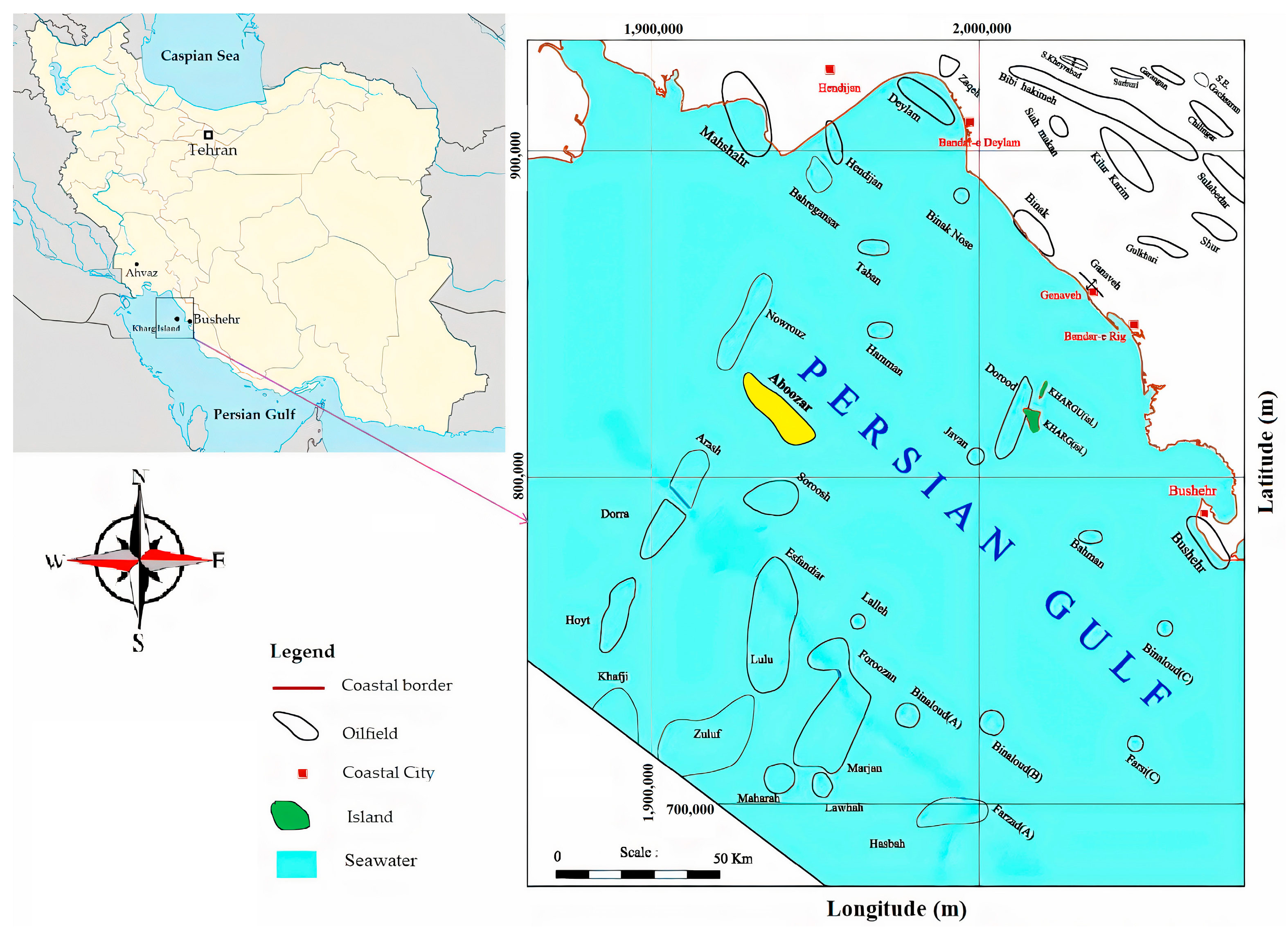
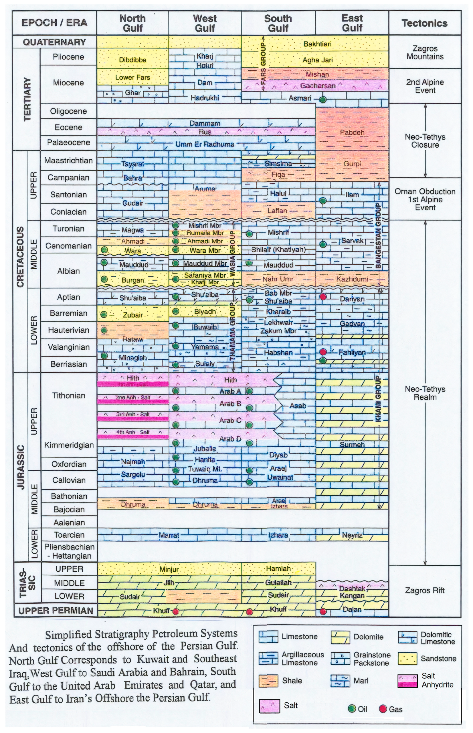
2.1. Project Description

In this research, the study area is the Aboozar oilfield located 74 km west of Kharg Island. Figure 1 shows the location of the Aboozar oilfield along with Kharg Island and other adjacent oilfields. For a better illustration, the Aboozar oilfield and Kharg Island have been shown in a yellow and green color, respectively. As shown in this figure, Aboozar oilfield is situated between the Nowrouz and Soroosh oilfields.

In 1959, the first exploration wellbore was drilled in the Aboozar oilfield. Further exploratory works were pursued until 1975. Subsequently, the oil production phase commenced in November 1976. The oilfield was initially operated by the Iran Pan American Company (IPAC), and it was then transferred to the Iranian Offshore Oil Company (IOOC) in 1979. Up to now, ten platforms with more than 140 vertical, deviated, and horizontal wellbores have been drilled in the oilfield. Those wellbores are connected to three main production platforms: AA, AB, and AC. Presently, a total of 90 wellbores are operating while the rest are inactive due to different technical issues. Based on the exploratory activities, it is estimated that the Aboozar oilfield contains 4 billion barrels of crude oil. The current production rate of the oilfield is around 200,000 barrels per day. The oil extracted from the platforms is transferred to Kharg Island through a 24-inch-diameter pipeline. It is noteworthy that in the Aboozar oilfield, more than one hundred people are currently working. Moreover, the depth of seawater in the area is nearly 40 m.

The main reservoir in this oilfield is the Asmari formation situated under the Gachsaran anhydrite caprocks. Figure 2 shows the simplified stratigraphy petroleum systems and tectonics offshore of the Persian Gulf. As shown in this figure, the Asmari formation is considered as the first oil-bearing formation in both the South Gulf and East Gulf sections. The East Gulf refers to the Iranian waters offshore of the Persian Gulf. Based on this figure, the Asmari formation contains Oligocene- and Miocene-aged carbonate and limestone rocks [52,53].

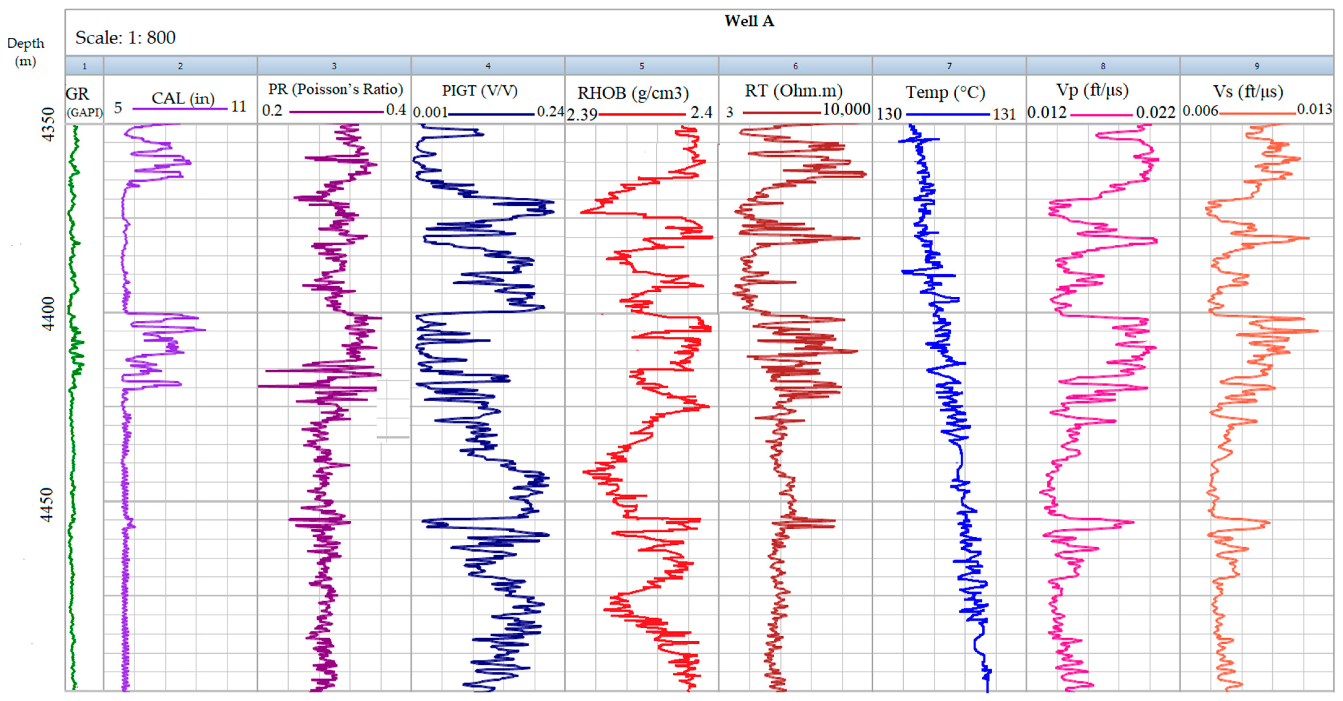
2.2. Well Logging Data

In this research, the well logging data pertinent to a vertical wellbore, called Well A, in the Aboozar oilfield were used as the raw data. The recorded data belonged to the limestone formations at a depth from 4350 m to 4500 m. The corresponding well logs are gamma ray log ($GR$), caliper log ($CAL$), Poisson’s ratio ($PR$), total porosity ($PIGT$), density log ($RHOB$), true formation resistivity log ($RT$), temperature ($TEMP$), compressional wave velocity ($V_p$), and shear wave velocity ($V_s$). Figure 3 illustrates the plot of the different well logging data used in the current research. It is noteworthy that the Poisson’s ratio values in the $PR$ log have been measured independently of the $V_s$ and $V_p$. Moreover, the rock density fluctuated between 2.39 g/cm³ and 2.40 g/cm³ for the entire profile. Therefore, it can be expressed that the rock density was relatively constant in our research.

2.3. Methodology

2.3.1. Linear Regression (LR)

To extract the correlations between $V_s$ and other parameters, the corresponding cross-plots for all well logs have been drawn in Figure 4.

Based on Figure 4, it can be seen that the $V_p$ and $PIGT$(porosity) logs show good correlations with the $V_s$ data. The linear correlation between the $V_s$ and $V_p$ was obtained as

$$V_s=0.45 V_p+0.001,$$

(1)

where $V_s$($\mathrm{ft}/\mathsf{\mu }\mathrm{s}$) and $V_p$ ($\mathrm{ft}/\mathsf{\mu }\mathrm{s}$) are shear and compressional wave velocities, respectively. Moreover, for the above equation, the $R^2$ was 0.95, the $RMSE$ was equal to 0.00032, and the $MAE$ was equal to 0.00029. Such a high correlation coefficient shows that Equation (1) is appropriate for predicting the $V_s$ in the Aboozar limestone oilfield. It is noteworthy that the $V_s$, $V_p$, and rock density can be utilized for estimation of the elastic moduli of different rocks [54,55].

The inclusion of linear regression in this study serves a dual purpose. Firstly, it allows for a baseline comparison with traditional linear methods, providing a clear contrast to highlight the superior predictive performance of our chosen nonlinear algorithms (gene expression programming and multivariate regression). Additionally, linear regression models offer inherent interpretability, contributing to a nuanced understanding of the predictive capabilities of both linear and nonlinear approaches. This choice facilitates a comprehensive analysis and comparison, demonstrating the advantages of employing nonlinear methods for predicting shear wave velocity while acknowledging the historical significance of linear regression in empirical correlations such as the Pickett equation.

2.3.2. Empirical Correlations

The previous studies conducted by the geomechanics and geophysics researchers have led to extraction of different empirical correlations to estimate the $V_s$ using other geological parameters. Each empirical correlation was proposed for a particular reservoir rock. In this research, the type of the reservoir rock is limestone; hence, only the well-known empirical correlations for limestone rocks have been used to estimate the $V_s$ in the Asmari formation (

Table 2. Empirical correlations related to estimation of $V_s$ in limestone reservoirs.

Correlation	Formula		Units
Castagna et al., 1998 [18]	$V_s=-0.05509 V_p{}^2+1.0168 V_p-1.0305$	(2)	$V_p$ ($\mathrm{km}/\mathrm{s}$) and $V_s$ ($\mathrm{km}/\mathrm{s}$)
Carroll, 1969 [15]	$V_s=0.937562 V_p{}^{0.82}$	(3)	$V_p$ ($\mathrm{kft}/\mathrm{s}$) and $V_s$ ($\mathrm{kft}/\mathrm{s}$)
Wadhwa et al., 2010 [27]	$V_s=1.09913326 V_p{}^{0.92}$	(4)	$V_p$ ($\mathrm{m}/\mathrm{s}$) and $V_s$ ($\mathrm{m}/\mathrm{s}$)
Pickett, 1963 [14]	$V_s=V_p/1.9$	(5)	$V_p$ ($\mathrm{ft}/\mathsf{\mu }\mathrm{s}$) and $V_s$ ($\mathrm{ft}/\mathsf{\mu }\mathrm{s}$)
Anselmetti and Eberli, 1993 [23]	$V_s=199 {\left(\gamma \right)}^{2.84}$	(6)	$V_s$ (m/s); $\gamma$ is density (g/cm3)

). Those empirical correlations included those of Castagna et al., Carroll, Wadhwa et al., Pickett, and Anselmetti and Eberli. It is noteworthy to mention that only the Anselmetti and Eberli correlation estimates the $V_s$ values using the rock density while the rest apply the compressional wave velocity ($V_p$) for $V_s$ estimation [14,15,18,23,27].

2.3.3. MLR Analysis

The MLR analysis is a statistical approach with only one dependent and many independent variables. MLR provides insights into the strength and direction of the relationships between the independent variables and the dependent variable [56,57,58]. In this approach, a relationship between the main function ($Y$) and the independent variable of $x_i$ is defined as

$$Y=f\left(x_i\right)$$

(7)

When $Y$ is defined as a linear function, the relationship is called the linear regression. Similarly, if $Y$ is defined as a nonlinear function of $x_i$, it is called the nonlinear regression [58].

The MLR approach delivers suitable predictive models for various surface and subsurface geoscience applications [58]. Consequently, in this research, the MLR approach was utilized to estimate the $V_s$. The general form of the approach is

$$Y=a_0+a_1{x}_1+\cdots +a_n{x}_n+C,$$

(8)

where $x_1,x_2,x_3,\dots .,x_n$ are the independent variables, $Y$ represents the dependent variable, and $a_0,a_1,a_2,a_3,\dots .,a_n$ are regression coefficients. The coefficients can be interpreted to understand the effect of each independent variable while holding others constant. Such coefficients are calculated by the least square method. Furthermore, the parameter of $C$ is a real number.

In the MLR analysis, the correlation coefficient,$R^2$, serves as a fitness indicator of the extracted relationship between the $Y$ and independent variables. The corresponding mathematical formula is

$$R^2=\frac{{{\displaystyle \sum }}_{i=1}^n{({\widehat{Y}}_i-\overline{Y})}^2}{{{\displaystyle \sum }}_{i=1}^n{(Y_i-\overline{Y})}^2}=1-\frac{{{\displaystyle \sum }}_{i=1}^n{(Y_i-{\widehat{Y}}_i)}^2}{{{\displaystyle \sum }}_{i=1}^n{(Y_i-\overline{Y})}^2},$$

(9)

where ${\widehat{Y}}_i$ and $Y_i$ represent the calculated value and real value of the $i$th sample of the dependent parameter, respectively. In addition, $\overline{Y}$ indicates the mean of the dependent parameter. When $R^2$ is close to 1, it means that there is a good correlation between the independent and dependent variables. Nevertheless, when $R^2$ approaches 0, it means that the fitness of the function is low. More technical details are available in the research published by Granian et al. [56].

An advantage of MLR is its simplicity, as it allows for the incorporation of multiple independent variables to capture complex relationships. Nevertheless, this flexibility can become a disadvantage when dealing with a large number of predictors, as MLR may be prone to overfitting. Overfitting occurs when the model fits the training data too closely, capturing noise and idiosyncrasies rather than the underlying patterns. Including too many predictors relative to the sample size can lead to a highly flexible model that performs well on the training data but fails to generalize effectively to new, unseen data. Regularization techniques, such as ridge regression or lasso regression, can be employed in MLR to address overfitting by imposing constraints on the coefficients, preventing them from reaching extreme values and promoting a more parsimonious model that generalizes better to new observations.

2.3.4. GEP Method

The GEP method was first introduced by Candida Ferreira in 2001. It is still considered as an applicable technique to set up complex computer programs and computational models [59,60]. Generally, those computer programs and models are sophisticated tree networks, exactly similar to the living organisms. The basis of the GEP method is identical to the genetic programming (GP) and genetic algorithms (GAs) approaches. In other words, the GEP method modifies the population of the initial individuals through the fitness evaluation process performed via one or more genetic operators [61].

The basic discrepancy between the GP, GAs, and the GEP approaches lies in the essence of the individuals; in the GP algorithm, the individuals represent the nonlinear beings which have miscellaneous dimensions and forms. On the other hand, the GAs incorporate the individuals as the linear strings with constant lengths. The GEP approach also applies the individuals as the linear strings with consistent length but it expresses them as the nonlinear beings with different dimensions and shapes.

To use the GEP method, generally, five elements are required: the terminal set, the function set, the fitness function, the control factors, and the stop criterion [60,62]. In GEP, solutions are represented as strings of symbols known as chromosomes. These chromosomes consist of genes, which are typically represented as mathematical or logical functions or operators. The solving process commences with the generation of a set of chromosomes in the initial population. Afterward, each chromosome is represented as the expression trees. These expression trees represent mathematical expressions or computer programs. GEP’s unique feature is its use of expression trees to represent solutions. Then, all individuals undergo the fitness evaluation operation.

GEP employs a genetic algorithm to evolve and improve the population of expression trees over generations. This process involves selection, recombination (crossover), mutation, and reproduction. Crossover involves the exchange of genetic material between two parent expression trees, resulting in two offspring. Mutation introduces random changes to the genes in an expression tree. Fitness functions are used to evaluate the performance of the expression trees. Through this, the best fitted individuals are selected and transferred to the next irritation. The surviving individuals are modified in each irritation, and the process continues until the stop criterion is met [61]. In Figure 5, the GEP algorithm flowchart has been depicted.

Therefore, in general, it can be said that the GEP algorithm uses the linear genomes as the genetic basis, as well as the operators such as mutation, crossover, recombination, inversion, and transposition. While it is typically advised to keep the mutation and inversion rates at low values within the range of 0.01 to 0.1, the transposition and recombination rates are commonly recommended to be in the moderate range of 0.1 to 0.4 [63].

The genomes are expressed by the chromosomes, and each chromosome is composed of genes which are translated to solve a complex problem. One of the advantages of GEP is its ability to discover mathematical relationships within data without prior knowledge of the functional form of the equations. It is particularly useful when dealing with complex, non-linear, or multidimensional data. GEP’s adaptability and capability to evolve both the structure and content of expressions make it a powerful tool for symbolic regression and automatic program generation. However, it may require careful parameter tuning and significant computational resources, especially for complex problems. For detailed information about the GEP algorithm see Ferreira’s book [63].

Although the GEP algorithm is a potent tool to predict the unknown variables, the overfitting issue may be a concern. In this research, to avoid overfitting, different strategies such as population diversity, selection of larger datasets, and formulation of precise fitness function were considered. It is worth mentioning that to avoid overfitting, the ensemble methods and regularization techniques such as penalizing complex programs or using techniques like Occam’s razor [64] can also be implemented [65]. The ensemble methods can improve generalization performance and reduce the impact of overfitting [66].

3. Results

3.1. Empirical Correlations

Shear wave velocity can be calculated using some existing empirical equations proposed by a number of researchers. In general, those empirical equations were developed for particular rock types. In the current study, the rock type of the reservoir is limestone. In Section 2.3.1, a number of available empirical correlations for limestone formations were recounted. In this research, at first, the values of $V_s$ were calculated using those equations, and then, those calculated values were compared with the real $V_s$ data obtained from the DSI log. Figure 6 shows the plot of the real $V_s$ log versus the graphs of $V_s$ predicted by those five existing empirical correlations.

Comparing the real $V_s$ data with the $V_s$ predicted by those five empirical correlations shows that the Pickett equation delivers the most accurate predictions of the $V_s$ values. Therefore, after the potential calibration, this empirical correlation can be deployed in the current oilfield.

Moreover, the values of the statistical indicators ($R^2$, $RMSE$, and $MAE$) were used to compare the accuracy of those empirical correlations. the simultaneous use of $R^2$, $RMSE$, and $MAE$ provides a more comprehensive and balanced evaluation of a predictive model, considering different aspects of its performance and helping to make more informed decisions in various contexts [67,68].

Table 3. The calculated values of $R^2$, $RMSE$, and $MAE$ for different empirical correlations.

Method	${\mathit{R}}^2$	$\mathit{R}\mathit{M}\mathit{S}\mathit{E}$	$\mathit{M}\mathit{A}\mathit{E}$
Castagna et al., 1998 [18]	0.49	1.02261	1.02161
Carroll, 1969 [15]	0.68	0.02358	0.02343
Wadhwa et al., 2010 [27]	0.67	0.01642	0.01627
Pickett, 1963 [14]	0.95	0.00042	0.00032
Anselmetti and Eberli, 1993 [23]	0.35	0.00825	0.00816

depicts the corresponding results. In this table, the values of $R^2$, $RMSE$, and $MAE$ related to all five empirical correlations have been tabulated.

According to Table 3, the Pickett equation has a better correlation coefficient, $RMSE$, and $MAE$ value. This matter can be clearly seen in Figure 6. Concerning the Anselmetti and Eberli equation, it can be observed that the predicted $V_s$ graph is a straight line, thereby calculating the $V_s$ as a constant value (also see Figure 6). In fact, the $V_s$ is a function of many other geomechanical parameters such as in situ stress, poroelastic properties, fluid content, etc., which cannot be represented only by rock density.

3.2. MLR Method

In well logging, each well log shows a series of the reservoir characteristics. If several well logs are used to determine the properties of a reservoir rock, it leads to more reliable results. Considering those characteristics, in this research, several well logs were deployed to estimate the values of $V_s$. At the beginning of the analysis, two logs including the $V_p$ and $PIGT$, which showed strong correlations with the $V_s$ data, were selected. Then, other logs were added one after another. In

Table 4. The calculated statistical indicators ($R^2$, $RMSE$, and $MAE$) values corresponding to the different MLR models.

Dataset	Input Parameters	${\mathit{R}}^2$	$\mathit{R}\mathit{M}\mathit{S}\mathit{E}$	$\mathit{M}\mathit{A}\mathit{E}$
Dataset 1	$V_p$ and $PIGT$	0.95	0.000986	0.000893
Dataset 2	$V_p$, $PIGT$, and $CAL$	0.96	0.000976	0.000899
Dataset 3	$V_p$, $PIGT$, $CAL$, and $PR$	0.96	0.000993	0.000954
Dataset 4	$V_p$, $PIGT$, $CAL$, $PR$, and $RT$	0.96	0.000969	0.000891
Dataset 5	$V_p$, $PIGT$, $CAL$, $PR$, $RT$, and $GR$	0.96	0.000969	0.000910
Dataset 6	$V_p$, $PIGT$, $CAL$, $PR$, $RT$, $GR$, and $RHOB$	0.96	0.000310	0.000252
Dataset 7	$V_p$, $PIGT$, $CAL$, $PR$, $RT$, $GR$, $RHOB$, and $TEMP$	0.96	0.000881	0.000764

, the $R^2$, $RMSE$, and $MAE$ values corresponding to seven datasets imported to the MLR models have been tabulated.

Comparing the results obtained from the different MLR models, it can be expressed that the correlation coefficients for all datasets were nearly equal to 0.96; however, Dataset 6 gave the lowest $RMSE$ and $MAE$ value. Therefore, this dataset is more appropriate than other datasets to derive an accurate estimation of the shear wave velocity from the MLR method. Ultimately, using Dataset 6, the following equation was extracted:

$$\begin{gathered} V_s=-0.1180+0.456290 V_p-0.000726 PIGT+0.000141 CAL- \\ 0.003617 PR+0.000001 RT-0.000005 GR+0.119900 RHOB, \end{gathered}$$

(10)

where $V_p$ ($\mathrm{ft}/\mathsf{\mu }\mathrm{s}$) and $V_s$ ($\mathrm{ft}/\mathsf{\mu }\mathrm{s}$) are compressional and shear wave velocities, respectively. Furthermore, $PIGT$ is porosity, $CAL$ (in) is the caliper log, $PR$ is the Poisson’s ratio, $RHOB$ (g/cm³) is density, $GR$ (GAPI) is gamma ray, and $RT$ (Ω·m) is the resistivity.

In Equation (10), it is evident that the coefficients for $RT$ and $GR$ parameters are notably smaller compared to the other parameters. This suggests a potential limited impact of these two parameters on the predicted $V_s$. To offer a more detailed understanding,

Table 5. Coefficients and ranges of parameters in Equation (10).

Parameter	Unit	Coefficient	Range
$V_p$	($\mathrm{ft}/\mathsf{\mu }\mathrm{s}$)	0.456290	0.0127–0.0205
$PIGT$	-	−0.000726	0.0036–0.2340
$CAL$	in	0.000141	5.6562–10.5145
$PR$	-	−0.003617	0.2121–0.3745
$RT$	Ω·m	0.000001	0.5456–7200
$GR$	GAPI	−0.000005	9.0195–65.0151
$RHOB$	g/cm3	0.119900	2.3955–2.3400

provides the coefficients and the respective ranges for each independent parameter incorporated in Equation (10). These coefficients reflect the sensitivity of the model to changes in each parameter. As observed, $RT$ and $GR$, having smaller coefficients, indicate a relatively lower influence on the predicted $V_s$. Moreover, the wide ranges of these two parameters demonstrate the variability of them across the dataset, contributing to their limited impact on the overall model. This nuanced understanding enhances the interpretability of Equation (10) and emphasizes the dominant role of other parameters in predicting $V_s$ within the studied geological context.

Equation (10) was utilized to estimate the values of $V_s$ in the geological profiles of the wellbore studied in this research. Such results have been shown in Figure 7. In accordance with the information shown in this figure, the accuracy of $V_s$ predicted by the MLR method (Equation (10)) is quite noticeable.

3.3. GEP Method

In this study, GenXproTools 5.0 software was utilized for the purpose of estimating the shear wave velocity through the GEP method. Furthermore, several tests with different ratios of the training data to the testing data were performed to assess the efficiency of the created GEP models. The relevant results have been shown in

Table 6. Comparing the efficiency of different GEP models in estimating the $V_s$ with different ratios of training data to the testing data.

Training/Testing Ratio (%)	${\mathit{R}}^2$ (Train)	${\mathit{R}}^2$ (Test)	$\mathit{R}\mathit{M}\mathit{S}\mathit{E}$ (Train)	$\mathit{R}\mathit{M}\mathit{S}\mathit{E}$ (Test)	$\mathit{M}\mathit{A}\mathit{E}$ (Train)	$\mathit{M}\mathit{A}\mathit{E}$ (Test)
90/10	0.961	0.886	0.000323	0.000317	0.000212	0.000235
80/20	0.960	0.917	0.000342	0.000283	0.000231	0.000207
70/30	0.956	0.947	0.000366	0.000218	0.000235	0.000198
60/40	0.956	0.958	0.000371	0.000231	0.000205	0.000175
50/50	0.944	0.960	0.000418	0.000277	0.000328	0.000201

. As shown in this table, the best applied ratio is 60% training data to 40% testing data; in this case, the maximum values of $R^2$ together with the minimum values of $RMSE$ and $MAE$ were acquired. Thus, the optimal GEP model was built using 60% training data and 40% testing data.

Afterwards, the analysis was started using the $V_p$ and $PIGT$ logs. In fact, such a dataset was selected since the $V_p$ and $PIGT$ logs exhibited a high correlation coefficient with the $V_s$ data (see Figure 4). Other parameters were added one by one to this input dataset. The obtained results are shown in

Table 7. The performance of different GEP models in $V_s$ estimation using the different datasets.

Dataset	Input Parameters	${\mathit{R}}^2$ (Train)	${\mathit{R}}^2$ (Test)	$\mathit{R}\mathit{M}\mathit{S}\mathit{E}$ (Train)	$\mathit{R}\mathit{M}\mathit{S}\mathit{E}$ (Test)	$\mathit{M}\mathit{A}\mathit{E}$ (Train)	$\mathit{M}\mathit{A}\mathit{E}$ (Test)
Dataset 1	$V_p$ and $PIGT$	0.954	0.958	0.000378	0.000243	0.000234	0.000198
Dataset 2	$V_p$, $PIGT$, and $CAL$	0.954	0.958	0.000379	0.000239	0.000261	0.000186
Dataset 3	$V_p$, $PIGT$, $CAL$, and $PR$	0.960	0.961	0.000355	0.000199	0.000221	0.000132
Dataset 4	$V_p$, $PIGT$, $CAL$, $PR$, and $RT$	0.958	0.965	0.000364	0.000207	0.000242	0.000165
Dataset 5	$V_p$, $PIGT$, $CAL$, $PR$, $RT$, and $GR$	0.954	0.960	0.000382	0.000195	0.000268	0.000141
Dataset 6	$V_p$, $PIGT$, $CAL$, $PR$, $RT$, $GR$, and $RHOB$	0.958	0.961	0.000362	0.000224	0.000259	0.000163
Dataset 7	$V_p$, $PIGT$, $CAL$, $PR$, $RT$, $GR$, $RHOB$, and $TEMP$	0.956	0.958	0.000371	0.000231	0.000263	0.000184

. Based on this table, Dataset 3 delivered the lowest values of $RMSE$ and $MAE$ values along with the highest values of $R^2$ in comparison to other datasets; hence, the best statistical indicators ($R^2$, $RMSE$, and $MAE$) values were satisfied by this dataset.

The performance and precision of the GEP model for Dataset 3 are shown in Figure 8 and Figure 9. According to Figure 8, the correlation coefficients of the GEP model during the training and testing processes were calculated as 0.960 and 0.961, respectively. Those values imply that the accuracy of the $V_s$ estimation using the GEP model is suitably appropriate for the current study. Moreover, as shown in Figure 9, the relationship between the real and estimated $V_s$ values for training and testing steps are quite acceptable.

Finally, using the generated GEP model for Dataset 3, the following nonlinear equation was acquired:

$$V_s=\frac{4.29489300174138}{\left[\left(\frac{7.70076553710087}{V_p}\right)+\left(PR\times CAL\right)\right]-\left[\frac{\left(\frac{0.558213914646635}{CAL}\right)}{PIGT}\right]} ,$$

(11)

where $V_p$ ($\mathrm{ft}/\mathsf{\mu }\mathrm{s}$) and $V_s$ ($\mathrm{ft}/\mathsf{\mu }\mathrm{s}$) are compressional and shear wave velocities, respectively. Furthermore, $PIGT$ is porosity, $CAL$ (in) is caliper log, and $PR$ is Poisson’s ratio. Equation (11) was used to determine the $V_s$ in the wellbore A. The corresponding results have been shown in Figure 10 and

Table 8. The calculated values of $R^2$, $RMSE$, and $MAE$ corresponding to the GEP model.

Method	${\mathit{R}}^2$	$\mathit{R}\mathit{M}\mathit{S}\mathit{E}$	$\mathit{M}\mathit{A}\mathit{E}$
GEP	0.972	0.000290	0.000208

.

Figure 10 displays the $V_s$ values estimated by the nonlinear equation extracted from the GEP method. The trend of this figure shows that such an equation is properly reliable for the Asmari reservoir. This matter is corroborated by the acceptable values of $R^2$, $RMSE$, and $MAE$ mentioned in Table 8.

Ultimately, the $V_s$ values estimated by different methods were compared. Those comparative results are depicted in Figure 11 and Figure 12. As shown in Figure 11, Equation (1), Pickett, MLR, and GEP models estimated $V_s$ values close to the real $V_s$ values. However, as illustrated in Figure 12, the values of the statistical indicators ($R^2$, $RMSE$, and $MAE$) for those models are different. Based on those values, the accuracy of the different methods was deduced as follows: GEP (the highest accuracy), MLR, Equation (1), and Pickett equation. To sum up, it can be expressed that the nonlinear equations extracted by the GEP and MLR methods deliver the best results. Thus, it is deduced that the GEP approach can be successfully applied in $V_s$ estimation for the study area as it delivers the most accurate results with the lowest $RMSE$ and $MAE$ values.

The application of artificial intelligence techniques such as MLR and GEP has its own benefits and drawbacks. A number of researchers have already developed some correlations for $V_s$ prediction using the different AI techniques such as fuzzy logic, ANN, ANFIS, genetic algorithm, polynomial neural networks, etc. [5,69,70,71]. This research confirms the findings of those researches which reported the significant capability of AI techniques in $V_s$ estimation. In this research, Equations (10) and (11) were established based on the MLR and GEP techniques, respectively. In evaluating the performance of the GEP and MLR models, it is essential to consider the trade-off between accuracy and robustness. The GEP model, with its ability to capture complex relationships within the data, has demonstrated commendable accuracy in predicting outcomes. However, it is imperative to acknowledge the potential challenges associated with model robustness, especially in the presence of outliers or noisy data. On the other hand, the MLR model, being a simpler linear approach, may exhibit greater robustness in the face of such challenges but might sacrifice some accuracy in capturing intricate patterns. The choice between these models depends on the specific characteristics of the dataset and the goals of the predictive task. Future research will delve into refining the GEP model for enhanced robustness without compromising its predictive accuracy, striking a balance that aligns with the specific requirements of the application domain.

Regarding the Aboozar oilfield, by employing the GEP method that ensures precise $V_s$ estimation, the geomechanical risks can be proactively managed, leading to safer and more efficient drilling practices. The reduction in drilling costs is a direct outcome of the improved predictability afforded by accurate $V_s$ estimations, as it enables better planning and resource allocation.

4. Discussion

This study focused on the comparison between the empirical and data-driven correlations for $V_s$ prediction in the Asmari formation, a limestone reservoir in the Kharg Island offshore oilfields. Five different empirical correlations were utilized to estimate the $V_s$ values. Moreover, the LR technique was utilized to extract the linear correlations between the real $V_s$ and other well logging parameters. In addition, two data-driven models using MLR and GEP were generated to estimate the $V_s$ in the study area.

Based on the conducted research, it was found that in the absence of the adequate number of geomechanical parameters, the $V_p$ or $PIGT$ (porosity log) can be utilized to predict the $V_s$ values through the simple linear regression. This hypothesis can be supported by the fact that the $V_p$ and porosity are better indicators for the velocity of shear wave in porous fluid-bearing rocks. Fundamentally, the rock porosity is a determining factor in the magnitude of rocks’ shear strength, which is of paramount importance in ground movement, land subsidence, fluid motion, reservoir compaction, etc. [72]. The lack of presence of the $V_p$ and porosity in the developed mathematical correlations can intensely reduce the precision of the estimated $V_s$ values. This is why the Anselmetti and Eberli equation, which links the $V_s$ only to the rock density, delivered inappropriate results in this research. Hence, it is suggested to give more attention to the $V_s$ results when using this correlation for $V_s$ prediction in carbonate rocks.

This research highlights the potential of data-driven methods in accurately estimating $V_s$, which is a critical parameter for geomechanical modeling in hydrocarbon reservoirs. However, as it was analyzed, the accuracy of the data-driven models relies on the number and type of the input well logging parameters. Thus, if an optimal set of appropriate geomechanical parameters is not selected through a profound analysis, the different AI algorithms may not necessarily deliver the accurate $V_s$ values. Therefore, for the estimation tasks performed using the AI algorithms, a preliminary analysis must be carried out to determine the number and the type of the rock parameters which will be imported into the data-driven model.

In reservoir engineering, the shear wave velocity is an essential parameter to calculate the mechanical properties of underground rocks. In the current research, the length of the investigated geological profile was 150 m. The ground temperature along this profile was approximately equal to 130 °C. If the investigated profile was much longer, it would be expected that the $V_s$ showed a better correlation with temperature variation. This is due to the fact that the temperature variation changes the rheological characteristic of the rocks containing pore fluids as well as the poroelastic properties of the rocks [73,74]. Hence, for future works, investigations are suggested to be carried out to unveil the link between the ground temperature and $V_s$ variation.

Moreover, in this research, the rock density was approximately constant, equal to 2.4 g/cm³ for the whole depth interval (from 4350 m to 4500 m). The relationship between $V_s$ and density aids in characterizing the subsurface properties of reservoirs, helping in hydrocarbon exploration and reservoir management by providing insights into the rock’s rigidity and composition, though local calibration may be necessary for accuracy when considering factors such as porosity, lithology, and diagenesis. Since the density of a reservoir rock is closely tied to several critical reservoir characteristics, for future research in the oilfield, a longer depth interval can be studied to evaluate the effect of change in the rock density on the $V_s$ variation.

The high prediction precision of both MLR and GEP techniques confirms the results of previous investigations reporting the robustness of these algorithms in $V_s$ estimation [46,47,48,49,50,51]. To improve the predictability of these techniques, two innovative works can be carried out: the ensemble of the regression model [45,66] and the coupling of deep learning with machine learning models [75]. Ensemble learning denotes a collection of methods employed to merge the outcomes of numerous foundational models, aiming for superior performance compared to any individual model within the ensemble [65]. The core principle of this approach lies in the amalgamation of outputs from multiple models, which effectively averages out the errors inherent in each base model. Several empirical investigations have consistently indicated that ensemble models frequently exhibit enhanced accuracy in comparison to their individual base models [66,76,77].

A judicious selection of $V_s$ estimation methods, informed by empirical correlations or advanced data-driven models, empowers petroleum engineers to navigate the complexities of subsurface geology with confidence. This strategic approach not only aligns with cost-effectiveness but also plays a decisive role in minimizing non-productive time, thereby enhancing the overall success and sustainability of drilling endeavors [78].

5. Conclusions

The current research was conducted to compare the accuracy of different empirical and data-driven correlations for $V_s$ prediction in limestone reservoirs. The study area was the Aboozar limestone reservoir located in the Persian Gulf. Different approaches including five existing empirical correlations as well as the LR, MLR, and GEP techniques were utilized for $V_s$ prediction. The $V_s$ values predicted by each method underwent validation and comparison with the actual $V_s$ data obtained from the well logging data.

Based on the conducted analysis, the Pickett empirical correlation showed more reliability than other available empirical correlations. Hence, to conduct an ordinary calculation of the $V_s$ values, the Pickett equation can be utilized. Moreover, through the LR analysis, a simple empirical correlation (Equation (1)) was derived for $V_s$ estimation in the oilfield. In that equation, the $V_s$ was a function of only one parameter: the $V_p$. On a positive note, the accuracy of Equation (1) was slightly better than the Pickett correlation.

Regarding the AI techniques, the MLR demonstrated that $V_s$ can be estimated with greater accuracy by incorporating additional parameters such as $L$, $PIGT$, $PR$, $RT$, $GR$, and $RHOB$ logs into the model. Moreover, the GEP model yielded the highest accuracy while utilizing a reduced set of input parameters, including $V_p$, $PIGT$, $CAL$, and $PR$. This result demonstrated the success of the GEP method for $V_s$ prediction in the study area, emphasizing its potential as a valuable tool for future geomechanical modeling. The values of statistical indices for Equation (11), which was extracted using the GEP algorithm, were $R^2$ = 0.972, $RMSE$ = 0.000290, and $MAE$ = 0.000208.

These findings have significant practical implications for the efficient management of limestone reservoirs, and the optimization of the hydrocarbon production operations. They can contribute to the development of more accurate geomechanical models, which ultimately lead to enhanced operational efficiency within the energy sector.

For future works, it is recommended that the performance of the GEP method is compared with other nonlinear AI-based techniques such as genetic programing (GP) and genetic algorithms (GAs), etc. The extracted LR correlation of (Equation (1)) and data-driven correlations (Equations (10) and (11)) can be utilized for the Aboozar limestone reservoir and other global reservoirs where the geological characteristics are similar.

References

1. Sundararajan, N.; Seshunarayana, T. Shear wave velocities in the estimation of earthquake hazard over alluvium in a seismically active region. J. Geol. Soc. India 2018, 92, 259–264. [Google Scholar] [CrossRef]
2. Jamiolkowski, M. Role of geophysical testing in geotechnical site characterization. Soils Rocks 2012, 35, 117–137. [Google Scholar] [CrossRef]
3. Anbazhagan, P.; Sitharam, T.G. Site characterization and site response studies using shear wave velocity. J. Sustain. Energy Environ. 2008, 10, 1–53. [Google Scholar]
4. Li, X.Y.; Zhang, Y.G. Seismic reservoir characterization: How can multicomponent data help? J. Geophys. Eng. 2011, 8, 123. [Google Scholar] [CrossRef]
5. Rezaee, M.R.; Ilkhchi, A.K.; Barabadi, A. Prediction of shear wave velocity from petrophysical data utilizing intelligent systems: An example from a sandstone reservoir of Carnarvon Basin, Australia. J. Pet. Sci. Eng. 2007, 55, 201–212. [Google Scholar] [CrossRef]
6. Crampin, S.; McGonigle, R.; Bamford, D. Estimating crack parameters from observations of P-wave velocity anisotropy. Geophysics 1980, 45, 345–360. [Google Scholar] [CrossRef]
7. Pugin, A.J.M.; Pullan, S.E.; Hunter, J.A.; Oldenborger, G.A. Hydrogeological prospecting using P-and S-wave landstreamer seismic reflection methods. Near Surf. Geophys. 2009, 7, 315–328. [Google Scholar] [CrossRef]
8. Hedtmann, N.; Alber, M. Investigation of water-permeability and ultrasonic wave velocities of German Malm aquifer rocks for hydro-geothermal energy. In Proceedings of the ISRM European Rock Mechanics Symposium—EUROCK 2017, Ostrava, Czech Republic, 20–22 June 2017. [Google Scholar]
9. Sharifi-Mood, M.; Olsen, M.J.; Gillins, D.T.; Mahalingam, R. Performance-based, seismically-induced landslide hazard mapping of Western Oregon. Soil Dyn. Earthq. Eng. 2017, 103, 38–54. [Google Scholar] [CrossRef]
10. Ikeda, T.; Tsuji, T. Robust subsurface monitoring using a continuous and controlled seismic source. Energy Procedia 2017, 114, 3956–3960. [Google Scholar] [CrossRef]
11. Peuchen, J.; De Ruijter, M.R.; Hospers, B.; Assen, R.L. Shear wave velocity integrated in offshore geotechnical practice. In Proceedings of the SUT Offshore Site Investigation and Geotechnics, London, UK, 26–28 November 2002. [Google Scholar]
12. Hosseini, K.; Matthews, K.J.; Sigloch, K.; Shephard, G.E.; Domeier, M.; Tsekhmistrenko, M. SubMachine: Web-based tools for exploring seismic tomography and other models of Earth’s deep interior. Geochem. Geophys. Geosystems 2018, 19, 1464–1483. [Google Scholar] [CrossRef]
13. Nejad, M.M.; Momeni, M.S.; Manahiloh, K.N. Shear wave velocity and soil type microzonation using neural networks and geographic information system. Soil Dyn. Earthq. Eng. 2018, 104, 54–63. [Google Scholar] [CrossRef]
14. Pickett, G.R. Acoustic character logs and their applications information evaluation. J. Pet. Technol. 1963, 15, 659–667. [Google Scholar] [CrossRef]
15. Carroll, R.D. The determination of the acoustic parameters of volcanic rocks from compressional velocity measurements. Int. J. Rock Mech. Min. Sci. Geomech. 1969, 6, 557–579. [Google Scholar] [CrossRef]
16. Tosaya, C.; Nur, A.B. Effects of diagenesis and clays on compressional velocities in rocks. Geophys. Res. Lett. 1982, 9, 5–8. [Google Scholar] [CrossRef]
17. Domenico, S.N. Rock lithology and porosity determination from shear and compressional wave velocity. Geophysics 1984, 49, 1188–1195. [Google Scholar] [CrossRef]
18. Castagna, J.P.; Swan, H.W.; Foster, D.J. Framework for AVO gradient and intercept interpretation. Geophysics 1998, 63, 948–956. [Google Scholar] [CrossRef]
19. Han, D.H.; Nur, A.; Morgan, D. Effects of porosity and clay content on wave velocities in sandstones. Geophysics 1986, 51, 2093–2107. [Google Scholar] [CrossRef]
20. Eissa, E.A.; Kazi, A. Relation between static and dynamic Young’s moduli of rocks. Int. J. Rock Mech. Min. Sci. Geomech. Abstr. 1988, 25, 478–482. [Google Scholar] [CrossRef]
21. Boonen, P.; Bean, C.; Tepper, R.; Deady, R. Important Implications from A Comparison of Lwd and Wireline Acoustic Data from A Gulf of Mexico Well. In Proceedings of the SPWLA 39th Annual Logging Symposium, Keystone, CO, USA, 26 May 1998. SPWLA-1998-S. [Google Scholar]
22. Krief, M.; Garat, J.; Stellingwerff, J.; Ventre, J. A petrophysical interpretation using the velocities of P and S waves (full-waveform sonic). Log Anal. 1990, 31, 355–369. [Google Scholar]
23. Anselmetti, F.S.; Eberli, G.P. Controls on sonic velocity in carbonates. Pure Appl. Geophys. 1993, 141, 287–323. [Google Scholar] [CrossRef]
24. Yasar, E.; Erdogan, Y. Correlating sound velocity with the density, compressive strength, and Young’s modulus of carbonate rocks. Int. J. Rock Mech. Min. Sci. 2004, 41, 871–875. [Google Scholar] [CrossRef]
25. Brocher, T.M. Empirical relations between elastic wavespeeds and density in the Earth’s crust. Bull. Seismol. Soc. Am. 2005, 95, 2081–2092. [Google Scholar] [CrossRef]
26. Ameen, M.S.; Smart, B.G.; Somerville, J.M.; Hammilton, S.; Naji, N.A. Predicting rock mechanical properties of carbonates from wireline logs (A case study: Arab-D reservoir, Ghawar field, Saudi Arabia). Mar. Pet. Geol. 2009, 26, 430–444. [Google Scholar] [CrossRef]
27. Wadhwa, R.S.; Ghosh, N.; Subba-Rao, C. Empirical relation for estimating shear wave velocity from compressional wave velocity of rocks. J. Indian Geophys. Union 2010, 14, 21–30. [Google Scholar]
28. Rasouli, V.; Pallikathekathil, Z.J.; Mawuli, E. The influence of perturbed stresses near faults on drilling strategy: A case study in Blacktip field, North Australia. J. Pet. Sci. Eng. 2011, 76, 37–50. [Google Scholar] [CrossRef]
29. Mehrad, M.; Ramezanzadeh, A.; Bajolvand, M.; Hajsaeedi, M.R. Estimating shear wave velocity in carbonate reservoirs from petrophysical logs using intelligent algorithms. J. Pet. Sci. Eng. 2022, 212, 110254. [Google Scholar] [CrossRef]
30. Bagheripour, P.; Gholami, A.; Asoodeh, M.; Vaezzadeh-Asadi, M. Support vector regression based determination of shear wave velocity. J. Pet. Sci. Eng. 2015, 125, 95–99. [Google Scholar] [CrossRef]
31. Behnia, D.; Ahangari, K.; Moeinossadat, S.R. Modeling of shear wave velocity in limestone by soft computing methods. Int. J. Min. Sci. Technol. 2017, 27, 423–430. [Google Scholar] [CrossRef]
32. Wantland, D.; Laroque, G.E.; Bollo, M.F.; Dickey, D.D.; Goodman, R.E. Geophysical Measurements of Rock Properties In Situ. Available online: https://trid.trb.org/view/119270 (accessed on 29 October 2023).
33. Christensen, N.I. Compressional wave velocities in possible mantle rocks to pressures of 30 kilobars. J. Geophys. Res. 1974, 79, 407–412. [Google Scholar] [CrossRef]
34. Wong, K.W.; Fung, C.C.; Ong, Y.S.; Gedeon, T.D. Reservoir Characterization Using Support Vector Machines. In Proceedings of the International Conference on Computational Intelligence for Modelling, Control and Automation and International Conference on Intelligent Agents, Web Technologies and Internet Commerce (CIMCA-IAWTIC’06), Vienna, Austria, 28–30 November 2005. [Google Scholar] [CrossRef]
35. Nagaraju, T.V.; Sireesha, M.; Sunil, B.M.; Alisha, S.S. A Review on Application of Soft Computing Techniques in Geotechnical Engineering. In Proceedings of the International Conference on Advances in Civil and Ecological Engineering Research, Macau, China, 4–7 July 2023; Springer Nature: Singapore, 2023; pp. 313–322. [Google Scholar] [CrossRef]
36. Nagaraju, T.V.; Prasad, C.D.; Chaudhary, B.; Sunil, B.M. Assessment of Seismic Liquefaction of Soils Using Swarm-Assisted Optimization Algorithm. In Local Site Effects and Ground Failures: Select Proceedings of 7th ICRAGEE 2020; Springer: Singapore, 2021; pp. 295–304. [Google Scholar] [CrossRef]
37. Nagaraju, T.V.; Prasad, C.D. Swarm-Assisted Multiple Linear Regression Models for Compression Index (Cc) Estimation of Blended Expansive Clays. Arab. J. Geosci. 2020, 13, 331. [Google Scholar] [CrossRef]
38. Entezam, S.; Shokri, B.J.; Ardejani, S.D.; Mirzaghorbanali, A.; McDougall, K.; Aziz, N. Predicting the Pyrite Oxidation Process within Coal Waste Piles Using Multiple Linear Regression (MLR) and Teaching-Learning-Based Optimization (TLBO) Algorithm. Processes 2022, 10, 1–15. [Google Scholar]
39. Fan, X.; Liu, B.; Luo, J.; Pan, K.; Han, S.; Zhou, Z. Comparison of Earthquake-Induced Shallow Landslide Susceptibility Assessment Based on Two-Category LR and KDE-MLR. Sci. Rep. 2023, 13, 833. [Google Scholar] [CrossRef]
40. Pairojn, P.; Wasinrat, S. Earthquake Ground Motions Prediction in Thailand by Multiple Linear Regression Model. Electron. J. Geotech. Eng. 2015, 20, 12113–12124. [Google Scholar]
41. Hui, G.; Gu, F.; Gan, J.; Saber, E.; Liu, L. An Integrated Approach to Reservoir Characterization for Evaluating Shale Productivity of Duvernary Shale: Insights from Multiple Linear Regression. Energies 2023, 16, 1639. [Google Scholar] [CrossRef]
42. Rahmani-Rezaeieh, A.; Mohammadi, M.; Danandeh Mehr, A. Ensemble Gene Expression Programming: A New Approach for Evolution of Parsimonious Streamflow Forecasting Model. Theor. Appl. Climatol. 2020, 139, 549–564. [Google Scholar] [CrossRef]
43. Mahdaviara, M.; Rostami, A.; Shahbazi, K. State-of-the-Art Modeling Permeability of the Heterogeneous Carbonate Oil Reservoirs Using Robust Computational Approaches. Fuel 2020, 268, 117389. [Google Scholar] [CrossRef]
44. Tür, R. Maximum Wave Height Hindcasting Using Ensemble Linear-Nonlinear Models. Theor. Appl. Climatol. 2020, 141, 1151–1163. [Google Scholar] [CrossRef]
45. Upom, M.R.A.; Alel, M.N.A.; Ab Kadir, M.A.; Yuzir, A. Prediction of Shear Wave Velocity in Underground Layers Using Particle Swarm Optimization. In IOP Conference Series: Materials Science and Engineering; IOP Publishing: Bristol, UK, 2019; Volume 527, p. 012012. [Google Scholar] [CrossRef]
46. Ataee, O.; Hafezi Moghaddas, N.A.S.E.R.; Lashkari Pour, G.R.; Abbari Nooghabi, M.J. Predicting Shear Wave Velocity of Soil Using Multiple Linear Regression Analysis and Artificial Neural Networks. Sci. Iran. 2018, 25, 1943–1955. [Google Scholar] [CrossRef]
47. Azar, J.H.; Javaherian, A.; Pishvaie, M.R. A Semi-Theoretical Approach to Determine Shear Wave Velocity Log Using MLR Method with a Hypothetical Test on Core and Well Log Data. In Proceedings of the 8th SEGJ International Symposium, Kyoto, Japan, 26–28 November 2006; Society of Exploration Geophysicists of Japan: Tokyo, Japan, 2006; pp. 1–6. [Google Scholar] [CrossRef]
48. Shi, L.; Zhang, J. Prediction of Shear Wave Velocity Using Machine Learning Technique, Multiple Regression, and Well Logs. In Proceedings of the ARMA/DGS/SEG International Geomechanics Symposium, 1–4 November 2021. [Google Scholar]
49. Guo, S.; Zhang, Y.; Iraji, A.; Gharavi, H.; Deifalla, A.F. Assessment of rock geomechanical properties and estimation of wave velocities. Acta Geophys. 2023, 71, 649–670. [Google Scholar] [CrossRef]
50. Güllü, H. On the Prediction of Shear Wave Velocity at Local Site of Strong Ground Motion Stations: An Application Using Artificial Intelligence. Bull. Earthq. Eng. 2013, 11, 969–997. [Google Scholar] [CrossRef]
51. Khazaei, I.; Shamekhi Amiri, M.; Bazrafshan Moghaddam, A. Prediction of Shear Wave Velocity and Soil Type of the Region with Recorded Accelerometer in Iran Plateau Using Vertical and Horizontal Seismic Components Spectral Ratios. J. Struct. Constr. Eng. 2022, 9, 201–222. [Google Scholar] [CrossRef]
52. James, G.A.; Wynd, J.G. Stratigraphic nomenclature of Iranian oil consortium agreement area. AAPG Bull. 1965, 49, 2182–2245. [Google Scholar] [CrossRef]
53. Sadooni, F.N. Stratigraphic Sequence, Microfacies, and Petroleum Prospects of the Yamama Formation, Lower Cretaceous, Southern Iraq. AAPG Bull. 1993, 77, 1971–1988. [Google Scholar] [CrossRef]
54. Knez, D.; Khalilidermani, M.; Zamani, M.A.M. Water Influence on the Determination of the Rock Matrix Bulk Modulus in Reservoir Engineering and Rock-Fluid Coupling Projects. Energies 2023, 16, 1769. [Google Scholar] [CrossRef]
55. Zamani, M.A.M.; Knez, D. Experimental Investigation on the Relationship between Biot’s Coefficient and Hydrostatic Stress for Enhanced Oil Recovery Projects. Energies 2023, 16, 4999. [Google Scholar] [CrossRef]
56. Khanlari, G.R.; Heidari, M.; Momeni, A.A.; Abdilor, Y. Prediction of shear strength parameters of soils using artificial neural networks and multivariate regression methods. Eng. Geol. 2012, 131, 11–18. [Google Scholar] [CrossRef]
57. Habibi, M.J.; Mokhtari, A.R.; Baghbanan, A.; Namdari, S. Prediction of permeability in dual fracture media by multivariate regression analysis. J. Pet. Sci. Eng. 2014, 120, 194–201. [Google Scholar] [CrossRef]
58. Granian, H.; Tabatabaei, S.H.; Asadi, H.H.; Carranza, E.J.M. Multivariate regression analysis of lithogeochemical data to model subsurface mineralization: A case study from the Sari Gunay epithermal gold deposit, NW Iran. J. Geochem. Explor. 2015, 148, 249–258. [Google Scholar] [CrossRef]
59. Ferreira, C. Gene expression programming: A new adaptive algorithm for solving problems. Complex Syst. 2001, 13, 87–129. [Google Scholar] [CrossRef]
60. Li, X.; Zhou, C.; Nelson, P.C.; Tirpak, T.M. Investigation of constant creation techniques in the context of gene expression programming. LNCS 2004, 3103, 1–12. [Google Scholar]
61. Mitchell, M. An Introduction to Genetic Algorithms; MIT Press: Cambridge, MA, USA; London, UK, 1996. [Google Scholar]
62. Faradonbeh, S.R.; Armaghani, D.J.; Majid, M.A.; Tahir, M.M.; Murlidhar, B.R.; Monjezi, M.; Wong, H.M. Prediction of ground vibration due to quarry blasting based on gene expression programming: A new model for peak particle velocity prediction. Int. J. Environ. Sci. Technol. 2016, 13, 1453–1464. [Google Scholar] [CrossRef]
63. Ferreira, C. Gene Expression Programming: Mathematical Modeling by an Artificial Intelligence, 2nd ed.; Springer: London, UK, 2006. [Google Scholar]
64. Domingos, P. The Role of Occam’s Razor in Knowledge Discovery. Data Min. Knowl. Discov. 1999, 3, 409–425. [Google Scholar] [CrossRef]
65. Sammut, C.; Webb, G.I. (Eds.) Encyclopedia of Machine Learning; Springer Science & Business Media: Berlin/Heidelberg, Germany, 2011. [Google Scholar]
66. Shi, M.; Hu, W.; Li, M.; Zhang, J.; Song, X.; Sun, W. Ensemble Regression Based on Polynomial Regression-Based Decision Tree and Its Application in the In-Situ Data of Tunnel Boring Machine. Mech. Syst. Signal Process. 2023, 188, 110022. [Google Scholar] [CrossRef]
67. Ghasemi, M.; Samadi, M.; Soleimanian, E.; Chau, K.W. A Comparative Study of Black-Box and White-Box Data-Driven Methods to Predict Landfill Leachate Permeability. Environ. Monit. Assess. 2023, 195, 862. [Google Scholar] [CrossRef]
68. Shafagh Loron, R.; Samadi, M.; Shamsai, A. Predictive Explicit Expressions from Data-Driven Models for Estimation of Scour Depth Below Ski-Jump Bucket Spillways. Water Supply 2023, 23, 304–316. [Google Scholar] [CrossRef]
69. Rajabi, M.; Bohloli, B.; Ahangar, E.G. Intelligent approaches for prediction of compressional, shear, and Stoneley wave velocities from conventional well log data: A case study from the Sarvak carbonate reservoir in the Abadan Plain (Southwestern Iran). Comput. Geosci. 2010, 36, 647–664. [Google Scholar] [CrossRef]
70. Ghorbani, A.; Jafarian, Y.; Maghsoudi, M.S. Estimating shear wave velocity of soil deposits using polynomial neural networks: Application to liquefaction. Comput. Geosci. 2012, 44, 86–94. [Google Scholar] [CrossRef]
71. Anemangely, M.; Ramezanzadeh, A.; Tokhmechi, B. Shear wave travel time estimation from petrophysical logs using ANFIS-PSO algorithm: A case study from Ab-Teymour Oilfield. J. Nat. Gas Sci. Eng. 2017, 38, 373–387. [Google Scholar] [CrossRef]
72. Knez, D.; Zamani, O.A.M. Up-to-Date Status of Geoscience in the Field of Natural Hydrogen with Consideration of Petroleum Issues. Energies 2023, 16, 6580. [Google Scholar] [CrossRef]
73. Agofack, N.; Cerasi, P.; Sønstebø, E.; Stenebråten, J. Thermo-Poromechanical Properties of Pierre II Shale. Rock Mech. Rock Eng. 2022, 55, 6703–6722. [Google Scholar] [CrossRef]
74. Lion, M.; Skoczylas, F.; Ledésert, B. Effects of heating on the hydraulic and poroelastic properties of bourgogne limestone. Int. J. Rock Mech. Min. Sci. 2005, 42, 508–520. [Google Scholar] [CrossRef]
75. Yin, H.; Zhang, G.; Wu, Q.; Yin, S.; Soltanian, M.R.; Thanh, H.V.; Dai, Z. A Deep Learning-Based Data-Driven Approach for Predicting Mining Water Inrush from Coal Seam Floor Using Micro-seismic Monitoring Data. IEEE Trans. Geosci. Remote Sens. 2023, 61, 1. [Google Scholar] [CrossRef]
76. Bauer, E.; Kohavi, R. An Empirical Comparison of Voting Classification Algorithms: Bagging, Boosting, and Variants. Mach. Learn. 1999, 36, 105–139. [Google Scholar] [CrossRef]
77. Dietterich, T.G. An Experimental Comparison of Three Methods for Constructing Ensembles of Decision Trees: Bagging, Boosting, and Randomization. Mach. Learn. 2000, 40, 139–157. [Google Scholar] [CrossRef]
78. Khalilidermani, M.; Knez, D. A Survey on the Shortcomings of the Current Rate of Penetration Predictive Models in Petroleum Engineering. Energies 2023, 16, 4289. [Google Scholar] [CrossRef]
Figure 1. The location of Kharg island and adjacent oilfields.
Applsci 13 13126 g001
Figure 2. The simplified stratigraphy petroleum systems and tectonics offshore of the Persian Gulf.
Applsci 13 13126 g002
Figure 3. The well logging data utilized to predict the V s in the research.
Applsci 13 13126 g003
Figure 4. The correlations between the V s and other well logging parameters obtained from the different logs.
Applsci 13 13126 g004aApplsci 13 13126 g004b
Figure 5. The GEP algorithm flowchart.
Applsci 13 13126 g005
Figure 6. Comparison between the real V s data (DSI logs) and the V s estimated by five existing empirical correlations [14,15,18,23,27].
Applsci 13 13126 g006
Figure 7. The real V s of the DSI logs versus the V s estimated from the MLR algorithm.
Applsci 13 13126 g007
Figure 8. Relationship between the real V s and the estimated V s via GEP method for training and testing data.
Applsci 13 13126 g008
Figure 9. The performance of GEP method in estimating the V s for different training and testing data.
Applsci 13 13126 g009
Figure 10. The real V s data of the DSI logs versus the V s values estimated by the GEP model.
Applsci 13 13126 g010
Figure 11. The real V s data of the DSI logs versus the estimated values obtained by Equation (1), Pickett, MLR, and GEP model.
Applsci 13 13126 g011
Figure 12. Comparison between the different linear and nonlinear methods in V s prediction.
Applsci 13 13126 g012