In this section, the results of the numerical simulations for the case studies listed below are presented and discussed in depth:
3.1. Numerical Validation with Experimental Tests
To validate the numerical method, a series of experimental tests were conducted under pristine conditions. The objective was to compare the ToA, signal amplitude, and wave velocity between the numerical and experimental signals.
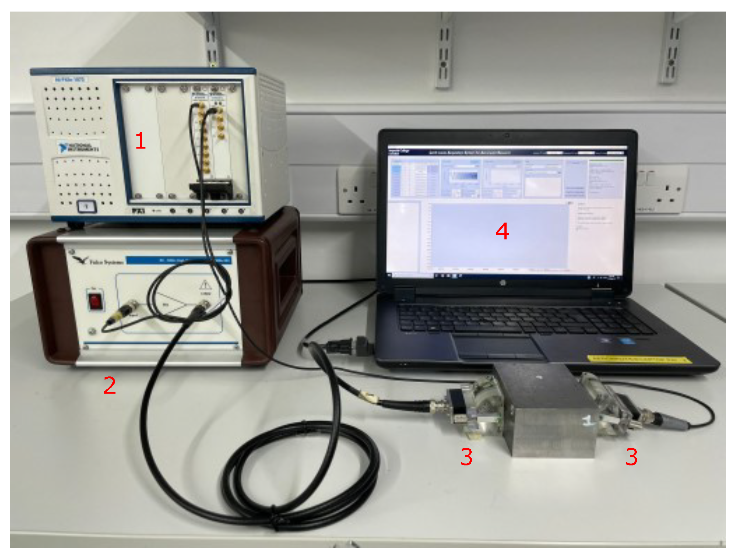
Figure 5 presents a schematic diagram that illustrates the essential components required for an experimental platform that is dedicated to damage detection applications using UGWs. The platform necessitates a minimum of five elements, namely a a signal generator (
in the figure), a power amplifier (
), an acquisition system (i.e., oscilloscope) (
), one or more transducers (
), and a personal computer (PC) (
). Specifically, the experimental step-by-step process from signal generation to acquisition was as follows:
The signal was generated with a NI-PXI wave generator;
The actuation signal was amplified using the amplifier module;
The resulting signal was applied by an Olympus A413S transducer to the specimen to initiate the desired response;
Another transducer, functioning as a sensor, was employed to capture the resulting signals;
The signal was acquired via an NI-PXI oscilloscope;
For data acquisition and manipulation, a PC equipped with dedicated acquisition software was utilized.
A 50 [mV] peak-to-peak amplitude, amplified 50 times by the amplifier with a center frequency of 500 [kHz], was applied with the actuation probe. The sampling frequency was set at 60 [MHz]. The total recording duration for the experimental signals was
s], and each measurement was recorded 50 times and averaged to enhance the signal-to-noise ratio. The transducer configuration employed was a pitch–catch arrangement, where the positions of the actuator and sensor were switched to account for the uncertainties based on the measurements, as depicted in
Figure 6.
The material under investigation was steel with the dimensions of
[mm],
[mm], and
[mm]. Moreover, the material properties assumed were
[GPa],
, and
[
38].
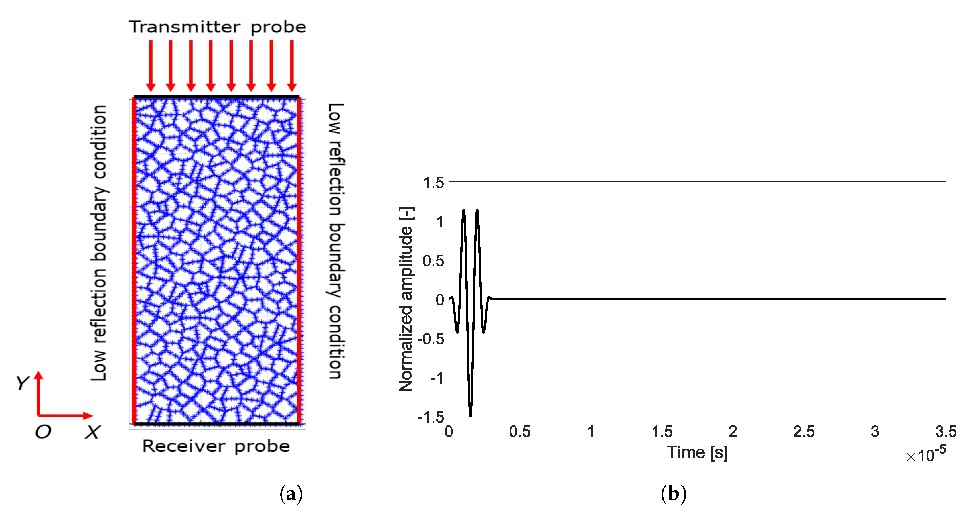
The micro-structure under investigation consisted of 100 randomly distributed grains with random material orientation. The average grain size was determined to be
[
39]. The 2D numerical model used had dimensions of
[mm
], as depicted in
Figure 7.
The input signal was defined at the upper edge of the micro-structure, where a prescribed traction of a 5-cycle tone burst with a Hanning window and center frequency of 500 [kHz] was enforced. The resulting signal was acquired at the bottom edge of the micro-structure. The time interval of the simulation was 25 [
s] with a time step of 10 [ns] and a time interval of the excitation of 10 [
s].
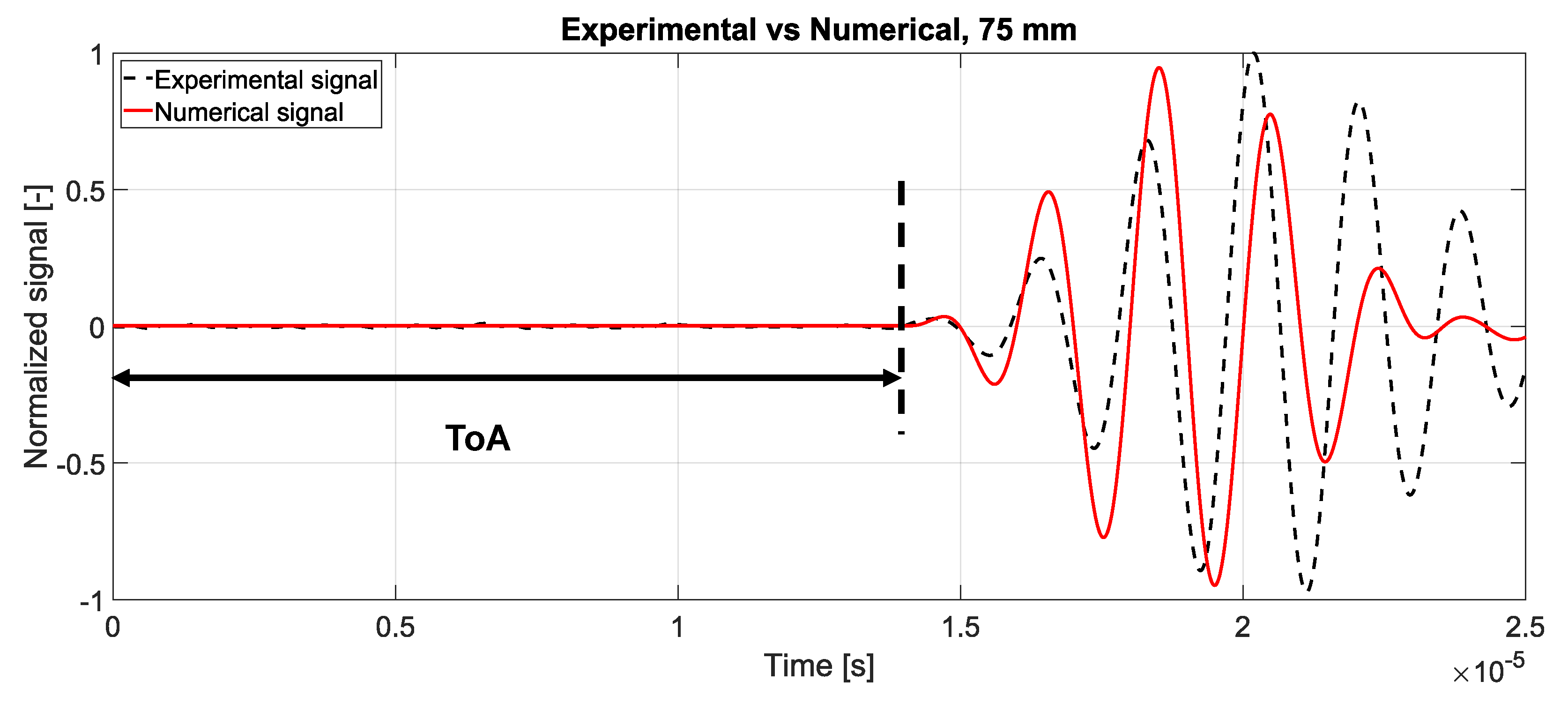
Figure 8 presents a comparative analysis of the experimental and numerical signals that were obtained from a sensor located at a distance of 75 [mm] from the actuator. The comparison revealed a strong agreement between the two sets of results in terms of ToA, amplitude, and wave velocity. Specifically, the experimental ToA value was measured at
s], while the corresponding numerical value was recorded as
s], thus resulting in a small relative error of
. The observed consistency between the experimental and numerical results indicated a reliable correspondence between the physical measurements and the numerical modeling. This agreement in ToA, amplitude, and wave velocity further validated the accuracy and effectiveness of the numerical simulation in capturing the behavior and characteristics of the system under investigation.
3.5. Missing Grains: Porosity
To investigate the impact of porosity on the macroscopic material properties, a parametric analysis was conducted by varying the number (#) of grains and the volume fraction of porosity [
47,
48,
49]. The analysis was performed under the assumption of a plain strain condition, and the material considered was aluminum. The dimensions of the micro-structure were 100 × 100 [mm
]. The specific details of the porosity model employed in this study can be found in the corresponding section of this paper. To assess the macroscopic properties, such as the elastic modulus (E) and shear modulus (G), the homogenization approach based on the RVE was utilized. The procedure for evaluating these properties is explained in detail in the dedicated section of this paper.
The volume fraction of porosity was calculated with Equation (
19).
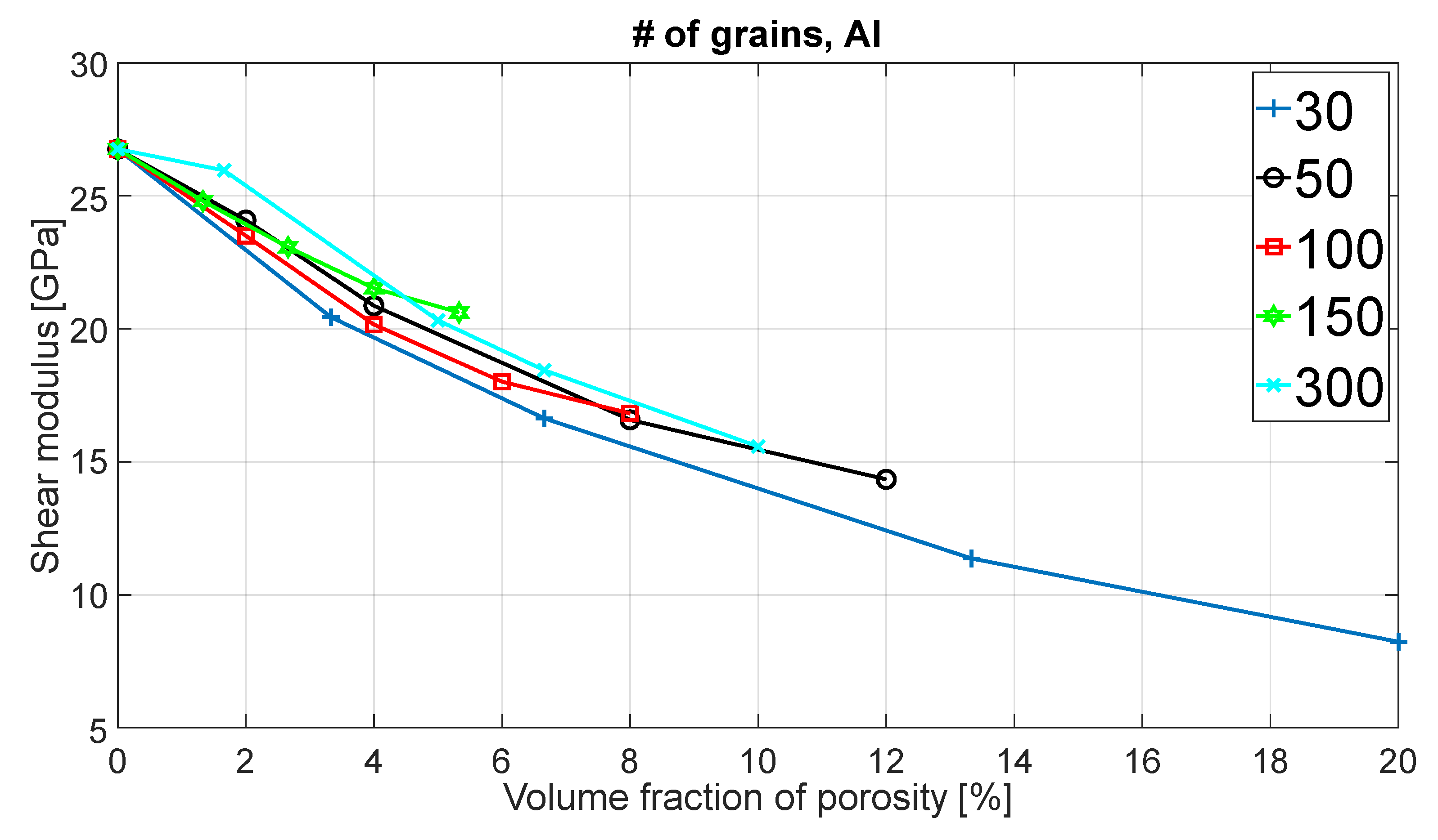
Figure 16 and
Figure 17 show the Young and Shear moduli, respectively, against the volume fraction of porosity, thus sweeping the number of grains from 30 up to 300. As expected, the higher the volume fraction of porosity, the lower the Young and Shear moduli.
To investigate the impact of porosity on grain morphology, three different materials with distinct grain shapes were tested: gold-silver (Ag-Si) with a rhombic crystal morphology, yttria (Y
2O
3) with a cubic crystal morphology, and alumina (Al
2O
3) with a truncated octahedral crystal morphology. The material properties for each of these materials are provided in
Table 1.
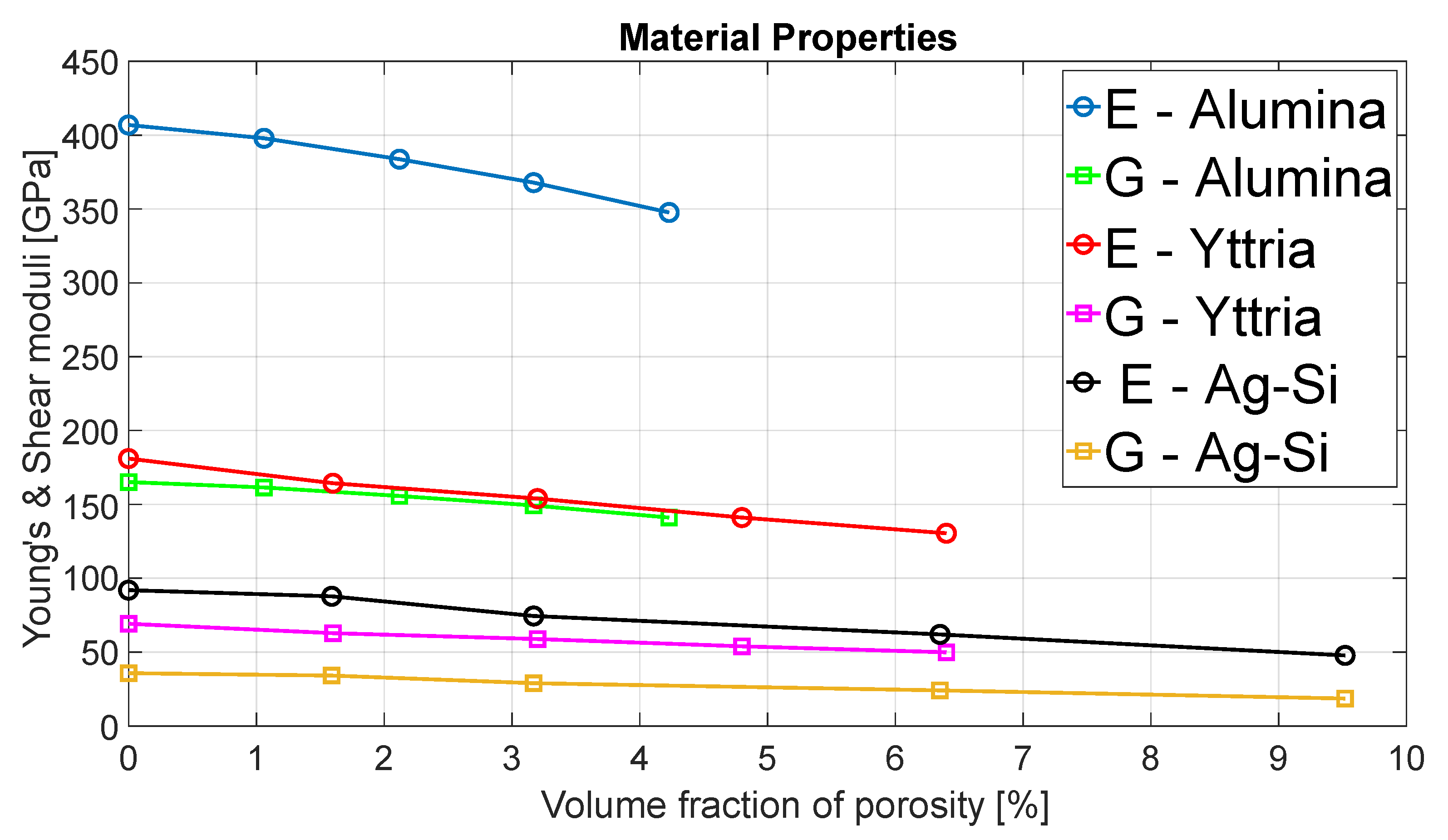
Figure 18 illustrates the variation of both the Young and Shear moduli against the volume fraction of porosity for alumina (189 grains), yttria (125 grains), and Ag-Si (63 grains). As expected, an increase in the volume fraction of porosity lead to a decrease in both the Young and Shear moduli for all three materials.
Furthermore, by analyzing the BEM results, it was possible to quantitatively evaluate the influence of the volume fraction of porosity on the macroscopic material properties.
Table 2,
Table 3 and
Table 4 present the volume fraction of porosity, Young’s modulus, Shear modulus, and the percentage difference of E and G compared to the pristine condition for all three materials. The analysis revealed that the volume fraction of porosity had a greater effect on E compared to G, particularly for the rhombic crystal morphology (Ag-Si), while the effect was less pronounced for both the cubic crystal morphology (yttria) and the truncated octahedral crystal morphology (alumina). To conclude the porosity analysis, simulations were performed to detect the presence of voids. The detection of voids was analyzed based on the changes in the amplitude and ToA of the backscattered signal. The simulations were performed with voids in different positions for an aluminum micro-structure. The input signal was defined at the upper edge of the micro-structure, where a prescribed traction 3-cycle tone burst with a Hanning window and center frequency of 1 [MHz] was enforced. The time interval of the simulation was 40 [
s] with a time step of 10 [ns] and a time interval of the excitation of 3 [
s]. The ToA was calculated from 0 to the starting point of the wave packet backscattered by the void itself. The starting point of the wave packet backscattered by the void itself was evaluated as the value of the wave above a threshold.
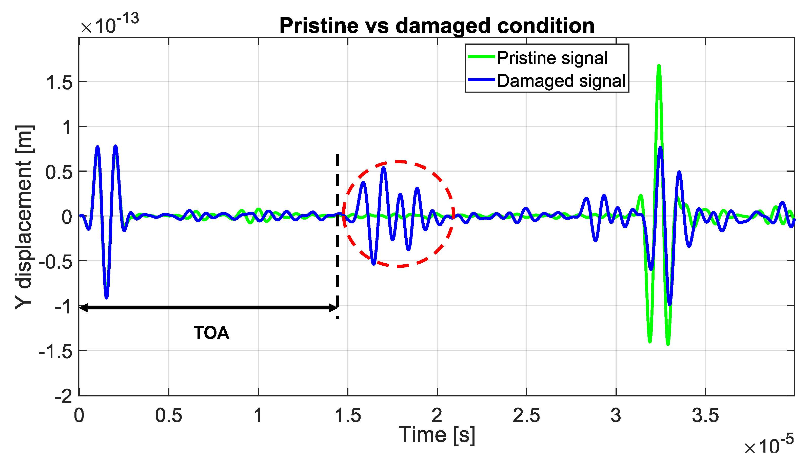
Figure 19 illustrates the comparison between the averaged Y displacement at the upper edge for the pristine and the damaged conditions for a 50-grain micro-structure. The damaged signal (depicted by the orange line in the figure) clearly exhibited the presence of a void, as indicated by the amplitude of a signal that was backscattered by the void itself (the dashed green circle indicates the part of the wave that was located in the wave that was backscattered by the void itself). Thus, the BEM model successfully detected the presence of the void.
Similarly,
Figure 20 presents the comparison between the averaged Y displacement at the upper edge for both the pristine and damaged conditions in 100-grain micro-structures. The damaged signal (represented by the blue line in the figure) revealed the presence of the void, which was confirmed by the amplitude of the signal that was backscattered by the void itself (the dashed red circle indicates the part of the wave that was located in the wave that was backscattered by the void itself). This demonstrated that the BEM model was capable of detecting the presence of voids that were located at different positions within the micro-structure.
3.7. Probability of Detection (PoD) with Inter-Granular Cracks
The Probability of Detection (PoD) curve method was extensively employed for evaluating the reliability of NDT techniques. The PoD represents the capability of an NDT method to detect a flaw of specific characteristics, such as type and size. PoD curves are constructed based on the characteristic dimensions of a certain defect, such as depth, length, orientation. These curves are influenced by various factors, including material properties, geometric features, defect types, operator skills, and environmental conditions [
55,
56]. Generating PoD curves typically requires a significant amount of experimental data, which can be expensive and time-consuming [
57,
58]. Consequently, there has been growing interest in utilizing simulation methods to reduce the reliance on extensive experimental testing. The concept of Model-Assisted and/or Simulation-Supported PoD has emerged in the past two decades, in which the aim is to leverage analytical or numerical models to enhance the efficiency and accuracy of PoD curve determination [
59,
60,
61]. Building upon the framework of Model-Assisted Probability of Detection (MAPoD), which has been utilized in numerous studies exploring simulation-based approaches to replace or supplement model-based approaches [
60,
61,
62], this research endeavors to investigate the feasibility of employing BEM simulations for generating PoD curves in the ultrasonic inspection of poly-crystalline micro-structures. To incorporate the influence of variability factors into the simulation, as well as to subsequently calculate the MAPoD, it is necessary to consider the potential sources of variability. For simplicity in this study, the sources of variability considered were the number of grains and grain morphologies, the material property variations, as well as crack length, crack orientation, and crack position. Specifically, the number of grains considered were 30, 50, and 100. For each number of grains, five different grains morphologies were considered, where the Young’s modulus varied within a range of 5% around the mean value for the corresponding material. The material under investigation was aluminum. The crack length was varied from
to 7 [mm], in increments of
[mm]. Both the location and orientation of the cracks were randomly distributed. Thus, 10 cracks located and orientated randomly for each crack length and for each grain morphology were considered, thereby resulting in a total of 50 combinations of variability sources per crack length. Consequently, a total of 700 simulations were conducted. Upon completion of all the simulations, the resulting scatter plot of the flaw responses was utilized to construct the PoD curve. The averaged vertical displacement at the upper edge was selected as the output signal. Snapshots from the BEM simulations that considered different scenarios are presented in
Figure 24,
Figure 25,
Figure 26,
Figure 27 and
Figure 28.
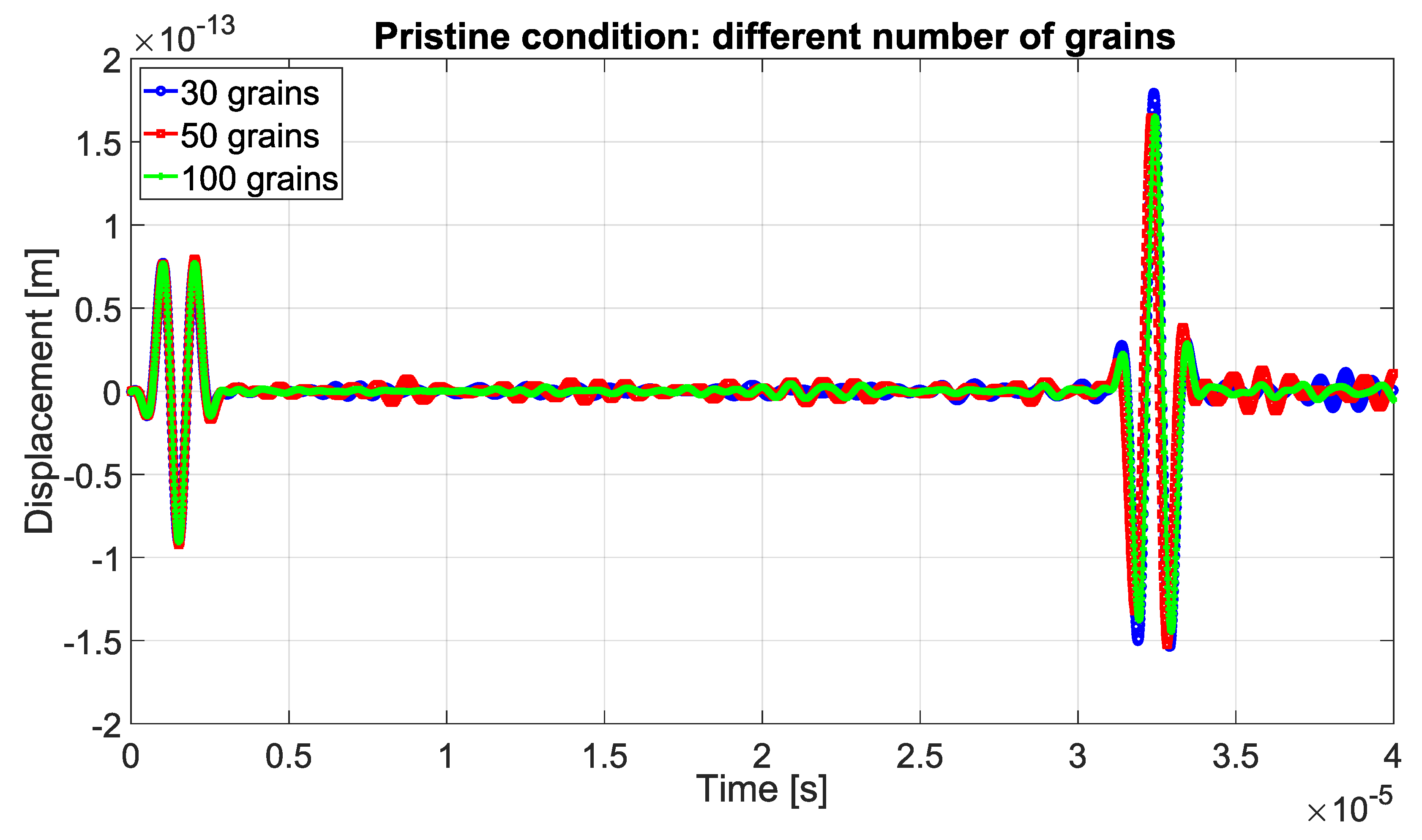
Figure 24 illustrates the averaged pristine signal obtained at the upper edge of the structure for varying numbers of grains, specifically 30, 50, and 100. As depicted in the figure, the signals exhibited excellent agreement in terms of both amplitude and the ToA.
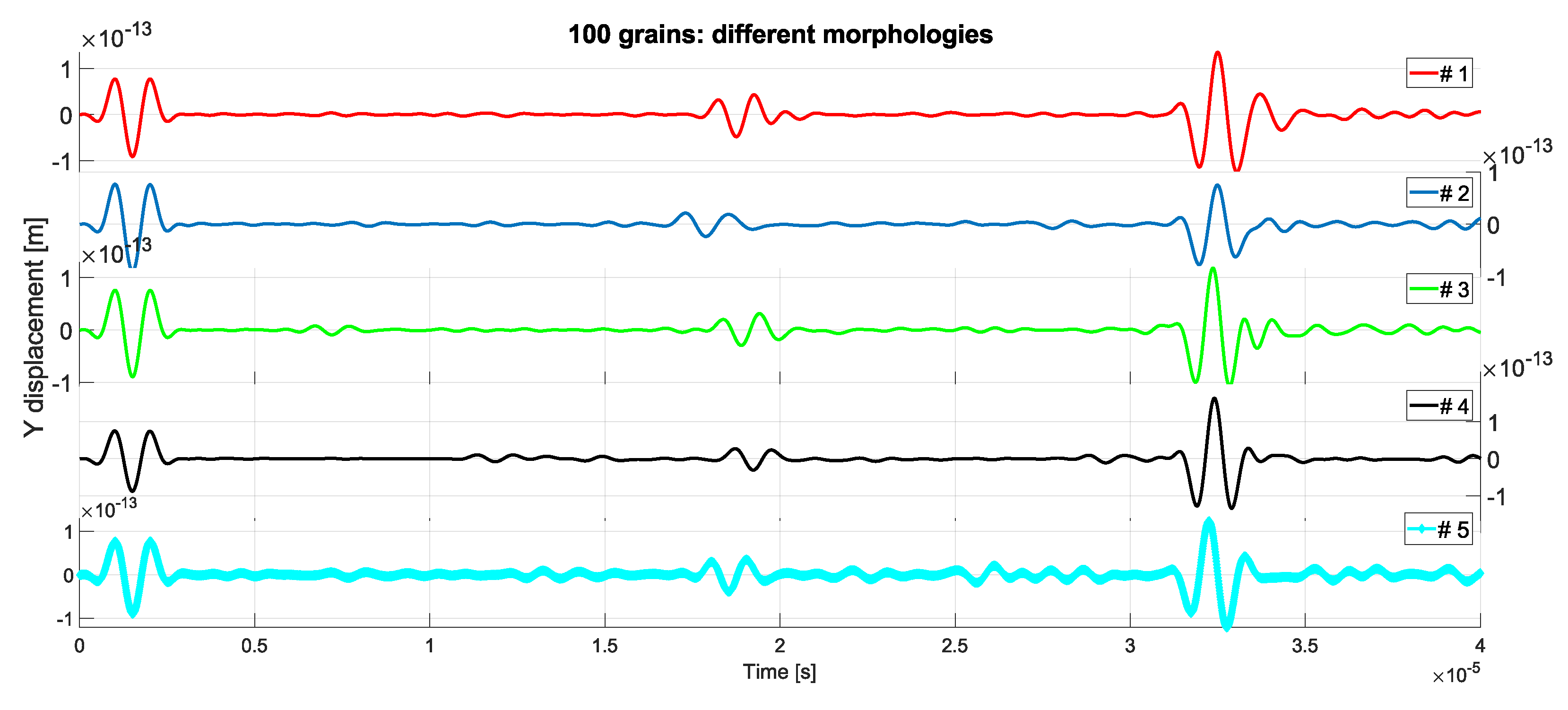
Figure 25 showcases a comparison of the signals generated from different grain morphologies while maintaining a fixed number of grains (i.e., 100 grains in this particular case). Notably, these five signals exhibited slight variations, particularly in terms of the ToA, because of the presence of distinct grain morphologies and their associated material properties.
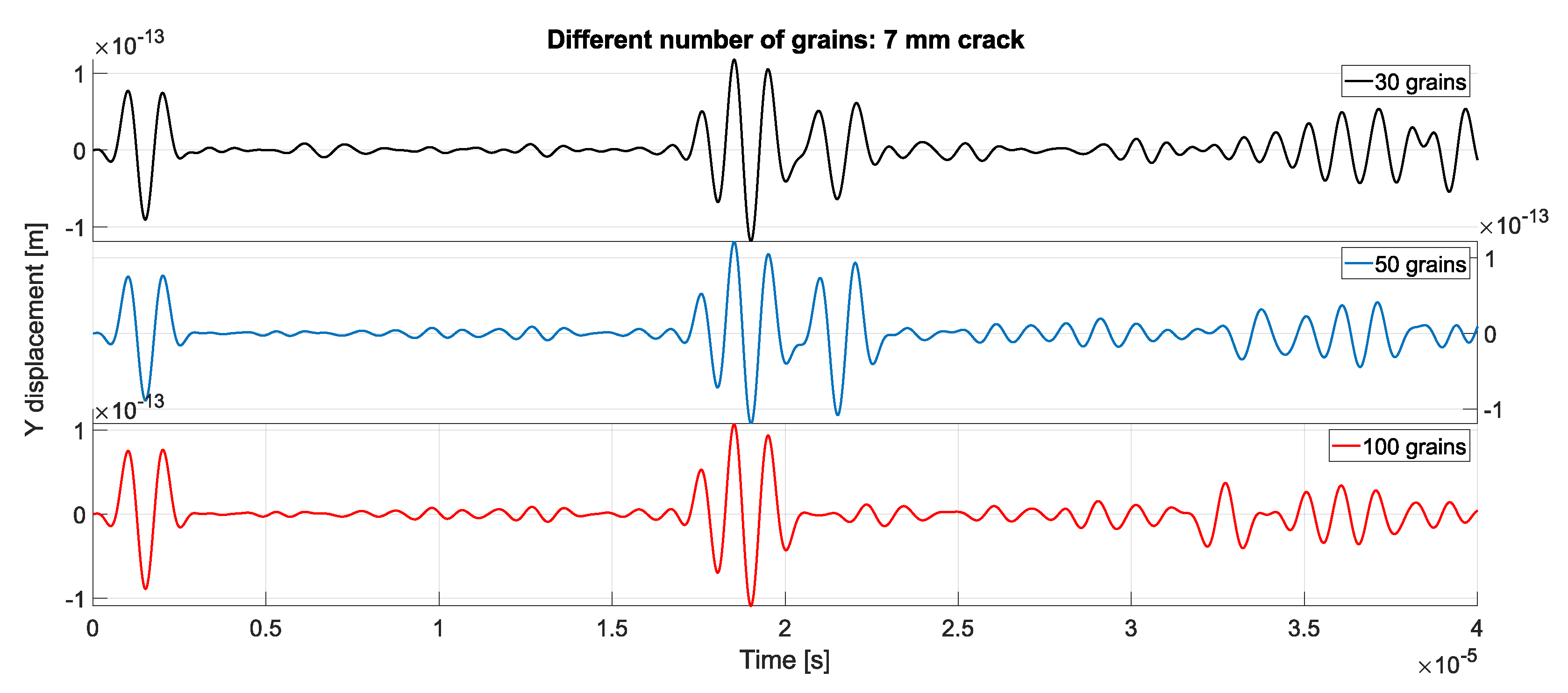
Figure 26 presents the signals obtained under the damaged condition, specifically with a 7 [mm] crack, for varying numbers of grains. As observed in the figure, there was a noticeable increase in the signal amplitude that originated from the crack as the crack length increased. Consequently, the amplitude of the backscattered signal from the upper edge decreased, thereby indicating that long cracks significantly impact the overall signal amplitude.
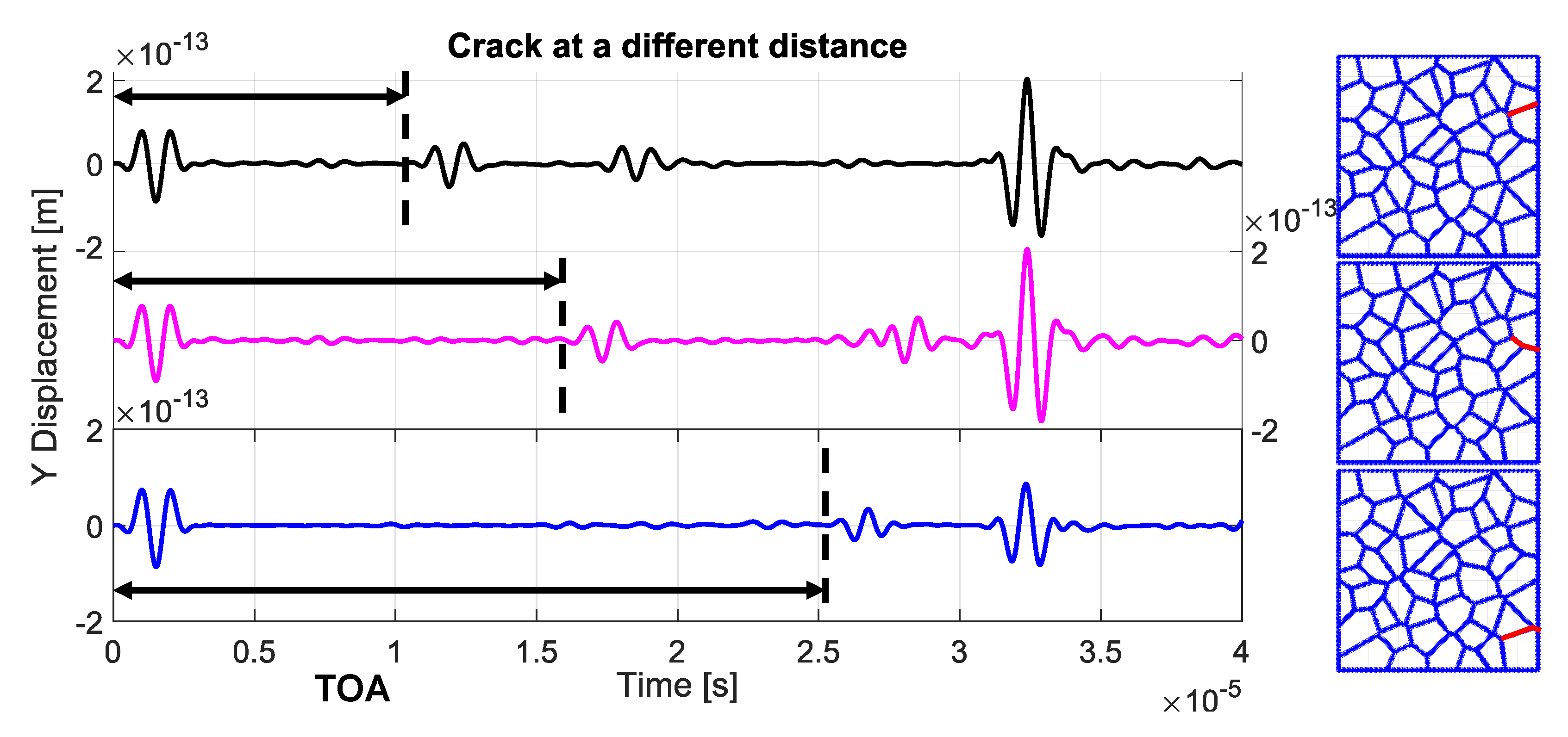
Figure 27 presents the signals obtained under the damaged condition with varying crack orientations, namely
,
, and
. Notably, the backscattered signal from the crack with a
orientation exhibited the highest amplitude, while the amplitude decreased as the crack angle increased. This behavior can be attributed to the fact that the wave is perpendicular to the
crack, thus resulting in maximum signal strength. Furthermore, the duration of the backscattered signal increased with an increasing crack angle. This is because of the decrease in signal amplitude, which requires more time for the same energy to be dissipated.
Figure 28 displays the signals obtained for a 2 [mm] crack length, in which different numbers of grains were considered. As depicted in the figure, the signals exhibited excellent agreement in both amplitude and the ToA.
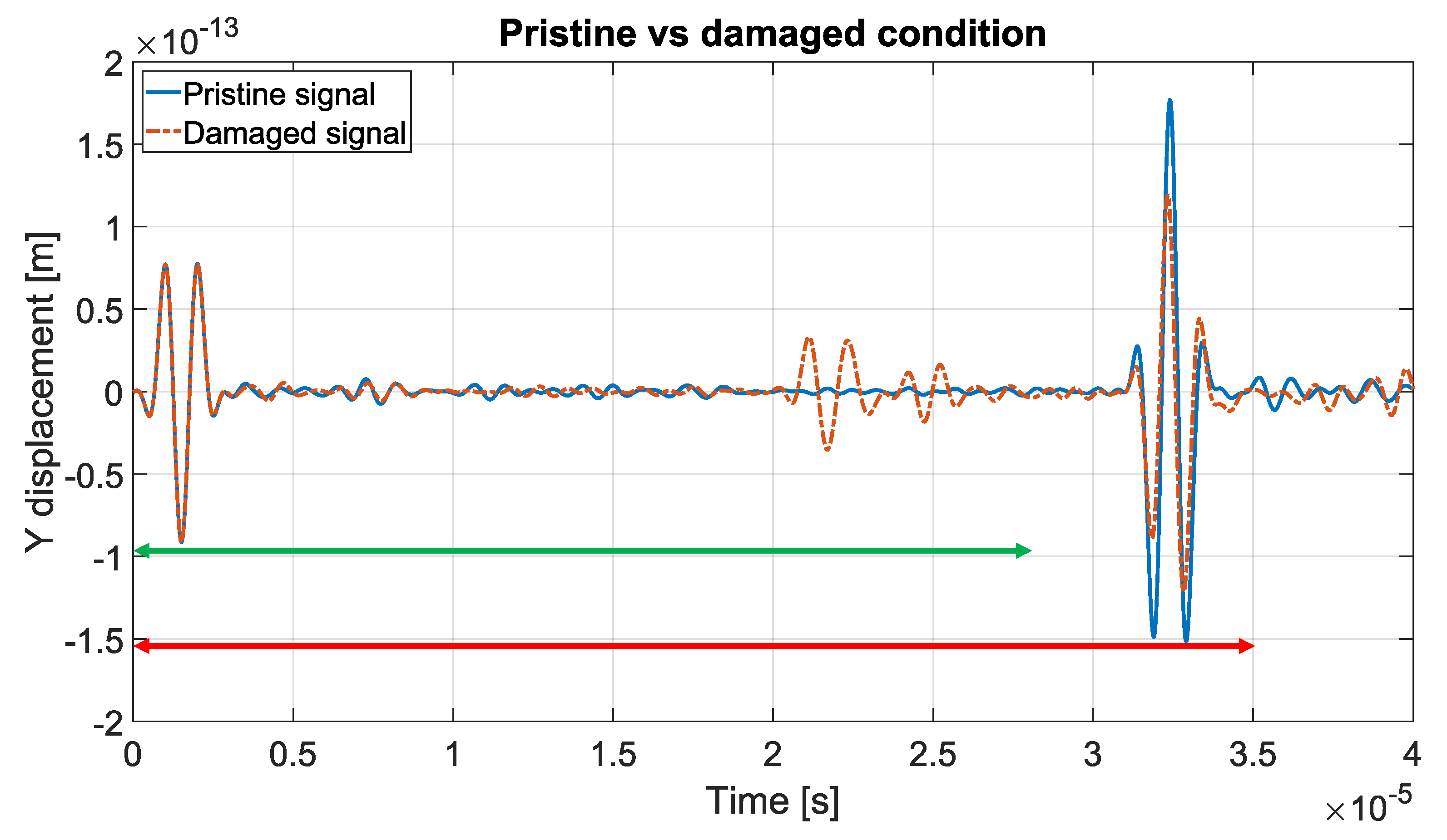
To eliminate the effect of multiple boundaries reflecting the signal, there were two choices to select with respect to the inspection interval (time window):
Up to the first back-wall reflection signal (time interval in red arrows in
Figure 29);
Up to the damaged backscattered signal (time interval in green arrows in
Figure 29).
In this study, the selected time interval of inspection was the first one and, in the case that the first wave packet was ambiguous and could not be clearly identified, the time window for the first wave packet was manually determined based on the signal characteristics.
Let
denote the damaged signal and let
denote the corresponding pristine state signal. The residual signal
, was obtained by subtracting the pristine signal from its damaged signal:
. Many existing approaches for damage detection involve extracting damage-sensitive features from UGW signals and establishing an index that indicates the presence of damage (commonly referred to as the Damage Index (DI)). The damage index was then compared to a threshold value, above which the presence of damage was signified. The damage detection strategy involved comparing the current signal with its baseline signal and quantifying the changes. In this case, the current signals were recorded under the same environmental and loading conditions, and any deviation from the baseline signal was attributed to the presence of damage. The magnitude of the deviation was quantified by the DI. The damage index used in this analysis was the reduction in correlation coefficient between the signal and its baseline, noted as
:
where
is the covariance of the signals and
is the standard deviation of the signals, respectively. This damage index takes into consideration both the difference in amplitude and in the ToA.
There are many ways to evaluate the threshold value. In this study, the threshold value was evaluated as follows:
The DI in the pristine state was evaluated with the following:
where
is the signal in a pristine state with a fixed actuation signal location and 1 [MHz] frequency, while
is the signal in a pristine state with uncertainties in both the actuation location and the frequency. As this procedure was followed for each morphology, five different DIs in pristine condition were obtained.
Figure 30 shows the DI in a pristine condition for the 100-grain case with a fixed morphology (i.e.,
). The DI exhibited a normal distribution, as illustrated by the black line on the right side of the plot. The dashed red lines refer to one standard deviation or
. The DI values ranged from 0.24 to 0.34, with a mean value of 0.29.
Figure 31 presents the DI in a damaged condition for the 100-grain case (morphology
), which was plotted against the crack length. As expected, the results clearly demonstrated that the DI increased with an increase in crack length. The dashed red line corresponds to the threshold value, while the dashed black line represents the mean value of the DI for each crack length.
There were two main approaches commonly employed to generate PoD curves, namely, hit/miss data and signal response analysis (“
” vs. “a”) [
60,
61]. The hit/miss approach provided binary results, indicating whether a flaw of a known size was detected or not. In this analysis, the number of detected cracks, “n”, was divided by the total number of simulated cracks, “N”, thereby yielding a reasonable assessment of the inspection system’s capability,
. This approach provided a single value representing the entire range of crack sizes. However, since larger cracks are typically easier to detect than smaller ones, cracks are often grouped based on their sizes, and
was calculated for each size range.
Figure 32 illustrates the PoD obtained using the hit/miss approach, which was plotted against the crack length. As depicted in the figure, the PoD increased as the crack length increased, reaching its maximum at a crack length of 5 [mm].
The second approach for determining the PoD was of much interest for several practical applications since it gave more information through the recorded defect response “
”, which was correlated with the defect characteristic dimension “a” [
60,
61,
63,
64]. This method utilizes regression analysis with Maximum Likelihood Estimation (MLE) to calculate the regression coefficients and their covariance matrix. From the variance of the expected regression response, confidence bounds at a
level can be constructed for “a”. To compute the PoD parameters, the threshold value was determined based on the consideration stated before. The variance (
) was utilized to estimate confidence intervals and the covariance matrix for PoD. The PoD could be generated for each crack by calculating the probability of the signal response when it exceeds the decision threshold value. In this analysis, the target variable was the crack length.
Figure 33 depicts the regression analysis for the 100-grain case, where the crack length is represented on the “
x” axis and the DI is displayed on the “
y” axis.
Figure 34 illustrates the PoD curve for the 100-grain case as a function of crack length. The important features of the model were recorded on the curve, including the
confidence interval (CI) area, as well as both the lower and upper bound of the PoD curve and the mean value. Furthermore, the
value, which is the
confidence bound on the
estimate, is displayed in the plot.
As depicted in
Figure 34, the PoD exhibits the expected behavior, where an increase in crack length corresponds to an increase in PoD. The PoD curves obtained from the BE simulations aligned with this expectation, thus demonstrating the potential of simulations for PoD characterization (particularly for crack lengths exceeding 3 [mm]). However, within the defect length range of 0–3 [mm], the PoD values were notably low. This discrepancy may be attributed to the limitations of the assumed parameters in the BEM simulations, which failed to accurately capture the intricacies associated with the smaller cracks in reality. Additionally, factors such as the noise sources that diminished the measured reflection amplitude, as well as the actual conditions of the wave generation and reception, needed to be incorporated into the simulations for a more comprehensive representation. Ongoing research aims to refine the representation and establish bounds for parameter uncertainties, which will contribute to enhanced predictions of PoD based on the BEM approach.
However, for defect lengths ranging from 0 to 3 [mm], a low PoD value was observed, possibly due to uncertainties in the assumed parameters not capturing the reality for smaller cracks. Incorporating finer details such as noise sources, which reduce the amplitude of measured reflection, and realistic wave generation and reception conditions into simulations is an ongoing effort to improve the accuracy of PoD predictions based on the BEM.


