A High-Precision Planar NURBS Interpolation System Based on Segmentation Method for Industrial Robot

Abstract

NURBS curve parameter interpolation is extensively employed in precision trajectory tasks for industrial robots due to its smoother performance compared to traditional linear or circular interpolation methods. The trajectory planning systems for industrial robots necessitate four essential functional modules: first, the spline curve discretization technique ensuring chord error compliance; second, the contour scanning technique for determining the maximum feasible feed rate for multi-constraint and multi-segment paths; third, the technique for achieving a smooth feed rate profile; and fourth, the continuous curve parameter interpolation technique. Therefore, this paper proposes a high-precision planar NURBS interpolation system for industrial robots. Firstly, a segmentation method for NURBS curves based on a closed-loop chord error constraint is proposed, which segments the original global NURBS curve into a collection of Bezier curves that strictly meet the chord error constraint. Secondly, a bidirectional scanning technique is presented to meet the joint space constraint, establishing an analytical mapping between the tool tip kinematic constraint and the joint kinematic constraint. Then, based on the traditional S-shaped feed rate profile, an adaptive algorithm with a displacement constraint is introduced, considering the real-time speed adjustment requirements of robots. Finally, a compensation interpolation strategy based on arc length parameterization is adopted to solve the accumulated error problem in parameter interpolation. The effectiveness of and potential for enhancing the quality of planar machining of the proposed planar NURBS interpolation system for industrial robots are validated through simulations and experiments. The results demonstrate the system’s applicability and accuracy, and its ability to improve planar machining quality.

1. Introduction

Industrial robot machining systems not only have weak stiffness characteristics compared to traditional numerical control (CNC) machining systems, but also have constraints on tool path chord error and nonlinear kinematic mapping issues. These are the main factors that affect machining quality and trajectory accuracy. The purpose of robot body control and compensation is to reduce the influence of joint weak stiffness on trajectories, while the purpose of industrial robot interpolation systems is to improve the accuracy and efficiency of trajectories. Therefore, the adjustment of the feed rate in the industrial robot curve parameter interpolation system plays a key role in the high-speed and high-precision machining of molds, aerospace parts, and other applications [1]. Smooth trajectories can help robots avoid sudden load changes, extend the life of joints, and improve position control accuracy. On the other hand, discontinuous feed rates can cause vibrations in the mechanical structure and servo control system, thereby reducing contour accuracy, affecting trajectory accuracy, and leading to task failures or even accidents [2]. Therefore, the research on high-precision trajectory planning and interpolation systems for industrial robots is of great significance. In order to achieve high-speed and high-precision machining, many scholars have devoted themselves to studying techniques such as parameter curve segmentation, feed speed contour adjustment, and parameter curve interpolation. Traditional flat paths typically use a large number of short line segments instead of the entire curve, which inevitably leads to discontinuous tangent directions and abrupt changes in curvature, resulting in a decrease in feed rate. Due to the lack of G1 and G2 continuity at the junctions of adjacent line segments, rate fluctuations and changes in acceleration often occur. Nonuniform rational B-spline (NURBS) parameter curves have effectively addressed the above problems [3] and have become the standard format for free-form curves and surfaces.

Based on the above issues, the current mainstream research content on planning and interpolation systems can be divided into three aspects. Firstly, there is the estimation method for NURBS path chord error. Currently, the majority of studies utilize curvature threshold segmentation techniques, which belong to open-loop chord error control and cannot ensure that real-time curve interpolation meets the chord error requirements throughout the entire machining process. Although there have been some studies [4,5,6] on accurately calculating chord error, the calculations are quite complex, so approximate estimation methods such as the second-order penetration circle method [7] are commonly used. Hua et al. [8] proposed a B-spline approximation scheme method with tool tip position adjustment. NURBS is divided into several subdivisions according to the discrete curvature. However, it requires iterative computation of new control points, which is inefficient and alters the original curve shape. Bi et al. [9] proposed a B-spline fitting scheme taking advantage of the B-spline’s strong convex hull property. In this process, the knot vectors and control points of curve segments, exceeding the prescribed tolerance for chord errors, are refined analytically. The optimization technique [10] fully utilized the tolerance band to minimize the maximum curvature of a B-spline curve with seven control points by adjusting the positions of two control points. However, this approach was specifically employed for local transitions. Ward et al. [11] proposed a novel approach for adaptively discretizing lengthy linear toolpaths to confine nonlinear interpolation errors. Nevertheless, the existing error models are not applicable to industrial robots. Recently, Shi et al. [12] constrained the nonlinear errors in the path in joint space, achieving motion smoothness. However, the drawback is that the errors in this approach cannot be analytically controlled. By using curvature scanning to obtain critical points on the curve and dividing the curve into multiple subcurves [13], it cannot be guaranteed that the chord error in the segmented curves satisfies the given constraints. Secondly, there is a need for real-time trajectory generation technology that calculates robot trajectories satisfying kinematic constraints for each axis. Known constraint parameters are required for feed rate scheduling. Ref. [14] proposes a relatively comprehensive S-shaped feed rate scheduling algorithm (CSFA) with restrictions on jerk, acceleration, and feed rate. It uses a dynamic forward–backward scanning strategy with restrictions on chord error, normal/tangential acceleration, jerk, and feed rate. However, in the error compensation part, a segmented rounding method is used. Although it eliminates the error in segmented arc length interpolation, it introduces feed rate fluctuations at adjacent spline connection points and does not consider robot joint constraint issues. Since the bidirectional scanning cannot guarantee the success of dynamic forward scheduling, ref. [15] introduces the feed rate bisection method to search for feasible boundary velocities. Although it can solve the problem of failed dynamic forward scheduling, its execution efficiency is severely reduced. To compensate for the limitations of unidirectional S-curves in NURBS curve feed rate scheduling applications, Liu et al. [16] proposed a bidirectional scanning algorithm that obtains feed rate parameters for key points and considers the rounding error and its compensation strategy to improve interpolation accuracy. However, this method does not consider the constraint of a contour error in the middle part of the curve segment, resulting in the speed exceeding limits in the planned curve.

To consider the continuous existence of constraints, it is essential to use smooth velocities for trajectory planning. Although the trapezoidal feed rate scheduling method is simple to implement [17], the discontinuity in acceleration can cause vibrations during frequent acceleration and deceleration, leading to a decrease in the lifespan of the motion equipment. The G1 and G2 discontinuities occurring at the junctions of two linear segments inevitably result in frequent feed rate fluctuations and acceleration variations [18]. Therefore, toolpath smoothing operations are crucial in numerical control systems to improve path continuity [19]. To address this problem, many feed rate scheduling methods that restrict acceleration jumps have been proposed, such as the time-optimal method [20,21], the sine-shaped method [22], and the S-shaped method [23,24]. Nguyen et al. [25] designed a systematic approach to design time-optimal S-curve motion profiles. Y. Bai et al. [26] studied the asymmetric motion properties of feed rate scheduling, as traditional or most feed rate planning methods rely on symmetric formulas for the start and stop segments, but the time is not optimized in those cases. Thirdly, for the parametric solution of NURBS curve interpolation, Shipitalni et al. [27] performed a first-order Taylor expansion treating the interpolation parameters as a function of time, but the calculation precision is not high. To improve the calculation precision, Yeh et al. [28] proposed an interpolation point parameter solution algorithm based on second-order Taylor expansion, but it requires a large amount of computation, which impacts the real-time capability of the algorithm. M. Tikhon [29] proposed that within each interpolation period, the maximum feed rate is determined by the specified chord error and constant material removal rate. In existing research [30,31], it has been demonstrated that the Taylor expansion method can generate trajectories identical to the reference method, but feed rate fluctuations are inevitable in regions with high curvature. An optimization algorithm [32] is proposed to improve the precision of NURBS curves. This algorithm employs an iterative process to calculate block displacement, with the NURBS parameter u as the optimization target. However, the requirement to repeatedly compute the accurate value of u results in the inability to perform online interpolation. Most interpolation methods use Taylor expansion to approximate the next interpolation parameter.

In response to the above issues, this article proposes a tool speed scheduling and high-precision interpolation system for industrial robots for NURBS curves. Firstly, a fast and accurate calculation method for tool path curvature is proposed. The knot insertion technique is introduced to segment the original tool path into segments based on curvature, which creates a set of rational Bezier curves. The entire processing curve is ensured to meet the requirements of the chord error. Secondly, considering the impact of the nonlinear kinematics of robot joints, a dynamic optimization of the maximum feed rate and maximum acceleration is conducted during the bidirectional scanning process of the traditional feed rate extrema curve. This optimization achieves dynamic speed regulation and braking functions within an adaptive S-shaped feed rate profile. The preset values for the maximum feed rate and maximum acceleration constraints in bidirectional feed rate scanning are adjusted, ensuring smooth robot interpolation while adhering to joint kinematic constraint. Finally, during the curve interpolation stage, a compensation interpolation strategy using Taylor expansion and arc length parameterization is applied to the segmented NURBS curve set. The parameter remapping method is used to ensure parameter continuity at the junction points of adjacent curve segments, without transferring all the original NURBS control points to the underlying structure. This reduces storage capacity and eliminates nonlinear errors in interpolation.

The remaining sections of the paper are organized as follows. Section 2 proposes a method for segmenting NURBS curves into a set of rational Bezier convex curves based on a closed-loop chord error constraint. Section 3 introduces an improved adaptive S-shaped feed rate scheduling algorithm, which achieves an adaptive planning mode under a given displacement. It also presents a method for robot speed control and braking planning under arbitrary states, enabling smooth speed regulation and braking based on S-shaped feed rate scheduling. Section 4 proposes a bidirectional feed rate profile scanning algorithm that effectively combines robot joint constraints to meet maximum performance requirements. Section 5 addresses the problem of the continuous interpolation of convex curve sets and presents a parameter remapping method based on Taylor expansion to ensure parameter continuity at the junction points of adjacent curves. Section 6 conducts NURBS processing tests on an industrial robot and provides experiments and simulations, and the conclusion is given in Section 7.

2. Segment NURBS into Bezier Curves Based on Closed-Loop Chord Error Constraint

2.1. Definition of NURBS Curve and Knot Insertion

This paper uses cubic NURBS curves to describe the planar machining path. The rational basis function representation of the NURBS curve equation is expressed as follows [3]:

$$\{\begin{array}{l}C(u)={\displaystyle \sum _{i=0}^n{P}_i{R}_{i,k}(u)}\\ R_{i,k}(u)=\frac{{\omega }_i{N}_{i,k}(u)}{{\displaystyle \sum _{j=0}^n{\omega }_i}{N}_{i,k}(u)}\end{array}$$

(1)

In the equation, the k-th rational basis function is denoted as R_i,k(u) and has properties similar to those of the k-th normalized B-spline basis function N_i,k(u), such as normality, local support, and differentiability. ${\omega }_i$ is the weight factor, and the control points are represented by P_i. Connecting them in order with line segments forms the control polygon.

$$\{\begin{array}{l}{N}_{i,0}(u)=\{\begin{array}{c}\begin{array}{cc}1,& u_i\le u\le u_{i+1}\end{array}\\ \begin{array}{cc}0,\hfill & otherwise\hfill \end{array}\end{array}\\ N_{i,k}(u)=\frac{u-u_i}{u_{i+k}-u_i}{N}_{i,k-1}(u)+\frac{u_{i+k+1}-u}{u_{i+k+1}-u_{i+1}}{N}_{i+1,k-1}(u)\\ i=0,1,\dots ,n\end{array}$$

(2)

The nonuniform knots vector U is given as follows:

$$U=\left[\underset{k+1}{\underbrace{0,0,\dots 0,}}{u}_{k+1},\dots ,u_{n-k-1},\underset{k+1}{\underbracket{1,1,\dots ,1}}\right]$$

(3)

Although the cubic NURBS curves described above can solve the issue of smoothness in the path, the currently adopted curvature-based speed limiting technology belongs to open-loop bow chord error control, which cannot guarantee real-time compliance with chord error requirements throughout the entire machining process. To address this issue, this paper proposes a closed-loop chord error control technology for planar NURBS curves to improve machining quality. Firstly, the knot insertion technique is used to segment the original NURBS curves based on curvature, dividing the curves into multiple segments of cubic rational Bezier curves. Then, the parameter points where the curvature is zero are solved for each curve segment, and a projection algorithm is used to project the curves onto the coordinate axes. The precise chord error is obtained by differentiating the analytic cubic rational Bezier formula and obtaining the extreme points.

In order to obtain an analytical set of segmented Bezier curves, it is necessary to introduce the technique of knot insertion, which is a crucial technique in the fundamental geometric properties of spline curves. When new knots are inserted into the knot vector interval of the original spline curve, the equality relationship between the number of control points and knot s results in an increase in the corresponding number of new control points. Therefore, the node insertion technique achieves the following. Modification of Local Properties: By inserting nodes, the local properties of the original spline can be altered, allowing for the control of local shapes and enhancing local characteristics. This, in turn, increases the flexibility of the spline; and Generation of Local Beziers: When inserted knots generate new control points according to a certain rule, the original spline can be constructed into new local Beziers without altering the shape of the original spline. This property is advantageous for locally segmenting the spline into Bezier segments, making the control of segmented Bezier curves simpler, more convenient, and more efficient.

Therefore, the introduction of node insertion technology not only enhances the local characteristics of the original spline but also facilitates the segmentation and control of the spline, leading to improved efficiency. This paper leverages the characteristics of node insertion to generate additional control points. When new knots are inserted into the node vector interval of the original spline curve, the equation relationship between the number of control points and the number of nodes leads to an increase in the corresponding number of new control points. This paper takes advantage of the knot insertion technique to achieve the segmented rational Bezier subdivision of a NURBS curve. Assuming the knot vector of the original spline of order k with n control points is ${U=[u}_0{,u}_1,\dots u_{n+k+1}]$, and $u\in {[u}_i{,u}_{i+1}]$ is the knot to be inserted, then the new node vector is ${U=[u}_0{,u}_1,\dots {,u}_i{,u,u}_{i+1},\dots u_{n+k+1}]$, which can be rewritten as ${\overline{U}=[\overline{u}}_0{,\overline{u}}_1,\dots {,\overline{u}}_i{,\overline{u}}_{i+1},\dots {\overline{u}}_{n+k+2}]$. The new knot vector determines a set of new spline basis functions. In 1980, Boehm [33] introduced a method for calculating additional control points without changing the shape and parameters of the spline curve under the condition of knot insertion.

$${\overline{P}}_j=P_j,j=0,1,\dots ,i-k$$

(4)

$${\overline{P}}_j={\alpha }_j{P}_j+\left(1-{\alpha }_j\right)P_j, j=i-k+1,\dots ,i-r$$

(5)

$${\overline{P}}_j=P_{j-1}, j=i-r+1,\dots ,n+1$$

(6)

$${\alpha }_j=\frac{t-t_j}{t_{j+k}-t_j}, \left(\frac{0}{0}=0\right)$$

(7)

By using the knot insertion technique, a NURBS curve is segmented into multiple segments of Bezier curves. The rational fraction of a cubic Bezier curve can be simplified to the form of a polynomial numerator and denominator:

$$B\left(u\right)=\left(\frac{1}{w\left(u\right)}\right)\left[\left(1-u^3\right){\omega }_0{P}_0+3u{\left(1-u\right)}^2{\omega }_1{P}_1+3u^2\left(1-u\right){\omega }_2{P}_2+u^3{\omega }_3{P}_3\right],0\le u\le 1$$

(8)

$$w\left(u\right)={\left(1-u\right)}^3{\omega }_0+3u{\left(1-u\right)}^2{\omega }_1+3u^2\left(1-u\right){\omega }_2+u^3{\omega }_3$$

(9)

By using the knot insertion method, new control points and node vectors are created for NURBS by segmenting the NURBS curve into several Bezier curves.

Table 1. Bezier control points and node vectors obtained after the initial segmentation.

Curve Types	Control Points $\mathbf{\left[}\begin{array}{c}\mathit{x}\\ \mathit{y}\end{array}\mathbf{\right]}$	Node Vectors
NURBS	$\left[\begin{array}{c}\begin{array}{cccc}5& 6& 11& \begin{array}{ccc}8& 12& 11\end{array}\end{array}\\ \begin{array}{cccc}4& 12& 10& \begin{array}{ccc}4& 3& 9\end{array}\end{array}\end{array}\right]$	$\left[\begin{array}{ccc}0& 0& \begin{array}{cccc}0& 0& 1/3& \begin{array}{cccc}2/3& 1& 1& \begin{array}{cc}1& 1\end{array}\end{array}\end{array}\end{array}\right]$
Bezier 1	$\left[\begin{array}{cc}5& \begin{array}{cc}6& \begin{array}{cc}8.5& 9.25\end{array}\end{array}\\ 4& \begin{array}{cc}12& \begin{array}{cc}12& 9.5\end{array}\end{array}\end{array}\right]$	$\left[\begin{array}{cccc}0& 0& 0& \begin{array}{cccc}\begin{array}{cc}0& 1\end{array}& 1& 1& 1\end{array}\end{array}\right]$
Bezier 2	$\left[\begin{array}{cc}9.25& \begin{array}{cc}10& \begin{array}{cc}9& 9.5\end{array}\end{array}\\ 9.5& \begin{array}{cc}8& \begin{array}{cc}6& 4.75\end{array}\end{array}\end{array}\right]$	$\left[\begin{array}{cccc}0& 0& 0& \begin{array}{cccc}\begin{array}{cc}0& 1\end{array}& 1& 1& 1\end{array}\end{array}\right]$
Bezier 3	$\left[\begin{array}{cc}9.5& \begin{array}{cc}10& \begin{array}{cc}12& 11\end{array}\end{array}\\ 4.75& \begin{array}{cc}3.5& \begin{array}{cc}3& 9\end{array}\end{array}\end{array}\right]$	$\left[\begin{array}{cccc}0& 0& 0& \begin{array}{cccc}\begin{array}{cc}0& 1\end{array}& 1& 1& 1\end{array}\end{array}\right]$

includes the NURBS control points and knot vectors assigned in this study, and the results of the initial segmentation can be found in Figure 1.

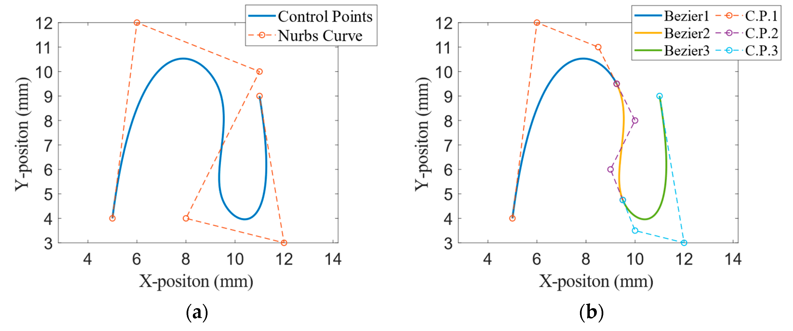
2.2. Curve Segment Based on Closed-Loop Chord Error

Although the knot insertion method can transform a NURBS curve into multiple Bezier curves by inserting new control points without altering the geometric type of the curve, the subdivided cubic Bezier curves have two types: C and S. Figure 1b shows the insertion results, where Bezier1 and Bezier3 are in type-C, and Bezier2 is in type-S. For type-C, there is only one extremum point, while type-S has two extremum points. The curve can be split into two type-Cs at the point where the curvature is zero. One simple method to solve this is by projecting the curve parameter u onto the x-axis, in which case the y-axis represents the distance from the curve to the line, which is the chord error. The curvature is defined as:

$$\kappa =\frac{\Vert \dot{B}(u)\times \ddot{B}(u)\Vert }{{\Vert \dot{B}(u)\Vert }^3}$$

(10)

where $\dot{B}(u)$ and $\ddot{B}\left(u\right)$ are the first and second derivatives of the curve, respectively, and the knot with zero curvature is obtained through Equation (10). Figure 2 shows the segmentation results.

Finally, according to the set chord error $\delta$, the new Bezier curves are continuously segmented into halves until the chord error of all Bezier curves meet the requirement. Figure 3 shows the second segmentation and subsequent iterative segmentation results. Details can be found in Algorithm 1.

The pseudo-code is proposed as follows to generate the chord error control method:

Algorithm 1: Segmentation of NURBS curve with chord error δc.
Input:	Input NURBS curve parameters, Chord error δ
Output:	Bezier curves that satisfy the δc
1:	knot insertion → Bezier curve Bi;
2:	for i = 1 to Bezier curve number do
3:	calculate the parameter u with zero curvature in the type-S curve Bi.
4:	calculate the δmax in the type-C curve Bi.
5:	If  δmax > δc then
6:	Bisection method → segment curve Bi → 1 Bi, 2Bi;
7:	do algorithm 1 for 1Bi;
8:	do algorithm 1 for 2Bi;
9:	else
10:	return 1Bi, 2Bi;
11:	end
12:	end

3. S-Shaped Feed Rate Profile Generation and Dynamic Speed Adjustment

3.1. S-Shaped Feed Rate Profile

In this section, we introduce the double S-shaped feed rate profile briefly. The S-shaped ACC/DEC profile, which consists of seven phases (T1, T2, T3, T4, T5, T6, T7), is shown in Figure 4.

The parameters include: v_s representing the initial feed rate, v_spe representing the operating feed rate, v_e representing the final feed rate, S representing the specified displacement, V_max representing the maximum feed rate (set to v_spe), A_max representing the maximum acceleration, and J representing the maximum jerk. t_s is defined as the variable time, t_ls is the critical time for acceleration and deceleration, and t_sp represents the duration of constant acceleration during the variable acceleration phase. The corresponding acceleration a(t), feed rate v(t), and displacement S(t) can be calculated based on time and the three acceleration states using the following formulas:

$$a(t)=\{\begin{array}{l}\mathrm{sign}\left(v_e-v_s\right)Jt,0\le t\le \frac{t_s-t_{sp}}{2}\hfill \\ \frac{1}{2}\mathrm{sign}\left(v_e-v_s\right)J\left(t_s-t_{sp}\right),\frac{t_r-t_{sp}}{2}<t\le \frac{t_s+t_{sp}}{2}\hfill \\ \mathrm{sign}\left(v_e-v_s\right)J\left(t_s-t\right),\frac{t_s+t_{sp}}{2}<t\le t_s\hfill \end{array}$$

(11)

$$v(t)=\{\begin{array}{l}{v}_s+\frac{1}{2}\mathrm{sign}\left(v_e-v_s\right)J{t}^2,0\le t\le \frac{t_s-t_{sp}}{2}\hfill \\ v_s+\frac{1}{8}\mathrm{sign}\left(v_e-v_s\right)J{t}_{ls}^2\hfill \\ +\frac{1}{2}\mathrm{sign}\left(v_e-v_s\right)J{t}_{ls}\left(t-\frac{t_{ls}}{2}\right),\frac{t_s-t_{sp}}{2}<t\le \frac{t_s+t_{sp}}{2}\hfill \\ v_s+\frac{1}{4}\mathrm{sign}\left(v_e-v_s\right)J{t}_{ls}^2\hfill \\ +\frac{1}{2}\mathrm{sign}\left(v_e-v_s\right)J{t}_{ls}{t}_{sp}-\frac{1}{2}\mathrm{sign}\left(v_e-v_s\right)J{\left(t_s-t\right)}^2,\frac{t_s+t_{sp}}{2}<t\le t_s\hfill \end{array}$$

(12)

$$S(t)=\{\begin{array}{l}{v}_{s}t+\frac{1}{6}\mathrm{sign}\left(v_e-v_s\right)J{t}^3,0\le t\le \frac{t_s-t_{sp}}{2}\hfill \\ v_{s}t+\frac{1}{48}\mathrm{sign}\left(v_e-v_s\right)J{t}_{ls}^3+\frac{1}{8}\mathrm{sign}\left(v_e-v_s\right)J{t}_{ls}^2\left(t-\frac{t_{ls}}{2}\right)\hfill \\ +\frac{1}{4}\mathrm{sign}\left(v_e-v_s\right)J{t}_{ls}{\left(t-\frac{t_{ls}}{2}\right)}^2,\frac{t_s-t_{sp}}{2}<t\le \frac{t_s+t_{sp}}{2}\hfill \\ v_{s}t+\frac{1}{4}\mathrm{sign}\left(v_e-v_s\right)J\left(-\frac{1}{2}{t}_{ls}^3-\frac{3}{2}{t}_{ls}^2{t}_{sp}-t_{sp}^2{t}_{ls}+t_{ls}^{2}t+2t_{ls}{t}_{sp}t\right)\hfill \\ +\frac{1}{6}\mathrm{sign}\left(v_e-v_s\right)J{\left(t_s-t\right)}^3,\frac{t_s+t_{sp}}{2}<t\le t_s\hfill \end{array}$$

(13)

The implementation process is as follows:

Step 1: Based on the input motion parameters and the relationship between v_s, v_e, and v_spe, determine if there is constant linear interpolation. If v_s, v_e, and v_spe are equal, it indicates that only constant linear interpolation exists in this planning, so proceed to interpolation with only the constant linear segment d. If the trajectory does not involve constant linear interpolation, proceed to step 2;

Step 2: According to the relevant formulas mentioned above, calculate the sum of displacements from v_s to v_spe, and v_spe to v_e, denoted as S₁. Calculate the variable displacement S₂ when directly accelerating from v_s to v_e, without going through v_spe;

Step 3: Based on the parameter relationships described above, perform classification and judgment, as shown in the flowchart in Figure 5.

3.2. Dynamic Speed Control Planning

Since this paper is based on the simplification of the problem with zero initial and final accelerations, the S-shaped method cannot achieve real-time transitions from any motion state to another. Therefore, this paper proposes a dynamic speed control planning that ensures speed changes and an acceleration reset in the shortest possible time within the original S-shaped feed rate profile framework.

First, when the initial acceleration is not zero and acceleration replanning is required, the maximum jerk J needs to be applied in order to make the acceleration become zero. By planning with the maximum jerk, we can calculate the time t_a0 and the corresponding velocity v_a0 needed to change the initial acceleration a_s to zero.

$$t_{a0}=\left|\frac{a_s}{J}\right|$$

(14)

$$v_{a0}=v_s+a_s{t}_{a0}+\frac{J{t}_{a0}^2}{2}$$

(15)

The formulas for interpolating position, feed rate, and acceleration based on jerk are as follows:

$$\{\begin{array}{l}S(t)=S(0)+(v_s+(\frac{a_s}{2}+\frac{Jt}{6})t)t\\ v(t)=v_s+(a_s+\frac{Jt}{2})t\\ a(t)=a_s+Jt\end{array}$$

(16)

At this point, the acceleration is reduced to zero, but there is still a nonzero feed rate. In the second step, it is necessary to replan the acceleration to ensure that the feed rate changes to the desired state with acceleration also being zero.

$$S_a(v_s,v_e)=\{\begin{array}{l}(v_s+v_e)\sqrt{\frac{v_e-v_s}{J_{\max }}}\hspace{1em}\hspace{1em}{v}_e-v_s\le \frac{A_{\max }{}^2}{J_{\max }}\\ \frac{1}{2}(v_s+v_e)\left[\frac{A_{\max }}{J_{\max }}+\frac{(v_e-v_s)}{A_{\max }}\right]\hspace{1em}\hspace{1em}{v}_e-v_s>\frac{A_{\max }{}^2}{J_{\max }}\end{array}$$

(17)

$$S_d(v_s,v_e)=\{\begin{array}{l}(v_s+v_e)\sqrt{\frac{v_s-v_e}{J_{\max }}}\hspace{1em}\hspace{1em}{v}_s-v_e\le \frac{A_{\max }{}^2}{J_{\max }}\\ \frac{1}{2}(v_s+v_e)\left[\frac{A_{\max }}{J_{\max }}+\frac{(v_s-v_e)}{A_{\max }}\right]\hspace{1em}\hspace{1em}{v}_s-v_e>\frac{A_{\max }{}^2}{J_{\max }}\end{array}$$

(18)

In the formula, A_max represents the maximum acceleration, and J_max represents the maximum jerk. Based on the current v_s and the desired v_e, a determination is made whether to accelerate or decelerate. If acceleration is required, Equation (17) is employed. Conversely, if deceleration is needed, Equation (18) is used. S_a and S_d denote the displacement for acceleration and deceleration, respectively. By ensuring an adequate length of displacement for feed rate lookahead, smooth braking can be achieved. Figure 6 illustrates these two scenarios.

4. Bidirectional Feed Rate Scanning of S-Shaped Profile

For the processing trajectory of the end effector of the manipulator, its feed rate vector is obtained by combining the tangential velocities of the tool tip and the tool axis direction, with its magnitude equal to the feed rate modulus and its direction determined by the tangential composition of the tool tip spline and the tool axis direction spline. In this study, the feed rate in the tool axis direction is set to zero. Similarly, the acceleration vector is obtained by combining the tangential acceleration and the normal acceleration of the tool tip and the tool axis motion. Therefore, the feed rate vector V and the acceleration vector A at any point on the processing trajectory of the manipulator‘s end effector can be expressed as follows:

$$\mathit{V}=\left[v\mathit{\tau },0\right]$$

(19)

$$\mathit{A}=\left[a\mathit{\tau }+\frac{v^2}{\rho }\mathit{n},0\right]$$

(20)

where the unit tangential at any point on the tool tip spline is denoted as $\tau$, while the unit normal at any point on the tool tip spline is denoted as $n$. The curvature radius is represented by $\rho$.

The obtained representation pertains to the feed rate and acceleration of arbitrary points on the processing trajectory in the task space. However, during the actual machining process, the known variables are the velocity $\dot{\theta }$ and acceleration $\ddot{\theta }$ constraints of each axis in the joint space. It becomes necessary to make real-time adjustments to the maximum feed rate and acceleration in the bidirectional velocity scanning, as well as the velocity extremum at the endpoints, based on the known kinematic constraints in the joint space. According to the differential kinematic relationship, the following mapping relationships exist between the velocity and acceleration vectors in the joint space and the task space.

$$\dot{\mathit{\theta }}={\mathit{J}}_{ac}{}^{-1}\mathit{V}$$

(21)

$$\ddot{\mathit{\theta }}={\mathit{J}}_{ac}{}^{-1}\mathit{A}-{\mathit{J}}_{ac}{}^{-1}{\dot{\mathit{J}}}_{ac}\left({\mathit{J}}_{ac}{}^{-1}\mathit{V}\right)$$

(22)

The feed rate constraints in the bidirectional scanning can be divided into geometric constraints and time constraints in the task space. Geometric constraints include the maximum feed rate $V_{\max }$, maximum normal acceleration $A_{n,\max }$, and maximum normal jerk $J_{n,\max }$. Time constraints consist of the maximum tangential acceleration $A_{t,\max }$ and maximum tangential jerk $J_{t,\max }$. The geometric parameters of the path include the maximum chord error $\delta$ and the curvature ${\kappa }_{i,\max }$ at key points along the curve segment. These parameters summarizing the tangential velocity constraints in the task space are discussed in Reference [9]. In this paper, we provide a summary in the bidirectional scanning flowchart as shown in Figure 7. In the figure, the velocity curve from right to left represents the backward scanning, and vice versa for the forward scanning.

In order to simplify calculations, it is common to approximate the feed rate at points along the path as the maximum or very close to the maximum velocity. Based on this approximation, the formulas for correcting the maximum tangential feed rate and acceleration are straightforward. By calculating the corresponding Jacobian matrix J_ac and the curve unit tangent $\tau$, optimized values for the maximum tangential feed rate $V_{\max }^{\mathrm{opt}}$ and maximum tangential acceleration $A_{\max }^{\mathrm{opt}}$ can be obtained. The formulas are as follows:

$${\mathit{V}}_{\max }^{opt}=\min \left({\mathit{V}}_{\max },\frac{{\dot{\mathit{\theta }}}_{\max }}{{\mathit{J}}_{ac}{}^{-1}\mathit{\tau }}\right)$$

(23)

$$A_{\max }^{opt}=\min \left(A_{t,\max },\frac{{\ddot{\theta }}_{\max }+J^{-1}\dot{J}\left(J^{-1}V\right)}{J^{-1}\mathit{\tau }}\right)$$

(24)

Assuming the current iteration is the i-th segment, with a lookahead window length of N, the end feed rate of the (i − 1)th segment (the start feed rate of the i-th segment) is denoted as $V_{\mathrm{end},i-1}$. The lookahead sublist of segment length is represented as $L_{i,\mathrm{list}}^{\left(N\right)}{=\text{{}L}_0{,L}_1,\cdots {,L}_i,\cdots {,L}_N\text{}}$, and the lookahead sublist of feed rates is denoted as $F_{i,\mathrm{list}}^{\left(N\right)}{=\text{{}F}_0{,F}_1,\cdots {,F}_i,\cdots {,F}_N\text{}}$. Additionally, the forward scanning feed rate is calculated as $V_{\mathrm{end},i}^f$ and the backward scanning feed rate as $V_{\mathrm{end},i}^b$. Considering all velocity constraints and optimization strategies, the dynamic lookahead bidirectional scanning algorithm follows the workflow outlined Algorithm 2 below:

Algorithm 2: Bidirectional Scanning.
Input:	$V_{end,i-1}$ is the end feed rate of the (i − 1)th segment (the start feed rate of the i-th segment); $L_{i,list}^{\left(N\right)}$ is the lookahead sublist of segment length; $F_{i,list}^{\left(N\right)}$ is the lookahead sublist of feed rates; Vmax is the maximum feed rate; At,max/Jt,max are the maximum tangential acceleration/jerk; $\delta$ is the maximum chord error; ${\kappa }_{i,max}$ is the curvature at key points along the curve segment; An,max/Jn,max are the maximum normal acceleration/jerk; Ts is the sampling period.
Output:	Vend,i
Step 1:	1.1. If N = 1, stop the lookahead calculation and let Vend,i = 0; Otherwise, go to 1.2.
	1.2. Let k = N − 1, $V_{end,i}^b$ = 0;
Step 2:	2.1. $L_{i,list}^{\left(N\right)}$[0], Vend,i−1, $F_{i,list}^{\left(N\right)}$[0], Jt,max, At,max, Ts are utilized in the backward scanning, recursively backtracking from the last segment of the lookahead window to the second segment, to calculate the end feed rate $V_{end,i}^b$ based on the current segment velocity and constraints;
	2.2. The minimum feed rate under the given geometric constraints, as well as the kinematic constraints in both the task space and joint space, is assigned as the end feed rate of the current segment. It is given that $V_{end,,i}^b=\min \left(V_{end,,i}^b{,V}_{\max }^{opt},\frac{2}{T}\sqrt{\frac{2\delta }{{\kappa }_{i,\max }}{-\delta }^2},\sqrt{\frac{A_{n,\max }}{{\kappa }_{i,\max }}},\sqrt{\frac{J_{n,\max }}{{\kappa }_{i,\max }^2}}\right)$
Step 3:	Let k = k − 1, if k = 0, go to step 4; Otherwise, go to step 2;
Step 4:	Let k = 0, $V_{end,i}^f$ = 0;
Step 5:	5.1. $L_{i,list}^{\left(N\right)}\left[k\right]$, Vend,i−1, $F_{i,list}^{\left(N\right)}\left[k\right]$, Jt,max, At,max, Ts are utilized in the forward scanning, recursively from the first segment of the lookahead window to the (N − 1)th segment, to calculate the end feed rate $V_{end,i}^f$;
	5.2. Determine the feed rate at the end of the segment by $V_{end,i}^b{=\min (V}_{end,i}^f{V}_{end,i}^b)$
Step 6:	Let k = k + 1, and if k = N − 1, stop and derive the result; Otherwise, go to step 4.

In order to ensure the success of bidirectional scanning, the aforementioned strategy employs a scanning approach with an initial feed rate of zero and the end feed rate of zero. However, when dynamic lookahead is performed, there may be cases where the initial feed rate is nonzero. Suppose the initial feed rate for the current segment i, which has achieved successful planning, is denoted as $V_i$. By performing a backward scanning to the feed rate of the (i + 1)th segment, denoted as $V_{end,i+1}^b$, if the forward scanning based on $V_i$ yields a feed rate $V_{end,i+1}^f$ greater than $V_{end,i+1}^b$, there is a possibility of a planning failure as shown in Figure 8.

To address this issue, a feed rate bisection method was introduced in [10] to search for the feasible feed rate $V_{i+1}$. While this method resolves the problem of dynamic lookahead planning failure, it significantly reduces execution efficiency. Whenever the aforementioned condition occurs, the bisection method is invoked to search for the feasible feed rate $V_{i+1}$ between $V_{end,i+1}^b$ and $V_{end,i+1}^f$. However, in this paper, an adaptive S-shaped method is adopted, which allows for dynamic adjustment of the boundary feed rate based on the relationship between arc length and feed rate. By employing this adaptive S-shaped method, the optimal feed rate profile can be directly obtained. Consequently, by initiating the forward scanning anew based on the current situation, the execution efficiency of the actual program is improved.

5. NURBS Interpolation

After segmenting the NURBS curve into Bezier curves, the derivative of the Bezier curve cannot be used directly for Taylor expansion since it does not satisfy the C2 continuity condition. Thus, each segment of the Bezier curve has to be mapped back to the original NURBS curve to obtain the parameter continuity defined by the knot vector. Assuming u as the curve parameter of a discrete Bezier curve and u as the corresponding parameter on the NURBS curve, u can be expressed as $f_i\left(\mu \right)$, where $f_i(·)$ is a mapping function that maps the NURBS curve parameter $u\in {[m}_i{,n}_i]$ to the Bezier curve parameter $u\in$ [0,1]. The knot vector interval of the i-th Bezier curve segment, obtained by decomposing the original NURBS curve through node insertion, is represented by ${[m}_i{,n}_i]$. Consequently, the following formula can be derived.

$$B_i\left(u\right)=B_i\left(f_i(\mu )\right)=\left\{x_i\left(f_i(\mu )\right),y_i\left(f_i(\mu )\right),z_i\left(f_i(\mu )\right)\right\}$$

(25)

$${\dot{B}}_i\left(\mu \right)={\dot{B}}_i\left(u\right)\cdot {\dot{f}}_i\left(\mu \right)$$

(26)

$${\ddot{B}}_i\left(\mu \right)={\dot{B}}_i\left(u\right)\cdot {\ddot{f}}_i\left(\mu \right)+{\ddot{B}}_i\left(u\right)\cdot {\left({\dot{f}}_i(u)\right)}^2$$

(27)

$$u=f_i\left(\mu \right)=\frac{\mu -m_i}{m_i-n_i}$$

(28)

$${\dot{f}}_i\left(\mu \right)=\frac{1}{n_i-m_i},{\ddot{f}}_i\left(\mu \right)=0$$

(29)

Therefore, the relationship between the derivatives of NURBS curves and the derivatives of Bezier curves is:

$${\dot{B}}_i\left(\mu \right)={\dot{B}}_i\left(u\right)\frac{1}{n_i-m_i}$$

(30)

$${\ddot{B}}_i\left(\mu \right)={\ddot{B}}_i\left(u\right)\frac{1}{{\left(m_i-n_i\right)}^2}$$

(31)

Utilizing the composite Simpson’s rule [34] to calculate the arc length can be perceived as a continuous iterative process for determining the value of the parameter u. This is achieved by computing the parameter u_i+1, which corresponds to the next position coordinate of the interpolation cycle, based on the current position’s corresponding parameter u_i. Derivatives of the parameter u with respect to time t can be derived, and by expanding these first-order derivatives into a second-order Taylor series, a second-order Taylor direct interpolation formula [35] based on feed rate can be obtained:

$${\ddot{B}}_i\left(\mu \right)={\ddot{B}}_i\left(u\right)\frac{1}{{\left(m_i-n_i\right)}^2}$$

(32)

$$u_{i+1}\approx u_i+T\frac{du}{dt}+\frac{T^2}{2}\frac{d^{2}u}{d{t}^2}$$

(33)

$$u_{i+1}=u_i+\frac{T{V}_i}{\Vert B^{\prime }\left(u_i\right)\Vert }+\frac{T^2}{2}\left(\frac{A_i}{\Vert B^{\prime }\left(u_i\right)\Vert }-\frac{V_i^2\langle B^{\prime }\left(u_i\right),B^{″}\left(u_i\right)\rangle }{{\Vert B^{\prime }\left(u_i\right)\Vert }^4}\right)$$

(34)

$$B^{\prime }\left(u_i\right)={\frac{dB\left(u\right)}{du}|}_{u=u_i}$$

(35)

$$B^{″}\left(u_i\right)={\frac{d^{2}B\left(u\right)}{d{u}^2}|}_{u=u_i}$$

(36)

$$u\left(s_{i+1}\right)=u\left(s_i\right)+{\frac{du}{ds}|}_{s=s_i}\Delta s_i+{\frac{1}{2}\frac{d^{2}u}{d{s}^2}|}_{s=s_i}\Delta s_i^2$$

(37)

where u_k is the curve parameter obtained from the previous interpolation step, and T represents the interpolation period. $\Delta s_i$ is the arc length increment in the current interval.

The interpolation is directly computed using the anticipated increment u without any compensatory measures, categorizing it as an open-loop Taylor direct interpolation. To address the aforementioned issues, initially, the second-order Taylor expansion is employed to calculate the initial value of the parameter u. Subsequently, an optimization model, considering both the arc length and parameters, is established:

$$u\left(s_{i+1}\right)=u\left(s_i\right)+{\frac{du}{ds}|}_{s=s_i}\Delta s_i+{\frac{1}{2}\frac{d^{2}u}{d{s}^2}|}_{s=s_i}\Delta s_i^2$$

(38)

$$u_s=\arg \underset{u\in [0,1]}{\min }{\left(B\left(u\right)-s\right)}^2$$

(39)

The entire system flow is illustrated in Figure 9.

6. Experiment and Results

In order to verify the algorithm’s robustness, two verification experiments are carried out in this section. The first one is used to verify the effectiveness of the high-precision NURBS interpolator proposed in this paper, and the second one is used to verify the practicality of the proposed robot tool tip and attitude synchronous interpolation.

6.1. NURBS Interpolator for Butterfly Curve

In this section, simulations are conducted to show the effectiveness of the proposed method. The computer utilized has a CPU: I7-11800H-2.30 GHz (Intel Corporation, Santa Clara, CA, USA), 64 G-3200 MHZ memory, and the MATLAB (The MathWorks, Natick, MA, USA) version is 2022b. The plane butterfly NURBS curve (see Figure 10a) is employed as the test subject for algorithm evaluation. The chord error is set as $\delta =$ 0.001 mm. Figure 10b shows the butterfly curve segmented into a type-C curve by the zero curvature point, and Figure 10c shows the butterfly curve segmented into 1579 type-C curves that satisfy $\delta =$ 0.001 mm. Each Bezier curve is distinguished by color. In Figure 10d, with the chord error, the chord value is less than 0.001 mm, while the chord is a hundred times higher when without chord error control. In Figure 10e,f, respectively, the displacement and feed rate of the bidirectional feed rate scanning of the S-shaped profile are shown. Based on these figures, the plant area always has a longer Bezier curve, while the peak part has a shorter curve, which makes sense.

Systematic comparisons are implemented between the proposed method and the other methods (L.H. [8], X.D. [14], L.F. [32]) mentioned in this paper. The different characteristics are compared and analyzed in

Table 2. Performance parameters for different methods.

Parameters	X.D. [14]	L.H. [8]	L.F. [32]	Ours
Number of iterations	0	9	0	5
Iterations’ computational time (s)	0	8	0	0.7
Max chord error (mm)	1.8	0.03	2	0.001
End value of u	0.997	0.997	0.999	1
Truncation error (mm)	0.001	0.001	0	0
Bidirectional scanning (s)	0.01	0.1	0.01	0.3
Once s-shaped feed rate profile (s)	0.00006	0.00006	0.00006	0.00007
Interpolation time (s)	9	10	13	10
Total duration time (s)	10	19	14	12

. Due to the randomness in each run time, the recorded times in the table represent approximate values within the specified intervals. The methods employed by X.D. and L.F. fall under the category of open-loop chord error constraint curve segmentation, thus eliminating the need for iteration and avoiding an increase in time cost. On the other hand, L.H. and the method proposed in this paper primarily consume time in curve iteration and segmentation. Despite requiring more time compared to open-loop methods, the additional time cost is relatively small due to the chord error meeting the machining requirements, and its significance far outweighs the time cost. Regarding cumulative interpolation errors, both L.F. and the method proposed in this paper can achieve unbiased interpolation. However, L.F. incurs a longer processing time, primarily attributed to the continuous updating of the parameter u in the binary search method, rendering it challenging for real-time interpolation processes. The total duration time increases compared to X.D., but this is acceptable because it meets the machining quality requirements, providing a certain level of efficiency and precision improvement compared to the other two methods.

Figure 11 illustrates the results of the segmentation and interpolation of NURBS using different methods. From Figure 11b,c, it can be observed that X.D. is subject to an open-loop chord error constraint, leading to significant trajectory deviation. L.H. involves altering control points to ensure chord error constraint, but such modifications result in trajectory displacement. Figure 11d presents truncation error, indicating that without closed-loop Taylor interpolation, the curve is influenced by cumulative interpolation and Taylor expansion truncation error, preventing closure. In contrast, the proposed method in this paper ensures trajectory accuracy while eliminating cumulative interpolation errors, resulting in an unbiased trajectory.

6.2. Experiment of Robot Path for a Fan NURBS Curve

To demonstrate the proposed method, an experiment was conducted on a 6-DoF industrial robot. The robot machining system is shown in Figure 12. A complete robot system typically comprises three frames: the base frame, the tool frame, and the workpiece frame. The workpiece frame {w} is exclusively associated with the machining process and is unrelated to calibration. The base frame {base} is typically fixed beneath the first joint of the robot, serving as the primary reference system. The tool frame {tool} is located at the end of the robot.

The controller’s hardware platform is equipped with the SpeedGoat RCP (The SpeedGoat, Bern, Switzerland) real-time simulation platform, featuring a computation cycle of 1 ms. The control system is developed using the MDH model and leverages the real-time functionality of MATLAB Simulink (The MathWorks, Natick, MA, USA). The computer utilized has a CPU: I7-11800H-2.30 GHz (Intel Corporation, Santa Clara, CA, USA), 64 G-3200 MHZ memory, and the MATLAB version is 2022b. In Figure 13a, the fan curve segmentation result is presented, employing the chord error constraint method with 1454 segments, and the maximum chord error is 0.001 mm. Figure 13b displays the bidirectional feed rate scanning of the S-shaped profile. The surface of the fan NURBS curve is shown in Figure 13c,d. It can be observed from the figures that the machining surface obtained by the proposed method exhibits no obvious overcutting, indicating a relatively smooth surface quality.

The proposed method was validated through a milling experiment using a planar fan NURBS curve path on a robot. The results confirm the correctness and effectiveness of the proposed approach. It is demonstrated that the method can generate smoother machining paths, leading to a smoother tool tip feed rate. Consequently, this significantly enhances both the efficiency and quality of robot machining.

7. Conclusions

This paper introduces a high-precision planar NURBS interpolation system for industrial robots. Leveraging knot insertion technology, the global NURBS curve is segmented into multiple rational Bezier subcurves that satisfy the chord error constraint. Subsequently, to address limitations in the current S-shaped profile, a real-time speed adjustment scheduling method is proposed to ensure feed rate adjustments within the lookahead range during bidirectional scanning. Additionally, by integrating segmented Bezier parameter remapping theory, the continuity of parameters at the junctions of two segments is preserved. The robustness of the proposed scheme is validated through butterfly NURBS curve simulations, and the effectiveness of the proposed approach is verified by an experiment conducted on an industrial robot using a fan NURBS curve.

References

1. Abbasnejad, G.; Yoon, J.; Lee, H. Optimum kinematic design of a planar cable-driven parallel robot with wrench-closure gait trajectory. Mech. Mach. Theory 2016, 99, 1–18. [Google Scholar] [CrossRef]
2. De Souza, A.F.; Coelho, R.T. Experimental investigation of feed rate limitations on highspeed milling aimed at industrial applications. Int. J. Adv. Manuf. Technol. 2007, 32, 1104–1114. [Google Scholar] [CrossRef]
3. Piegl, L.; Tiller, W. The NURBS Books, 2nd ed.; Springer: Berlin/Heidelberg, Germany, 1996. [Google Scholar]
4. Elber, G.; Cohen, E. Tool path generation for freeform surface models. In Proceedings of the Second ACM Symposium on Solid Modeling and Applications, Montreal, QC, Canada, 19–21 May 1993; pp. 419–428. [Google Scholar]
5. Lasemi, A.; Xue, D.; Gu, P. Recent development in CNC machining of freeform surfaces: A state-of-the-art review. Comput. Aided Des. 2010, 42, 641–654. [Google Scholar] [CrossRef]
6. Sarkar, S.; Dey, P.P. A new iso-parametric machining algorithm for free-form surface. Proc. IMechE Part E J. Eng. Manuf. 2014, 228, 197–209. [Google Scholar] [CrossRef]
7. Lee, R.S.; She, C.H. Tool path generation and error control method for multi-axis NC machining of spatial cam. Int. J. Mach. Tools Manuf. 1998, 38, 277–290. [Google Scholar] [CrossRef]
8. Hua, L.; Huang, N.; Yi, B.; Zhao, Y.; Zhu, L. Global toolpath smoothing for CNC machining based on B-spline approximation with tool tip position adjustment. Int. J. Adv. Manuf. Technol. 2023, 125, 3651–3665. [Google Scholar] [CrossRef]
9. Bi, Q.; Huang, J.; Lu, Y.; Zhu, L.; Ding, H. A general, fast and robust B-spline fitting scheme for micro-line tool path under chord error constraint. Sci. China Technol. Sci. 2019, 62, 321–332. [Google Scholar] [CrossRef]
10. Huang, N.; Hua, L.; Huang, X.; Zhang, Y.; Zhu, L.; Biermann, D. B-spline-based corner smoothing method to decrease the maximum curvature of the transition curve. J. Manuf. Sci. Eng. 2022, 144, 054503. [Google Scholar] [CrossRef]
11. Ward, R.A.; Sencer, B.; Jones, B.; Ozturk, E. Five-axis trajectory generation considering synchronization and nonlinear interpolation errors. J. Manuf. Sci. Eng. 2022, 144, 081002. [Google Scholar] [CrossRef]
12. Shi, Z.; Zhang, W.; Ding, Y. A local toolpath smoothing method for a five-axis hybrid machining robot. Sci. China Technol. Sci. 2023, 66, 721–742. [Google Scholar] [CrossRef]
13. Lin, M.T.; Tsai, M.S.; Yau, H.T. Development of a dynamics-based NURBS interpolator with real-time look-ahead algorithm. Int. J. Mach. Tools Manuf. 2007, 47, 2246–2262. [Google Scholar] [CrossRef]
14. Du, X.; Huang, J.; Zhu, L.M. A complete S-shape feed rate scheduling approach for NURBS interpolator. J. Comput. Des. Eng. 2015, 2, 206–217. [Google Scholar] [CrossRef]
15. Huang, J.; Du, X.; Zhu, L.M. Parallel acceleration/deceleration feedrate scheduling for computer numerical control machine tools based on bi-directional scanning technique. Proc. IMechE Part B J. Eng. Manuf. 2019, 233, 937–947. [Google Scholar] [CrossRef]
16. Xinhua, L.; Junquan, P.; Lei, S.; Zhongbin, W. A novel approach for NURBS interpolation through the integration of acc-jerk-continuous-based control method and look-ahead algorithm. Int. J. Adv. Manuf. Technol. 2017, 88, 961–969. [Google Scholar] [CrossRef]
17. Bollinger, J.G.; Duffie, N.A. Computer Control of Machines and Processes; Addison-Wesley Longman Publishing Co. Inc.: Reading, MA, USA, 1988. [Google Scholar]
18. Ishizaki, K.; Shamoto, E. A new real-time trajectory generation method modifying trajectory based on trajectory error and angular speed for high accuracy and short machining time. Precis. Eng. 2022, 76, 173–189. [Google Scholar] [CrossRef]
19. He, S.; Yan, C.; Deng, Y.; Lee, C.H.; Zhou, X. A tolerance constrained G2 continuous path smoothing and interpolation method for industrial SCARA robots. Robot Comput. Integr. Manuf. 2020, 63, 101907. [Google Scholar] [CrossRef]
20. Barnett, E.; Gosselin, C. A Bisection Algorithm for Time-Optimal Trajectory Planning along Fully Specified Paths. IEEE Trans. Robot. 2020, 37, 131–145. [Google Scholar] [CrossRef]
21. Mora, P.R. On the Time-Optimal Trajectory Planning along Predetermined Geometric Paths and Optimal Control Synthesis for Trajectory Tracking of Robot Manipulators; University of California: Berkeley, CA, USA, 2013. [Google Scholar]
22. Lee, A.C.; Lin, M.T.; Pan, Y.R.; Lin, W.Y. The feedrate scheduling of NURBS interpolator for CNC machine tools. Comput. Aided Des. 2011, 43, 612–628. [Google Scholar] [CrossRef]
23. Lai, J.Y.; Lin, K.Y.; Tseng, S.J.; Ueng, W.D. On the development of a parametric interpolator with confined chord error, feedrate, acceleration and jerk. Int. J. Adv. Manuf. Technol. 2008, 37, 104–121. [Google Scholar] [CrossRef]
24. Nam, S.H.; Yang, M.Y. study on a generalized parametric interpolator with real-time jerk-limited acceleration. Comput. Aided Des. 2004, 36, 27–36. [Google Scholar] [CrossRef]
25. Nguyen, K.D.; Ng, T.C.; Chen, I.M. On algorithms for planning s-curve motion profiles. Int. J. Adv. Robot. Syst. 2008, 5, 11. [Google Scholar] [CrossRef]
26. Bai, Y.; Chen, X.; Yang, Z. A generic method to generate AS-curve profile in commercial motion controller. In Proceedings of the ASME 2017 International Design Engineering Technical Conferences and Computers and Information in Engineering Conference, Cleveland, OH, USA, 6–9 August 2017. [Google Scholar]
27. Shpitalni, M.; Koren, Y.; Lo, C.C. Realtime curve interpolators. Comput. Aided Des. 1994, 26, 832–838. [Google Scholar] [CrossRef]
28. Yeh, S.S.; Hsu, P.L. Adaptive-feedrate interpolation for parametric curves with a confined chord error. Comput. Aided Des. 2002, 34, 229–237. [Google Scholar] [CrossRef]
29. Tikhon, M.; Ko, T.J.; Lee, S.H.; Kim, H.S. NURBS interpolator for constant material removal rate in open NC machine tools. Int. J. Mach. Tools Manuf. 2004, 44, 237–245. [Google Scholar] [CrossRef]
30. Erwinski, K.; Paprocki, M.; Karasek, G. Comparison of NURBS trajectory interpolation algorithms for high-speed motion control systems. In Proceedings of the 2021 IEEE 19th International Power Electronics and Motion Control Conference (PEMC), Gliwice, Poland, 25–29 April 2021; pp. 527–533. [Google Scholar]
31. Huang, J.; Zhu, L.M. Feedrate scheduling for interpolation of parametric tool path using the sine series representation of jerk profile. Proc. IMechE Part B J. Eng. Manuf. 2017, 231, 2359–2371. [Google Scholar] [CrossRef]
32. Fang, L.; Liu, G.; Li, Q.; Zhang, H. A high-precision non-uniform rational B-spline interpolator based on S-shaped feedrate scheduling. Int. J. Adv. Manuf. Technol. 2022, 121, 2585–2595. [Google Scholar] [CrossRef]
33. Boehm, W. Inserting new knots into B-spline curves. Comput. Aided Des. 1980, 12, 199–201. [Google Scholar] [CrossRef]
34. Lei, W.T.; Sung, M.P.; Lin, L.Y.; Huang, J.J. Fast real-time NURBS path interpolation for CNC machine tools. Int. J. Mach. Tools Manuf. 2007, 47, 1530–1541. [Google Scholar] [CrossRef]
35. Zhao, H.; Zhu, L.M.; Ding, H. A real-time look-ahead interpolation methodology with curvature-continuous B-spline transition scheme for CNC machining of short line segment. Int. J. Mach. Tools Manuf. 2013, 65, 88–98. [Google Scholar] [CrossRef]
Figure 1. A sample NURBS: (a) NURBS curve with 6 control points; (b) using knot insertion method, segment NURBS curve into 3 Bezier curves and C.P.1-4 is control points.
Applsci 13 13210 g001
Figure 2. Segmentation results: (a) one type-S Bezier2 curve segmented into two type-C curves by zero curvature point; (b) the max value on y-axis of the curve is the chord error.
Applsci 13 13210 g002
Figure 3. Simulation for NURBS curve. Each of the adjacent curves are distinguished by different colors: (a) NURBS curve segmented into type-C curve by zero curvature point; (b) NURBS curve segmented into 143 type-C curves that satisfy δ = 0.001 mm.
Applsci 13 13210 g003
Figure 4. The S-shaped profile with seven sections.
Applsci 13 13210 g004
Figure 5. The flowchart of S-shaped feed rate profile generation.
Applsci 13 13210 g005
Figure 6. Schematic diagram of dynamic speed control planning. Acceleration control case: (a) feed rate curve; (b) acceleration curve; (c) jerk curve; deceleration control case: (d) feed rate curve; (e) acceleration curve; (f) jerk curve.
Applsci 13 13210 g006
Figure 7. The schematic diagram of bidirectional scanning.
Applsci 13 13210 g007
Figure 8. Bidirectional scanning case classification.
Applsci 13 13210 g008
Figure 9. Interpolation process of robot NURBS curve motion.
Applsci 13 13210 g009
Figure 10. Simulation for butterfly NURBS curve: (a) butterfly NURBS curve; (b) curve segmented into type-C curve by zero curvature point; (c) type-C curves that satisfy δ = 0.001 mm; (d) comparison with/without chord error constraint; (e) NURBS interpolation displacement; (f) NURBS interpolation feed rate.
Applsci 13 13210 g010aApplsci 13 13210 g010b
Figure 11. Curve segmentation and interpolation results: (a) interpolation of NURBS curves and the blue circles represent discrete points on the theoretical NURBS path; (b) detailed view of area A; (c) detailed view of area B; (d) detailed view of area C [8,14,32].
Applsci 13 13210 g011
Figure 12. Robot machining system: (a) industrial robot; (b) frames.
Applsci 13 13210 g012
Figure 13. Fan NURBS curve: (a) fan curve segmentation result by using chord error segmentation method; (b) the feed rate of bidirectional feed rate scanning of S-shaped profile; (c) overhead view; (d) side view.
Applsci 13 13210 g013