Spatial Characteristics and Temporal Trend of Urban Heat Island Effect over Major Cities in India Using Long-Term Space-Based MODIS Land Surface Temperature Observations (2000–2023)

Abstract

The alteration of the Earth’s surface due to urbanization and the formation of urban heat islands is one of the most evident and widely discussed anthropogenic impacts on Earth’s microclimate. The elevated land surface temperature in the urban perimeter compared with the surrounding non-urban area is known as the surface urban heat island (SUHI) effect. India has experienced swift urban growth over the past few decades, and this trend is expected to persist in years to come. The literature published on SUHI in India focuses only on a few specific cities, and there is limited understanding of its geospatial variation across a broader region and its long-term trend. Here, we present one of the first studies exploring the long-term diurnal (daytime, and nighttime), seasonal, and annual characteristics of SUHI in the 20 largest urban centers of India and its neighboring countries. The study highlights a statistically significant (95% confidence interval) rise in nighttime surface temperatures across major cities based on a linear fit over 23 years (2000–2023) of MODIS land surface temperature satellite observations. The nighttime SUHI was found to be more conspicuous, positive, and consistent when compared with daytime satellite observations. The nighttime SUHI for April–May–June representing the pre-monsoon and onset of monsoon months for the top 10 cities, ranged from 0.92 to 2.33 °C; for December–January–February, representing the winter season, it ranged from 1.38 to 2.63 °C. In general, the total change in the nighttime SUHI based on linear fit (2000–2023) for the top ten cities showed warming over the urban region ranging from 2.04 to 3.7 °C. The highest warming trend was observed during the months of May–June–July (3.7 and 3.01 °C) in Ahmedabad and Delhi, cities that have undergone rapid urbanization in the last two to three decades. The study identified strongly positive annual SUHI intensity during nighttime, and weakly negative to moderately positive annual SUHI intensity during daytime, for major cities. Jaipur (India), Lahore (Pakistan), Dhaka (Bangladesh), and Colombo (Sri Lanka) showed a nighttime SUHI intensity of 2.17, 2.33, 0.32, and 0.21 °C, respectively, during the months of April–May–June, and a nighttime SUHI intensity of 2.63, 1.68, 0.94, 0.33 °C, respectively, for the months of December–January–February (2000–2023). It is apparent that the geographical location (inland/coastal) of the city has a high influence on the daytime and nighttime SUHI patterns. The current research is intended to help city planners and policymakers better understand SUHI intensity (day and night/seasonal basis) for developing strategies to mitigate urban heat island effects.

1. Introduction

Global warming and urbanization stand out as two of the most significant global trends of the twentieth and twenty-first centuries [1]. The rise in Earth’s land and ocean temperature caused by climate change since the mid-twentieth century is generally referred to as global warming. According to the Intergovernmental Panel on Climate Change report AR6 Synthesis Report: Climate Change 2023, the surface temperature of the Earth in the early two decades of the 21st century (2001–2020) was 0.99 (0.84 to 1.10) °C greater than 1850–1900 [2]. Seventy percent of global anthropogenic greenhouse gas emissions come from urban areas which consist of only two percent of the global land cover [3]. By the year 2030, it is anticipated that over 100,000 cities in developing nations will see their built-up land areas expand threefold. Even in developed countries, cities are expected to grow 2.5 times larger, despite their comparatively smaller populations and slower population growth rates. Projections suggest that the global urban inhabitants will rise by 2.5 billion from 2018 to 2050, with nearly 90 percent of this rise concentrated in Asia and Africa [4]. The urban centers of India presently house nearly 34% of its total population, which by late 2050, is predicted to rise to more than 50% [4].

Urban areas undergo climatic changes due to increased surface roughness, altered albedo, and altered heat storage due to urbanization. These changes result in elevated temperatures, modified lapse rates, reduced horizontal winds, enhanced turbulence, and increased atmospheric pollutants. Studies have reported the effect of urbanization in stimulating summer rainfall and reducing snow cover and near-surface humidity, affecting solar radiation, long-wave radiation, and sunshine duration [5,6].

In the context of rapid urbanization and global warming, urban surface temperature is one of the main parameters affecting urban climate, and the urban heat island (UHI) effect is the most pronounced and documented characteristic of urban climate. UHI refers to the vertical, horizontal, and temporal dimensional thermal anomaly where the temperatures of dense urban cities are higher than the surrounding suburban and rural areas of similar elevation [7]. Though both urban and rural environments around the world are warming because of global warming, the amount of warming in urban areas is compounded by the UHI effect [8]. The UHI effect can be studied either from the direct measurement of air temperature from fixed weather stations or mobile traverses, known as atmospheric urban heat island (AUHI), or from differences in land surface temperature (LST) between urban and surrounding non-urban areas retrieved from thermal infrared remote sensing data, known as surface urban heat island (SUHI). Unlike AUHIs, SUHIs offer advantages such as easier accessibility, continuous coverage, and a direct connection to surface conditions [9,10]. Consequently, the SUHI effect has found widespread application in the study of heat islands.

1.1. Factors Leading to UHI

The UHI effect can be attributed to various factors, and its characteristics depend on both intrinsic city parameters such as building size, geometry, density, and population, as well as external factors such as topography, regional climate, and meteorological conditions [7]. UHI formation takes place due to dense building structures in urban areas absorbing a substantial amount of solar radiation in the daytime leading to nighttime irradiative cooling, and, thus, delaying the rate of decrease in air temperature, compared with rural areas where cooling occurs more rapidly. This variation in surface energy balance leads to a marked difference in the surface and near-surface temperatures between urban and rural regions, developing the UHI [11].

The significant variances in the thermal characteristics of radiating surfaces in urban and rural areas (urban areas substitute natural land cover with surfaces such as pavements and buildings that absorb and retain heat at elevated levels), lack of green space leading to decreased evapotranspiration, the ‘urban canyon effect’ leading to increased absorption of shortwave radiation, a reduced sky view that diminishes outgoing longwave radiation, decreased local air circulation due to increased surface roughness reducing boundary layer winds resulting in less discharge of accumulated heat, anthropogenic heat dissipation, and high levels of pollution, all lead to the UHI effect [12].

1.2. UHI Effect and Energy Consumption and Pollution

The rising surface and near-surface temperatures within urban areas bring about changes in the resource and energy balance at the regional level, altering the local climate within urban ecosystems, and leading to modifications in their structure and function. Cities play an indirect role in affecting climate change due to their significant energy consumption, material demands, waste production, and pollution [13].

Heat islands have a significant effect on the energy expenditure of buildings. The overall energy dynamics of urban structures shift from cooling-dominant to heating-dominant, leading to a reduction in the effectiveness of natural and nocturnal cooling ventilation methods. Long-term analyses of station data regarding the spatial distribution of building cooling loads in urban areas indicate that cooling demand at the city center is approximately twice as much as in surrounding areas [14]. The heightened cooling demand placed on buildings elevates the peak electricity requirements for cooling while simultaneously reducing the efficiency of air conditioners. The UHI effect in Athens, Greece, led to a significant increase in the cooling requirements for buildings [15]. This increase was nearly twice the usual cooling demand and resulted in nearly three times the peak electricity consumption primarily due to a 25% reduction in the efficiency of the air-conditioning cooling systems. Reports on the UHI effect in major cities of the world show that the peak urban electric demand rises by 0.45–4.6% for each 1-degree rise in daily maximum temperature above a threshold of 15–20 °C [16,17].

Increased urbanization, and increased energy consumption due to UHI, have worsened urban pollution and the urban pollution pattern. Higher urban temperatures increase smog production and tropospheric ozone in cities as the photochemical reactions of pollutants intensify at higher temperatures [18,19]. The impact of UHI on photochemical pollutants during a summer anticyclonic event was reported in Paris [20]. There is also an increasing trend in the occurrence and intensity of heat wave periods, which are days with abnormally high temperatures, in urban cities.

1.3. Decreased Quality of Life

UHI effect has a significant impact on urban life quality, especially in developing countries such as India with low-income families. Urban residents are more vulnerable to extreme heat stress due to the combined effect of UHI and heat waves [21]. As the indoor thermal environment is closely tied to outdoor conditions, ensuring a comfortable indoor temperature becomes particularly challenging for low-income households. Urban residents often face health issues associated with high temperatures. Prolonged exposure to elevated thermal conditions, especially during heatwaves, can result in hazardous indoor overheating within buildings [22]. The overall impact of UHI effects on human health can range from non-fatal health consequences, such as sun stroke, dehydration, loss of labor efficiency, and reduced learning capacity, to mortality. The greater rate of recurrence of hot days and warm spells will further aggravate UHI effects, resulting in serious health issues.

Riverbanks are commonly recognized as focal points for highly populated cities on a global scale, and the Ganga River in India follows this trend, supporting more than 500 million people. Urbanization is quickly progressing in the towns and cities of the Ganga plain, leading to significant alterations in micro and meso-scale meteorological and environmental settings. LST serves as a vital indicator for UHI effects. Evaluating the intensity of the UHI effect and its trend in cities and towns is highly crucial, as UHI quantification is relatively less reviewed over the Ganga plains and other regions in India, and can serve as a scientific basis for policy makers in urban planning and adaptation strategies (Voogt and Oke, 2003 [23]; Singh et al., 2014 [24]).

1.4. UHI Effect in Major Cities of World

The UHI effect is a widely acknowledged phenomenon documented in major cities across the world. The impact of urban expansion on the climate within the United States from 1901 to 1984, utilizing data from a network of 1219 weather stations, was analyzed, and the findings indicated that even in smaller U.S. towns, urbanization had led to temperature increases of up to 0.15 °C [25]. Later, in 1999, an analysis of 1221 weather stations from the U.S. Historical Climatology Network, categorized as urban, suburban, or rural based on data from the Defense Meteorological Satellite Program Operational Linescan System (OLS), revealed that urban areas exhibited higher temperatures, with an average increase of 0.3 °C during summer months compared with other regions [26]. The surface temperature data in Tokyo, Japan, when examined using a mobile station, revealed a positive UHI effect in urban centers leading to higher surface temperatures [27]. The mean UHI intensity in London was found to be 1 °C during the daytime and 2.5 °C overnight during the summer of 1999 [28].

The surface temperature record collected from 31 automatic weather stations over the course of one year (2001–2002) in Seoul exposed a more pronounced UHI effect during nighttime compared with daytime, which tended to diminish with increased wind speed and cloud cover [29]. UHI intensity in various Asian cities (Bangkok, Shanghai, Manila, and Tokyo), determined using satellite data spanning from 2001 to 2003, observed a positive correlation between the magnitude of the UHI effect and the population size [30]. In the same year, a maximum UHI intensity of around 7 °C in the commercial area in Singapore was recorded. The study focused on the temporal changes in the UHI effect at the canopy level in Singapore and found that the UHI effect tended to be more pronounced during the southwest monsoon season, which falls between May and August [31].

The temperature records from the London Meteorological Office for 1931 to 1960 revealed that the average annual temperature in central London was 1.4 °C higher than temperatures in surrounding areas [32]. The significant influence of topography on the canopy level UHI within Muscat, Oman was investigated [33]. The UHI effect in Florence, Italy revealed an average temperature variation of nearly 2 °C between the warmest and coolest clusters across all seasons [34].

Global analysis of the MODIS daytime and nighttime LST product in 428 big cities across the world with a population greater than 1 million in 2007 exhibited a positive surface UHI with diurnal variation [9,35]. The UHI effect in Padua, Italy, during 2010–2011 was identified using fixed meteorological stations which indicated a 0.5 °C higher average annual temperature in urban stations compared with rural stations [36]. The UHI intensity in eight neighborhoods within Chicago, studied using remote sensing, indicated that variations in land cover played a significant role in nighttime UHIs, while upwind conditions had a notable impact on daytime UHIs [37]. The experimental observations on the size and features of the urban heat island for 101 cities and regions in Asia and Australia revealed a UHI effect ranging from 0.4 °K to 11.0 °K which varied by season, with the highest intensity typically occurring during the warmer months, except in cities with a humid climate, where the peak intensity was consistently observed during the dry season [38]. The UHI effect in Moscow, studied at different ground heights and depths, from stationary monitoring, radiosondes, and satellites, revealed a maximum UHI intensity of approximately 1.6–1.7 °C in the upper soil layer to a depth of 160 cm, about fifty years ago, while the average UHI intensity, particularly in the field of surface temperature, had increased to 2.7 °C in recent years [39].

1.5. UHI Effect in India

One of the earliest observations of the UHI effect in Indian cities was conducted in the 1960s–1980s at Pune, Bombay, Calcutta, Visakhapatnam, and Delhi, using meteorological networks and mobile surveys that established the existence of warm and cold pools [40]. The study implied that the strength, size, and shape of these warm and cold pockets varied based on topography, urban morphology, proximity to water bodies, prevailing season, wind speed, and direction. The horizontal structure of Pune based on a mobile survey of dry and wet bulb temperature data indicated that at night, the core of the city appeared as hot and humid, while in daytime, as hot and dry islands [41]. A study on the heterogenous cooling rates between the urban and adjacent suburban region and its effect on the UHI in Thiruvananthapuram city in peninsular South India revealed a significant difference in cooling rates of 1.5 °C/h in city centers and 3.4 °C/h in rural areas [42]. The nearby city of Kochi, one of the fastest-growing urban centers, exhibited a heat island intensity of 2.2 °C and 2.8 °C during summer and winter, respectively, in 2011 [43]. The moderate intensity of UHI was inferred to be the effect of wetlands. Measurements conducted throughout June, July and August 2013 to examine the intra-city temperature fluctuations in Guwahati revealed the presence of UHI with a temperature difference exceeding 2 °C [44]. Several similar UHI studies were carried out for south Indian cities such as Bangalore, Mumbai, Hyderabad, and Chennai [45,46,47,48,49,50,51]. The LST study over Patna city revealed that the urban built-up area doubled in the past 25 years, and the mean surface temperature rose by 2.5 °C for January and February for the years 1989, 1993, 2003, 2005, 2010, and 2014 [52,53].

Studies found that the heat island effects in Delhi were dominant in built-up areas, with greater intensity during afternoon and night hours. There exists a high correlation between land use–land cover (LULC) categories and UHI intensities. A peak UHI intensity with maximum hourly magnitude peaking at 10.7 °C and an average daily maximum UHI reaching 8.3 °C were found in densely built-up regions. This maximum and average UHI intensity is similar to that of other global metropolises such as London, Tokyo and Beijing [7,54,55]. An effort was undertaken to employ an anomaly-based method to assess UHI intensities on a seasonal and annual basis in Delhi for the period 2010–2011, utilizing Landsat TM data. The results revealed that the highest and lowest seasonal UHI intensities were in summer (16.7 °C) and winter (7.4 °C) [56].

The UHI intensity over different cities of Bihar considering two different years, 2004 and 2012, using nighttime land surface temperature MODIS satellite [57] datasets, and for the years 2001 to 2014 [58], revealed stronger UHI intensity during winter months and a significant relationship between urban size and UHI intensity. A UHI study in the city of Varanasi based on the land use–land cover pattern of Landsat 8, emphasized the influence of impervious surface and green cover on surface temperature [59]. The heat island effect along the riverside cities over the Gangetic Plains was also investigated using Terra-MODIS satellite data [58,60,61]. They found that moderate to heavy loading of PM2.5 (particulate matter) lead to a decrease in SUHI. SUHI development and its relationship with normalized difference built-up index (NDBI) changes in Prayagraj, India, were examined using seasonal Landsat images from 1987 to 2018. An analysis of NDBI dynamics indicated that the built-up areas maintained a higher surface temperature by 1.8–3.9 °C compared with other parts of the urban area. During summer, SUHI was more pronounced, ranging in a difference of 0.398 to 4.016 °C between city center and rural/suburban areas, while in winter, it varied between 0.45 and 2.24 °C [62]. The day/night, seasonal and inter annual variations of surface heat island intensity in Bhopal and Guwahati were analyzed using MODIS LST data from 2003 to 2018, which revealed negative SUHI during summer/daytime in Bhopal, and a positive urban surface heat island in Guwahati. Conclusive indication of a greater nighttime SUHI effect than daytime for Bhopal city, and a greater daytime SUHI effect compared with nighttime in Guwahati, was observed in the study [63].

Global urbanization and anthropogenic activities drive land use changes, LST and intensifying UHI effects in cities such as Kathmandu, Delhi, and Dhaka. Evaluation of UHI effects in these cities revealed that central urban areas exhibit heightened heat zones, particularly in highly built-up regions, emphasizing the need for detailed assessments and mitigation strategies to address rising temperature impacts [64]. The study underscored the urgency of understanding and managing temperature variations in densely populated urban centers. A significant gap in urban thermal environment studies, necessitating attention, was addressed by an investigation of diurnal LST variation and comparison [65]. Novel insights into diurnal LST variation were provided through the utilization of two satellite MODIS data timeframes over 18 years. The examination of seasonal thermal variance in correlation to Ahmedabad’s UHI intensity revealed that surface temperature anomalies are lower in rural areas during nighttime and in urban areas during daytime, regardless of season. UHI effects in Bangalore and Hyderabad surpass global and Asian averages but align with trends observed in other Indian cities [66]. The study revealed a localized rise in LST in both cities, likely influenced by the expansion of built-up areas. Hot spot regions, inhabited by approximately 8.3 million people (34.18% of the total population) in the combined urban areas of Bangalore and Hyderabad, were reported to experience the highest UHI effects. This population, facing an LST 2.57 °C–2.85 °C higher than the citywide average, is considered vulnerable to these temperature variations.

An analysis of the relationship between diurnal LST and diverse land cover variables, including vegetation, urbanization, soil, and water, in Ahmedabad, revealed that the diurnal LST variations are influenced by various land covers, but have a direct relationship with urbanization, and an inverse relationship with vegetation [67]. These correlations differ between day and night, with nighttime correlations considered more significant. The investigation of SUHI intensity from 2001 to 2020 determined that urban Hyderabad exhibited characteristics of a surface urban cool island (SUCI) during the daytime and transformed into SUHI during the nighttime, with an elevated LST concentrated within 0–15 km from the city center [68]. The spatiotemporal variation of air pollutants in Bengaluru city was examined over a five-year period from 2018 to 2022, revealing a stronger relationship between air pollutants, meteorological parameters, and LST during the winter season compared with the summer season [69]. Significant insights into the dynamics of UHI, particularly the SUHI and AUHI effects, their diurnal variations, and the influence of land cover types in a study conducted in Jaipur city revealed that SUHI is more pronounced at night, while AUHI manifests both during the day and night [70]. Less discussion exists on the diurnal, seasonal and monthly variations of both daytime and nighttime LST and SUHI, including for all the major cities in India. This paper fills the gap in the literature by discussing the diurnal, seasonal and annual trends and patterns in both nighttime and daytime LST and SUHI in the 20 most populated cities in India and surrounding countries using long term (2000–2023) MODIS LST datasets.

1.6. UHI Studies with Satellite Data

Numerous methods are available for analyzing the thermal characteristics of a location, including approaches such as remote sensing, information gathered from stationary meteorological stations, data from reputable organizations, and on-site surveys utilizing portable thermal cameras. Remote sensing observations offer significant advantages in understanding UHI intensity and hotspots, serving as a substitute for on-site surface measurements. The use of satellite sensors allows more uniform and larger sampling than in situ data from meteorological stations or mobile traverses. The emergence of high-resolution Earth-monitoring satellites has enabled the study of the thermal environment and UHI effects from local to global scale. Furthermore, utilizing remote sensing data is more appropriate for observations in densely populated urban areas with a positive thermal balance due to the significant impact of local urban factors. In contrast, standard fixed stations are primarily employed in urban zones.

Recently, satellite data have been used extensively to study the thermal environment in urban and rural regions [71,72,73,74,75]. Multi-temporal data from MODIS (aboard Terra and Aqua) have been extensively used to explore the spatial and temporal characteristics of SUHI along with other factors such as land surface characteristics, and forest and vegetation cover [21,72,74,75,76,77,78]. MODIS LST data have an accuracy of about 1 °C when compared with stationary on-site measurements in homogeneous rural regions with known emissivity [79,80,81,82].

MODIS-derived LST have been used widely since 2000 to study UHI effect [72,78,83]. Validation of satellite data from MODIS (~1 km grid size), NOAA-AVHRR (14, 15, and 16) (~1 km grid size) and Landsat-ETM (60 m grid size) in the Basel urban boundary layer experiment (BUBBLE) demonstrated good correlation of the longwave emissions measured by the sensor with on-site measurements, even in urban environments [84]. The temporal evolution of LST and temperature anomaly over Athens, Greece during a heat wave event was studied using LST datasets from MODIS and SEVIRI [78]. The spatial variations of AVHRR and SPOT HRV-derived LST in Paris during a heat wave showed that the mortality ratio matched the spatial distribution of the highest nighttime LSTs [71].

Relatively higher resolution Landsat TM/ETM+ data and field observations were used to study the urban thermal environment (UHI effect) in Vancouver, Canada [73]. MODIS air temperature is highly useful in UHI research as its moderate resolution is good enough to capture heterogeneity in an urban thermal environment, and its relationship between air temperature and urban fraction can be quantified as urban heat island curve (UHIC), to quantify UHI city by city [74]. Monitoring heat wave events through application of satellite data (LST and EVI) has been found to provide important information for characterizing agriculture vulnerability over Brazil [76].

LST within UHI varies with land surface characteristics at higher resolution [72]. UHI exhibits a non-homogeneous nature in high resolution satellite images due to mixed biophysical landscape characteristics. Regression relationships between LST- and satellite-derived indices such as normalized differential vegetation index (NDVI), normalized differential build-up index (NDBI), and normalized difference bareness index (NDBaI) demonstrated that both NDVI and NDBI have high correlation with the LST variances while NDBaI has a weaker correlation with LST [72]. Relatively smaller cities also exhibit significant differences in mean air temperature between urban and rural areas [85].

The urban thermal environment in Beijing was explored using daily satellite-derived LST products (MODIS LST) from 2000 to 2012, which showed considerable variation of the intensity and distribution of the UHI with season (summer and winter season) and time (daytime and nighttime) [75]. Significant relationships were also found between land cover (built-up region) and surface temperature in a conventional regression analysis (R² = 0.578) of an urban heat island effect over Taoyuan, Taiwan [86].

The effect of land cover characteristics (such as building roof-top areas, vegetation index, water) and other factors (solar radiations, sky view factor) on UHI were studied over high-density city areas using satellite (LST, NDVI) and LIDAR (model of city) grid datasets. It was found that an increase in building roof-top areas increases LST, while an increase in vegetation and water lead to decreases in LST [87].

The analysis of diurnal surface temperature variations to explore the UHI effect over Jaipur and Ahmedabad using MODIS-sensor-derived LST, showed the influence of thermal properties of different surfaces on LST [88]. In another study, SUHI intensity and its seasonal, diurnal and spatial variability for 84 urban and surrounding rural areas in India, and its correlation with evapotranspiration, was analyzed from MODIS sensor data. This study attached the day/night and seasonal behavior of SUHI to the differences in evapotranspiration between urban and rural areas [89]. Similarly, the daily, seasonal, and annual fluctuations in SUHI intensity across 150 major cities in India, each located in distinct climatic regions, was analyzed by employing MODIS data spanning from 2003 to 2018, which found that daytime SUHI was tightly linked to vegetation, evapotranspiration, and thermal inertia, while nighttime SUHI was linked with built-up intensity, white sky albedo, and thermal inertia [90].

1.7. Objectives and Scope of Work

The majority of the published literature is directed to UHI effects in Delhi followed by Bengaluru, Mumbai, Chennai, Pune, Hyderabad, and Ahmedabad [91]. There are few studies considering the spatial, seasonal and diurnal variability of SUHI on the major cities in India [88,89,90]. To date, no long-term surface urban heat island study has been conducted covering all the important cities in and surrounding India. One of the prime objectives of the current study is to understand the spatial and seasonal extent of UHI effect and its intensity over the twenty major cities in India and its surroundings. This is one of the first studies that uses a long-term MODIS satellite-based LST dataset (2000–2023) to study the temporal increase or decrease in the UHI effect over India and its surrounding region. The study also explores the “day” and “night” variability and range of UHI intensity (urban heat island canopy effect) and its variability across months and seasons of core urban region (within the perimeter of cities) compared with the surrounding region (a buffer of 10 km along the periphery). The study explores changes in UHI intensity over months (seasons) along with the total change in LST over specific city regions based on a linear trend for a period of 23 years (2000–2023) using satellite observations.

2. Study Area, Data, and Methodology

2.1. Study Area

Our study comprised 20 cities (Delhi, Mumbai, Dhaka, Karachi, Kolkata, Lahore, Bengaluru, Chennai, Hyderabad, Ahmedabad, Surat, Pune, Yangon, Lucknow, Faisalabad, Jaipur, Kanpur, Dhanbad, Coimbatore, and Colombo) in and surrounding India, with a population greater than 0.5 million. The urban extent of these cities and the surrounding 10 km non-urban regions were considered for this study. The urban extent of the cities was derived from the 250 m MODIS global urban product.

2.2. Data and Methodology

2.2.1. MODIS LST

The moderate resolution imaging spectroradiometer aboard two polar-orbiting sun-synchronous satellites, Terra and Aqua (10:30 am/pm and 1:30 am/pm local solar time, respectively), from the NASA Earth Observing System, provide climate modeling grid (CMG) temperature and emissivity values at 0.05 × 0.05 degrees (5600 m × 5600 m at the equator) latitude/longitude, which have been recognized and well used for land surface temperature estimates for various land regions globally, available from February 2000 onwards. The Level 3 MODIS (MOD11C1, collection 6.1) monthly LST data products for 23 years (from March 2000 to February 2023) were used for the present study.

2.2.2. MODIS Urban Extent

The urban extent of the cities, used in this analysis, was derived from the MODIS urban area product [92]. This 250 m MODIS global urban area product (MGUP), available from 2001 to 2018, is one of the best and contemporary global products for urban extent that has been compared with other similar urban extent datasets. A locally adaptive and automated global mapping method for accurate urban maps was used to produce an updated 250 m MODIS global urban area product (MGUP) from 2001 to 2018. The method involves automated sample extraction, locally adaptive sample selection, and post-processing in a spatio-temporal context. The urban extent is processed to fill small holes and obtain a relatively uniform perimeter using morphological filters. The MGUP has a F-score of 0.88, outperforming contemporary global products. The latest 2018 urban extents, derived from MODIS observations (MGUP), were used in this study.

2.2.3. Methodology

In the present study, nighttime and daytime LST data were used for the quantification of temperature profiles over 20 cities with a population of more than 0.5 million, in India and surrounding countries. The SUHI effect was measured using LST observations. To quantify the SUHI effect, urban and non-urban areas of the selected urban cities were separated using the MODIS global urban extent product. The non-urban/rural region was defined around the urban area using a buffer of 10 km. The SUHI was calculated by Equation (1) as the difference in LST between the urban extent and the surrounding rural region. The SUHI effect was computed from the MODIS monthly composites from 2000 to 2023. We determined the SUHI by comparing the mean temperature between the urban and rural areas, referred to as SUHI_Mean as given below [23,93]:

SUHI_Mean = Mean LST_urban − Mean LST_rural

(1)

3. Results

The spatial and temporal distribution of LST, its diurnal and seasonal variability and trend over India, and its corresponding UHI effect over major Indian as well as surrounding cities for the last 23 years using MODIS LST datasets are documented in this section.

Table 1. Summary of total change (based on trend component) in LST and SUHI effect over major populated cities in India and surrounding countries (2000–2023).

SI.	City	Population (Millions)	Total Change (°C) (Annual)—LST		Total Change (°C) (MJJ)—LST		Annual Average (°C)		SUHI (AMJ, Pre-Monsoon and Onset of Monsoon, °C)		SUHI (DJF, Winter Season, °C)
			Day	Night	Day	Night	Day	Night	Day	Night	Day	Night
1.	Delhi	28.51	−0.81	2.02	1.42	3.01	30.26	19.77	−0.77	1.87	0.58	1.84
2.	Mumbai	19.98	−1.38	1.24	−0.42	2.04	33.29	22.49	−0.67	0.20	0.49	0.66
3.	Dhaka	19.58	1.50	0.09	3.34	−0.15	28.82	22.11	0.96	0.32	0.80	0.94
4.	Karachi	15.40	−1.28	1.60	0.02	1.83	33.83	21.72	−0.49	0.30	−0.53	1.29
5.	Kolkata	14.68	0.61	0.91	1.78	0.93	29.61	22.57	0.99	0.61	0.73	1.38
6.	Lahore	11.74	−0.23	1.68	2.10	2.31	29.89	19.25	1.01	2.33	0.84	1.68
7.	Bengaluru	11.44	−1.37	1.18	−1.42	1.07	31.26	20.44	−0.65	0.92	−0.71	1.15
8.	Chennai	10.46	−0.37	1.10	−0.72	1.20	34.19	25.48	−0.18	0.60	0.63	1.00
9.	Hyderabad	9.48	−1.90	1.48	−1.41	1.82	34.14	22.89	−0.93	1.32	−0.84	1.81
10.	Ahmedabad	7.68	−1.60	1.90	−0.23	3.70	35.21	22.85	−0.56	1.47	0.53	2.56
11.	Surat	6.56	−0.62	1.94	0.88	2.78	33.44	22.29	0.66	0.65	0.17	1.67
12.	Pune	6.28	−3.25	1.59	−0.89	2.46	34.88	20.61	−0.53	1.01	−0.31	1.27
13.	Yangon	5.16	0.32	1.56	3.52	2.77	33.29	23.59	0.34	0.33	0.41	1.36
14.	Lucknow	3.50	−0.59	1.72	2.58	2.33	31.03	20.90	0.36	1.69	0.72	1.72
15.	Faisalabad	3.20	−0.29	1.43	1.51	1.75	30.82	19.27	1.07	1.61	0.66	1.67
16.	Jaipur	3.05	−2.37	1.35	0.52	2.24	33.37	20.55	−1.48	2.17	−0.52	2.63
17.	Kanpur	2.77	−0.89	1.32	2.62	2.08	31.22	20.77	−0.91	1.42	0.60	1.64
18.	Dhanbad	1.16	−1.21	0.53	0.08	1.23	31.77	20.47	0.10	0.45	0.33	0.55
19.	Coimbatore	1.05	−1.75	1.17	−1.96	1.45	35.55	22.39	0.06	0.53	−0.08	0.53
20.	Colombo	0.65	1.57	0.83	1.68	0.77	31.44	22.88	1.25	0.21	1.27	0.33

(MJJ: May–June–July; AMJ: April–May–June; DJF: December–January–February).

provides a summary of the results obtained.

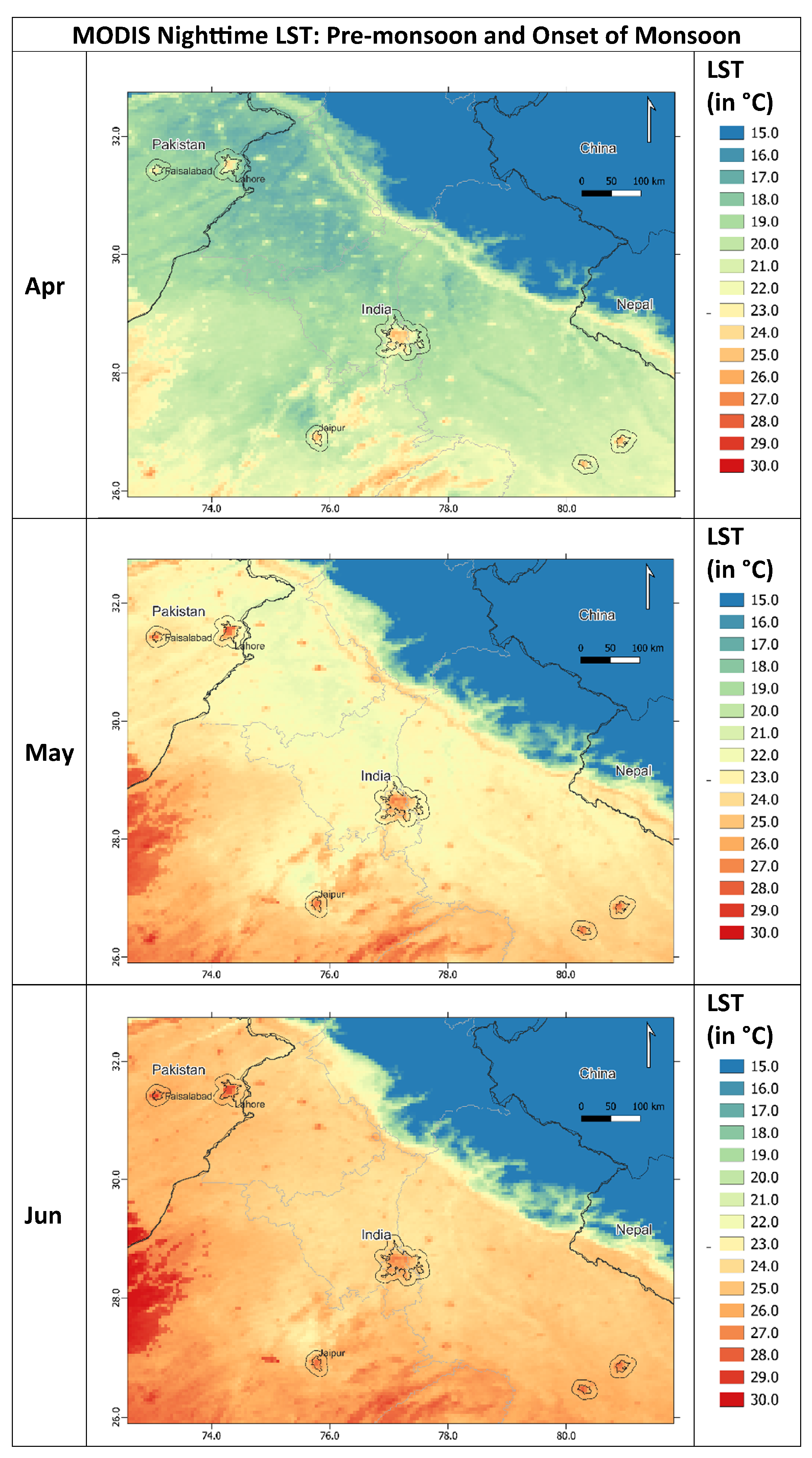
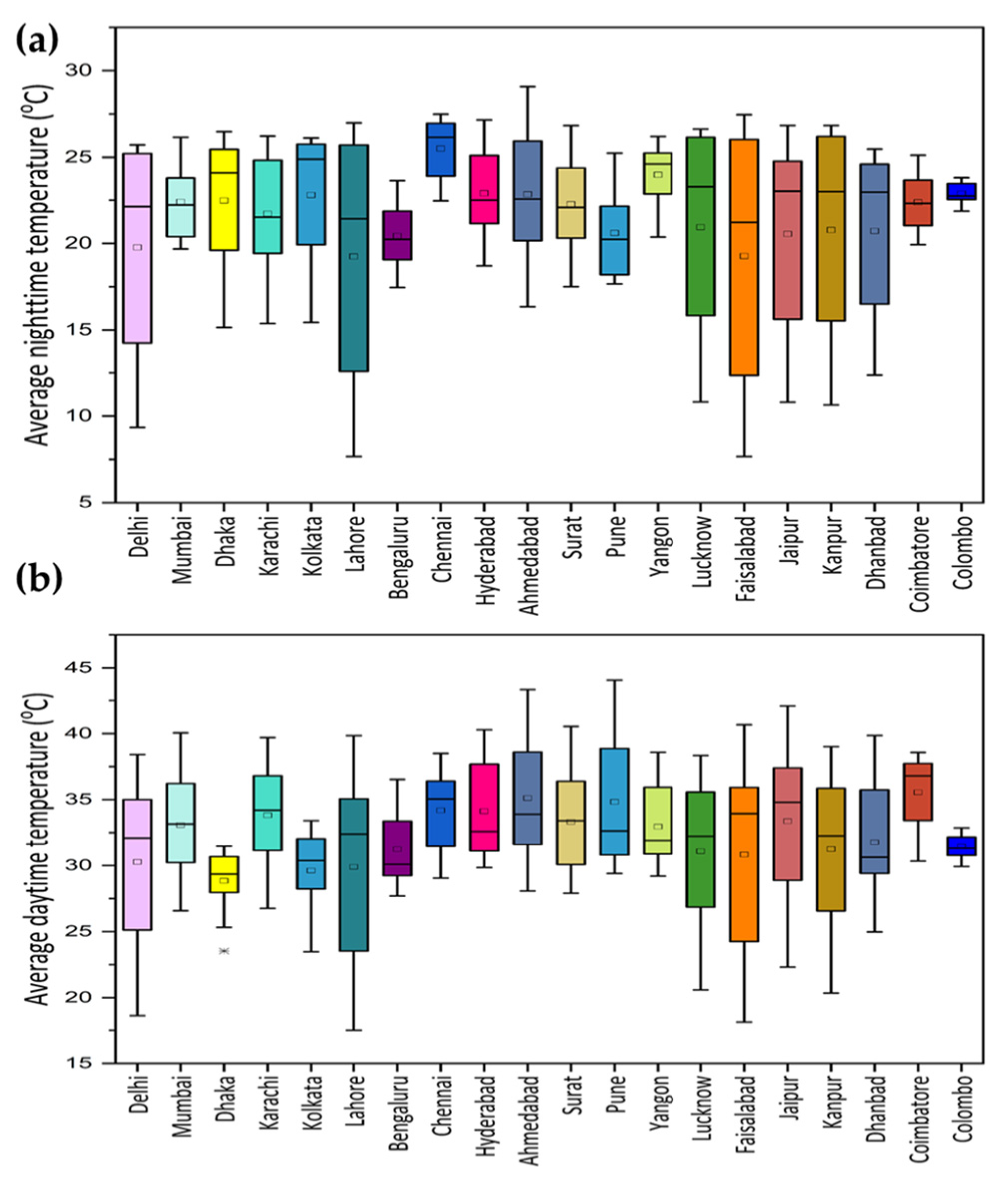
3.1. Spatial Variability of Annual and Seasonal Mean LST

3.1.1. Nighttime LST

The average nighttime LST showed contrasting variability across months and seasons. The climatological annual mean of nighttime LST over the studied major cities in India and surrounding countries ranged from 19.25 °C in Lahore to 25.48 °C in Chennai. As depicted in Figure 1a, the Thar desert and Kutch region showed the highest nighttime warming over the Indian subcontinent (>30 °C) for AMJ (April–May–June) which represents the pre-monsoon to onset of monsoon months. Except for the high-altitude Himalayan region (1–8 km amsl), the AMJ nighttime temperature over the Indian subcontinent ranged from 15 to 30 °C.

The Western Ghats, also known as the Sahyadri mountain range, covers an area of 160,000 km² in a stretch of 1600 km parallel to the western coast of the Indian Peninsula. A narrow band, 0 to 100 km from the Arabian Sea coast running from Gujarat to Kerala usually shows a warmer temperature compared with the eastern side of the Western Ghats which shows a contrastingly cooler temperature (<20 °C). The northwest–southeast trending LST anomalies are due to the barren land in Rajasthan and Bundelkhand. The foothills of the Himalayas are visibly demarcated by the transition from barren to vegetated land. The valley region is demarcated with a lower LST value. The seasonal progression of warmer LST to north during pre-monsoon and onset of monsoon months (AMJ) is depicted in Figure 2 and Figure 3.

Figure 2 clearly portrays that the highest nighttime warming over India occurred during the month of May specifically in central India and spreading out to northern and northeastern India during June. This gradual warming of nighttime LST from April to June in the northern Indo-Gangetic plains is clearly visible in Figure 2, which indicates the formation of the low-pressure zone leading to the onset of monsoon. July and August showed a substantial drop in nighttime LST due to the monsoons. The monthly average nighttime LST for DJF (December–January–February) representing winter months in the Indian subcontinent is illustrated in Figure 4. January showed relatively lower warming along the northern India and IG plains, while February showed higher warming in these areas during the winter months. Some of the largest agglomerations of northern India and its surrounds such as New Delhi, Jaipur, Kanpur, Faisalabad, and Lahore, showed much higher nighttime (24.47, 25.71, 25.46, 24.80, and 24.69 °C) LST within the city limits compared with their surroundings during AMJ and DJF months, as illustrated in Figure 3 and Figure 4.

The monthly breakdown of the average nighttime temperature as given in

Table 2. Average nighttime temperature (LST, °C) showing the variability of surface temperature across months and seasons.

SI.	City	Ann.	AMJ	DJF	Jan	Feb	Mar	Apr	May	Jun	July	Aug	Sep	Oct	Nov	Dec
1.	Delhi	19.77	24.47	10.95	9.35	12.81	17.71	22.64	25.06	25.71	25.61	25.37	25.01	21.61	15.64	10.69
2.	Mumbai	22.49	25.13	20.62	19.82	21.16	23.54	25.86	26.15	23.38	19.68	19.93	21.55	24.01	22.90	20.86
3.	Dhaka	22.11	24.38	16.71	15.15	18.04	21.58	24.09	24.06	24.99	25.93	26.30	26.47	24.96	21.17	16.95
4.	Karachi	21.72	25.29	16.77	15.38	18.22	21.70	24.92	26.22	24.73	20.63	20.96	24.50	25.25	21.33	16.73
5.	Kolkata	22.57	25.37	17.04	15.44	19.11	23.13	25.27	25.16	25.69	26.11	25.81	25.94	24.62	20.75	16.58
6.	Lahore	19.25	24.69	9.27	7.66	10.84	15.98	21.47	25.62	26.98	26.32	25.79	25.27	21.37	14.33	9.30
7.	Bengaluru	20.44	22.56	18.71	18.34	20.34	22.54	23.62	22.88	21.19	20.14	20.08	20.56	19.78	18.27	17.46
8.	Chennai	25.48	27.37	23.17	22.82	24.24	26.01	27.23	27.37	27.49	26.68	26.34	26.29	25.60	23.53	22.46
9.	Hyderabad	22.89	26.47	20.01	19.39	21.95	24.71	26.76	27.16	25.51	23.27	22.19	22.81	22.02	20.34	18.70
10.	Ahmedabad	22.85	27.82	17.72	16.34	19.22	23.41	27.50	29.08	26.89	21.43	21.71	24.97	24.76	21.10	17.61
11.	Surat	22.29	25.81	18.56	17.51	19.68	22.85	25.91	26.83	24.68	21.25	20.93	23.72	24.07	21.31	18.50
12.	Pune	20.61	23.89	18.52	17.77	20.15	22.81	25.24	24.95	21.49	18.12	18.26	20.33	20.97	19.48	17.66
13.	Yangon	23.59	25.41	21.18	20.37	22.13	24.76	26.20	25.48	24.56	25.02	25.47	24.31	24.67	23.59	21.04
14.	Lucknow	20.90	25.56	12.62	10.82	14.73	19.40	23.93	26.14	26.63	26.22	26.16	25.33	22.61	16.94	12.30
15.	Faisalabad	19.27	24.80	9.13	7.66	10.57	15.73	21.19	25.75	27.46	26.68	26.30	25.40	21.24	14.13	9.16
16.	Jaipur	20.55	25.71	12.49	10.80	14.37	19.38	23.85	26.45	26.84	24.83	23.99	24.72	22.18	16.86	12.28
17.	Kanpur	20.77	25.46	12.31	10.65	14.36	18.72	23.45	26.09	26.83	26.31	26.31	25.40	22.53	16.70	11.93
18.	Dhanbad	20.47	24.88	13.79	12.37	15.83	20.33	24.36	24.80	25.47	24.64	24.57	24.19	21.72	17.17	13.16
19.	Coimbatore	22.39	24.14	21.03	20.41	22.74	24.50	25.12	24.10	23.20	22.18	21.64	22.46	22.02	20.24	19.93
20.	Colombo	22.88	23.26	22.97	22.61	23.53	23.66	23.79	23.37	22.61	21.86	22.03	22.70	22.47	23.11	22.77

(Ann.: Annual; AMJ: April–May–June; DJF: December–January–February).

shows that that the highest nighttime temperatures for most of the cities (Karachi, Bengaluru, Chennai, Hyderabad, Ahmedabad, Surat, and Pune) were recorded during April, May, and June.

Delhi, Dhaka, Kolkata, Lahore, Lucknow, Kanpur, and Dhanbad showed variations with the highest nighttime temperature recorded during the May–September months (Table 2). The highest and lowest average nighttime temperature of major cities during AMJ months was 27.82 °C recorded in Ahmedabad and 22.56 °C recorded in Bengaluru, respectively. Similarly, the lowest nighttime temperatures were recorded during DJF/winter months with the highest temperature recorded in Chennai at 23.17 °C and the lowest in Faisalabad at 9.13 °C. In general, the southern Indian cities such as Bengaluru, Chennai, Pune, Hyderabad, and Coimbatore showed the lowest temperature in the month of December, while the other northern Indian cities of the plains showed the lowest nighttime temperatures during January.

3.1.2. Daytime LST

The annual mean of daytime LST over the studied major cities in India and surrounding countries during 2000–2023 ranged from 28.82 °C in Dhaka to 35.55 °C in Coimbatore. Similar to nighttime temperatures, the average daytime LST showed the variability of surface temperature across months and seasons, with the highest daytime temperature in all cities recorded during March, April, May, and June.

Table 3. Average daytime temperature (LST, °C) showing the variability of surface temperature across months and seasons.

SI.	City	Ann.	AMJ	DJF	Jan	Feb	Mar	Apr	May	Jun	July	Aug	Sep	Oct	Nov	Dec
1.	Delhi	30.26	37.39	21.11	18.61	23.14	29.96	37.34	38.41	36.41	33.60	31.83	32.89	32.35	27.09	21.58
2.	Mumbai	33.29	37.43	32.41	31.15	34.46	38.37	40.05	37.97	34.26	26.58	26.89	29.28	32.92	33.38	31.63
3.	Dhaka	28.82	30.51	25.32	23.53	27.10	30.97	31.47	30.86	29.22	28.81	29.48	29.99	30.48	28.88	25.32
4.	Karachi	33.83	37.86	28.60	26.75	30.48	35.95	39.69	38.43	35.46	32.67	31.80	34.47	37.65	33.93	28.59
5.	Kolkata	29.61	32.73	25.29	23.48	27.71	31.99	33.41	32.69	32.08	29.00	30.05	30.70	30.78	28.73	24.70
6.	Lahore	29.89	37.94	19.64	17.50	21.47	28.27	36.00	39.84	37.97	34.11	32.84	33.31	31.94	25.59	19.96
7.	Bengaluru	31.26	33.82	29.90	29.03	32.98	36.29	36.53	33.76	31.18	29.57	29.42	30.46	29.72	28.16	27.69
8.	Chennai	34.19	37.76	30.65	29.95	32.96	35.78	36.84	37.96	38.50	35.96	34.86	35.24	33.52	29.68	29.05
9.	Hyderabad	34.14	39.22	31.41	30.35	34.05	38.15	40.16	40.28	37.21	32.91	31.40	32.12	32.26	30.80	29.84
10.	Ahmedabad	35.21	41.49	30.02	28.07	32.37	38.75	43.31	42.71	38.45	33.10	30.82	33.90	36.47	33.90	29.64
11.	Surat	33.44	37.75	31.10	29.68	33.16	37.98	40.53	38.59	34.12	28.16	27.90	30.96	34.81	33.64	30.47
12.	Pune	34.88	41.27	32.40	31.07	35.59	40.44	44.03	42.50	37.29	30.28	29.39	31.72	33.00	32.26	30.53
13.	Yangon	33.29	35.89	32.63	31.78	34.82	37.44	38.58	37.05	32.05	31.02	29.55	29.19	30.73	32.07	31.29
14.	Lucknow	31.03	37.53	22.94	20.59	25.41	32.48	38.34	37.60	36.64	34.50	31.77	32.24	32.21	28.30	22.82
15.	Faisalabad	30.82	38.48	20.30	18.12	21.95	28.41	36.31	40.67	38.45	35.52	34.85	35.18	33.04	26.55	20.84
16.	Jaipur	33.37	40.94	24.88	22.31	27.46	34.87	41.35	42.08	39.38	35.20	32.49	34.73	35.43	30.28	24.86
17.	Kanpur	31.22	38.58	22.76	20.36	25.08	32.14	39.01	38.90	37.81	33.91	31.76	32.37	32.64	28.05	22.85
18.	Dhanbad	31.77	37.72	26.80	24.96	29.89	35.82	39.85	37.66	35.65	31.52	30.10	30.58	30.67	28.91	25.55
19.	Coimbatore	35.55	37.69	32.39	31.49	35.34	38.57	38.42	37.57	37.07	36.53	37.22	37.89	35.54	30.66	30.33
20.	Colombo	31.44	31.10	31.47	31.22	32.57	32.86	32.45	30.93	29.93	30.56	31.22	31.69	31.87	31.39	30.63

(Ann.: Annual; AMJ: April–May–June; DJF: December–January–February).

provides the seasonal and monthly breakdown of the average daytime LST. The average daytime LST over India and surrounding countries for AMJ months (Figure 1b) indicated that the Thar desert and Kutch region showed the highest warming (>50 °C) similar to the nighttime temperature pattern, and except for the Himalayan region, the average daytime LST over India ranged from 30 to 50 °C during AMJ. It is also noted that central India showed much higher warming during pre-monsoon to onset of monsoon, compared with other parts of the country. The highest and lowest average daytime temperature of major cities during pre-monsoon months was 41.49 °C recorded in Ahmedabad and 30.51 °C recorded in Dhaka, respectively. The lowest daytime temperatures were recorded during DJF/winter months, with the highest temperature recorded in Coimbatore at 32.39 °C and the lowest in Lahore at 19.64 °C. Similar to nighttime temperature, southern Indian cities such as Bengaluru, Chennai, Pune, Hyderabad, and Coimbatore showed the lowest daytime temperature in the month of December, while the other northern Indian cities showed the lowest daytime temperature during January. It is noted that there were conspicuous seasonal variations in the peaks of the daytime and nighttime temperatures over the cities, with daytime temperature peaking in the pre-monsoon summer months while the nighttime temperature of certain cities (Delhi, Dhaka, Kolkata, Lahore, Lucknow, Kanpur, and Dhanbad) peaked around the pre-monsoon months. A bar chart showing the seasonal average (a) nighttime and (b) daytime temperature is provided in Figure 5.

It is noted from Figure 6 that cities such as Delhi, Lahore, Faisalabad, Lucknow, Kanpur, and Jaipur (northern plains) exhibited high variability and range in average nighttime and average daytime temperature compared with Mumbai, Dhaka, Karachi, Kolkata, Bengaluru, Chennai, Hyderabad, Ahmedabad, Surat, Pune, Yangon, Coimbatore, and Colombo. Cities such as Delhi, Lahore, and Faisalabad showed the highest variability in nighttime average temperatures, ranging from 8.22 °C in January to 26.71 °C in June. Lucknow, Jaipur, Kanpur, Dhanbad, and Ahmedabad showed relatively less variability, and cities such as Hyderabad, Karachi, Kolkata, Mumbai, Dhaka, Chennai, Surat, Pune, Yangon, Coimbatore and Colombo showed the least variability in nighttime temperature.

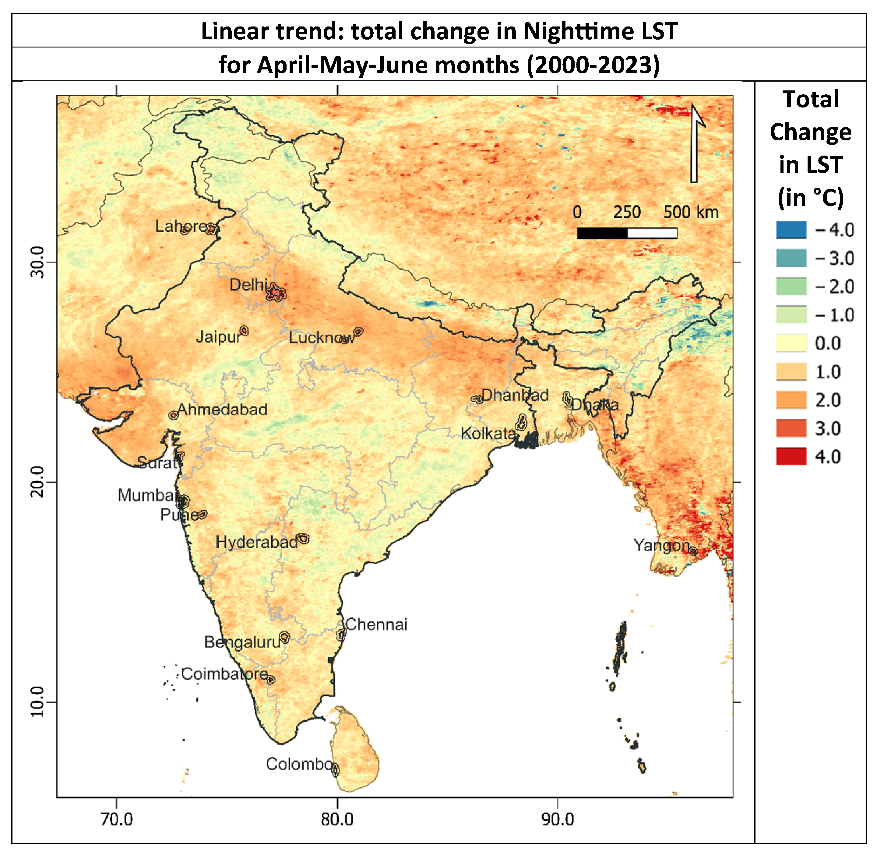
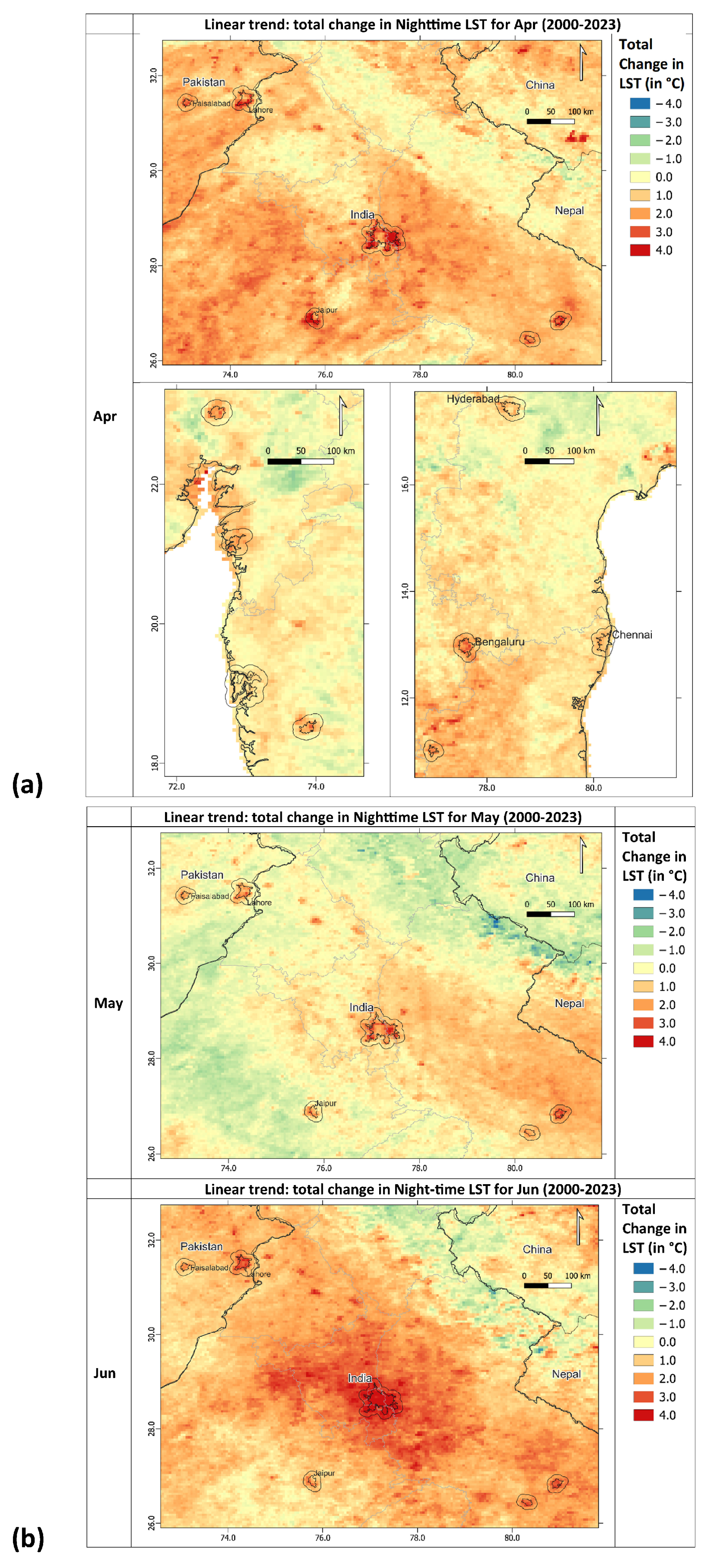
3.2. Spatial and Seasonal Variability of LST Trend

The spatial and seasonal variations in the nighttime and daytime LST trends were computed for the study area. The total change in nighttime MODIS-derived LST over major Indian and other cities for April–May–June months showed conspicuous contrast between major urban city extent, marked as polygons, for the period 2000–2023 (Figure 7).

3.2.1. Nighttime Trend

All urban extents studied showed positive annual trends in nighttime LST (

Table 4. Total change in nighttime temperature (LST, °C) based on the linear trend from 2000–2023.

SI.	City	Ann.	Jan	Feb	Mar	Apr	May	Jun	Jul	Aug	Sep	Oct	Nov	Dec
1.	Delhi	2.02	1.93	2.06	3.53	3.29	2.40	4.58	2.04	1.69	2.56	2.11	1.94	1.20
2.	Mumbai	1.24	0.99	1.28	1.62	0.73	1.23	0.87	4.02	1.41	−0.50	0.94	1.59	1.42
3.	Dhaka	0.09	1.18	−0.16	1.27	1.02	0.39	−0.72	−0.12	−0.81	0.40	−0.07	0.06	0.05
4.	Karachi	1.60	1.16	1.99	2.20	1.62	2.49	2.35	0.65	2.93	2.73	1.31	1.61	1.04
5.	Kolkata	0.91	1.52	0.20	1.99	1.09	1.08	1.14	0.57	0.59	0.94	1.24	1.04	1.00
6.	Lahore	1.68	1.97	2.42	2.57	2.61	1.93	3.01	1.98	1.25	3.24	2.47	1.19	1.18
7.	Bengaluru	1.18	1.40	1.08	2.48	2.37	0.59	1.72	0.90	0.73	0.97	1.18	0.64	2.14
8.	Chennai	1.10	1.57	0.62	1.56	1.30	0.74	1.39	1.48	0.89	1.52	1.11	0.84	1.64
9.	Hyderabad	1.48	1.85	0.56	1.95	1.18	0.94	3.23	1.28	1.55	0.59	1.51	2.62	3.33
10.	Ahmedabad	1.90	1.25	2.39	2.65	2.02	2.18	1.65	7.25	2.21	1.17	1.86	1.82	1.17
11.	Surat	1.94	1.87	2.34	2.74	1.81	1.77	1.39	5.18	0.92	1.69	2.06	2.78	2.39
12.	Pune	1.59	2.12	1.32	2.08	1.79	2.10	1.66	3.63	−0.02	0.76	1.20	2.20	2.67
13.	Yangon	1.56	1.66	0.81	1.80	1.23	2.42	3.83	2.05	10.49	0.34	0.58	2.82	2.41
14.	Lucknow	1.72	1.88	1.51	3.44	3.35	2.89	2.97	1.14	1.72	2.20	2.25	2.01	1.29
15.	Faisalabad	1.43	1.71	1.95	2.65	2.69	1.71	2.06	1.47	1.53	3.23	2.04	1.25	0.72
16.	Jaipur	1.35	1.42	2.21	3.01	2.93	1.71	1.86	3.15	0.67	1.00	1.70	1.43	0.27
17.	Kanpur	1.32	1.32	1.25	2.57	2.46	1.76	2.73	1.75	1.26	1.44	1.51	1.60	0.71
18.	Dhanbad	0.53	1.51	−0.05	2.18	1.43	0.57	2.33	0.79	0.97	0.77	0.67	0.95	0.86
19.	Coimbatore	1.17	1.45	0.74	1.90	2.15	1.00	1.07	2.29	−0.41	0.70	1.06	1.10	2.15
20.	Colombo	0.83	0.99	0.67	0.07	1.58	0.43	0.87	1.00	1.25	1.29	0.51	0.53	1.05

(Ann.: Annual).

), with Delhi witnessing the highest change rate in 23 years (2.02 °C), followed by Surat (1.94 °C), Ahmedabad (1.90 °C), Lucknow (1.72 °C), Lahore (1.68 °C), and Karachi (1.60 °C). A bar chart showing the (a) annual and (b) seasonal (May–June–July, MJJ) total change in nighttime and daytime MODIS-derived LST over major cities for the period 2000–2023 is provided in Figure 8.

Nighttime LST showed an increasing trend in most parts of the country and surroundings with a total change of >3 °C in densely populated urban agglomerates during MJJ months (Figure 7 and Figure 8). Based on the linear fit, it can be clearly observed from Figure 7 that the northern Indo-Gangetic flat plains (Delhi, Haryana, Uttar Pradesh, Jaipur) and western Kutch region (Gujarat) have undergone much higher warming (1–4 °C) in the past 23 years for the AMJ months than the rest of the study.

Significant seasonal variations in the total change of nighttime LST over these cities were observed with the pre-monsoon (March–April–May) and monsoon (June–July) seasons (Figure 8b) showcasing an average higher sporadic pocket of warming except for Dhaka (−0.15 C°), while the winter season showed a relatively lesser warming trend.

The total change in nighttime LST for April, May, and June are individually represented in Figure 9, which clearly depicts the effect of SUHI over urban cities. The linear trend of nighttime LST inside all the city limits was visibly much higher than the surrounding 10 km buffer zone for all months, while rural areas showed a negative or nil trend. There were spatial and seasonal variations in the linear trend of nighttime LST over Indian cities and surrounding cities. Apart from the cities marked in Figure 9, adjacent two and three-tier cities such as Amritsar, Jalandhar, Aligarh, Agra, Ludhiana, Meerut, and Bareilly in the northwestern plains of India could be identified as showing the SUHI effect visible in temporal trend analysis. Along the northwestern plains of India, June showed one of the highest total changes in warming nighttime LST, with Delhi exhibiting >4 °C change.

3.2.2. Daytime Trend

The annual and monthly breakdown of daytime LST over the studied cities are given in

Table 5. Total change in daytime temperature (LST, °C) based on the linear trend from 2000–2023.

SI.	City	Ann.	Jan	Feb	Mar	Apr	May	Jun	Jul	Aug	Sep	Oct	Nov	Dec
1.	Delhi	−0.81	−0.67	−0.12	0.66	0.15	0.93	2.42	0.90	−0.17	0.13	−0.82	−2.12	−2.08
2.	Mumbai	−1.38	−1.71	−1.54	−1.39	−1.44	−0.51	−1.47	0.72	−1.51	−0.17	−0.89	−1.75	−2.16
3.	Dhaka	1.50	0.80	0.42	2.16	3.18	2.66	3.66	3.69	1.14	2.30	1.44	1.49	−0.30
4.	Karachi	−1.28	−2.28	−0.36	−0.98	−0.73	1.21	0.01	−1.17	0.85	−1.15	−2.18	−1.97	−1.42
5.	Kolkata	0.61	0.36	−0.53	0.93	1.75	1.47	2.20	1.67	0.46	1.70	1.53	0.94	−0.37
6.	Lahore	−0.23	−0.60	−0.03	0.37	0.16	0.41	3.05	2.83	1.12	0.92	0.08	−1.01	0.22
7.	Bengaluru	−1.37	−1.71	−3.37	−1.92	−0.92	−2.21	−1.67	−0.39	1.37	−0.40	0.13	−0.53	−1.09
8.	Chennai	−0.37	0.25	−0.27	0.65	0.25	−0.83	−0.66	−0.66	−0.36	−0.25	0.71	0.65	0.60
9.	Hyderabad	−1.90	−1.93	−2.97	−1.19	−2.34	−3.47	−0.99	0.23	0.62	−0.29	−1.13	−1.85	−2.33
10.	Ahmedabad	−1.60	−2.07	−1.08	−1.40	−1.11	0.49	−0.34	−0.83	2.13	−1.67	−2.55	−1.94	−2.58
11.	Surat	−0.62	−1.36	−1.13	−0.73	−0.61	1.61	−1.50	2.53	1.02	−0.09	−1.24	−0.97	−1.99
12.	Pune	−3.25	−3.43	−4.88	−4.60	−4.38	−2.86	−2.87	3.05	−1.61	−1.49	−2.72	−3.50	−3.82
13.	Yangon	0.32	−0.11	−0.89	−0.54	−1.36	2.50	4.65	3.41	−0.35	1.50	0.22	1.21	0.59
14.	Lucknow	−0.59	−1.30	−0.73	−0.12	−0.41	1.26	2.33	4.16	−0.37	2.44	−0.28	−1.48	−2.27
15.	Faisalabad	−0.29	−0.43	0.22	0.43	−0.75	−0.20	2.47	2.25	1.06	0.76	0.40	−0.73	0.66
16.	Jaipur	−2.37	−2.48	−1.27	−1.92	−1.42	0.27	0.63	0.65	−1.12	−2.67	−3.33	−3.31	−3.51
17.	Kanpur	−0.89	−1.39	−1.40	−0.18	−0.88	1.62	2.34	3.89	−1.28	1.08	−0.81	−1.94	−2.06
18.	Dhanbad	−1.21	−1.13	−2.51	−1.09	−1.29	−1.06	1.66	−0.35	−0.39	0.48	0.67	−0.55	−2.21
19.	Coimbatore	−1.75	−1.47	−2.95	−0.46	−0.41	−1.51	−0.97	−3.42	−1.86	−3.24	−0.53	0.56	−1.09
20.	Colombo	1.57	1.28	1.40	1.80	1.93	1.97	1.27	1.80	2.22	0.65	1.83	1.18	1.59

(Ann.: Annual).

. The monthly breakdown of the daytime LST shows that pre-monsoon and monsoon (May–June–July) months showed a positive daytime LST trend for most cities except for Ahmedabad, Mumbai, Pune, Hyderabad, Chennai, Bengaluru, and Coimbatore (Table 1).

Although the annual total change in daytime LST for 23 years was negative except for Dhaka (1.50 °C), Kolkata (0.61 °C), Yangon (0.32 °C), and Colombo (1.57 °C), the total change in daytime LST for May–June–July was relatively highly positive in Yangon (3.52 °C), followed by Dhaka (3.34 °C), Kanpur (2.62 °C), Lucknow (2.58 °C), Lahore (2.10 °C), Kolkata (1.78 °C), and other cities (Table 1).

3.3. Spatial Variability of Annual and Seasonal SUHI

A higher LST in urban extent can be demarcated from Figure 9, which reports the LST trend in the study area. The LST anomaly, calculated as the difference in LST between the urban extent and the surrounding buffer of 10 km, also clearly indicated the effect of surface urban heat island occurring in all cities studied. The diurnal and seasonal variation in SUHI characteristics were also noted in the present study.

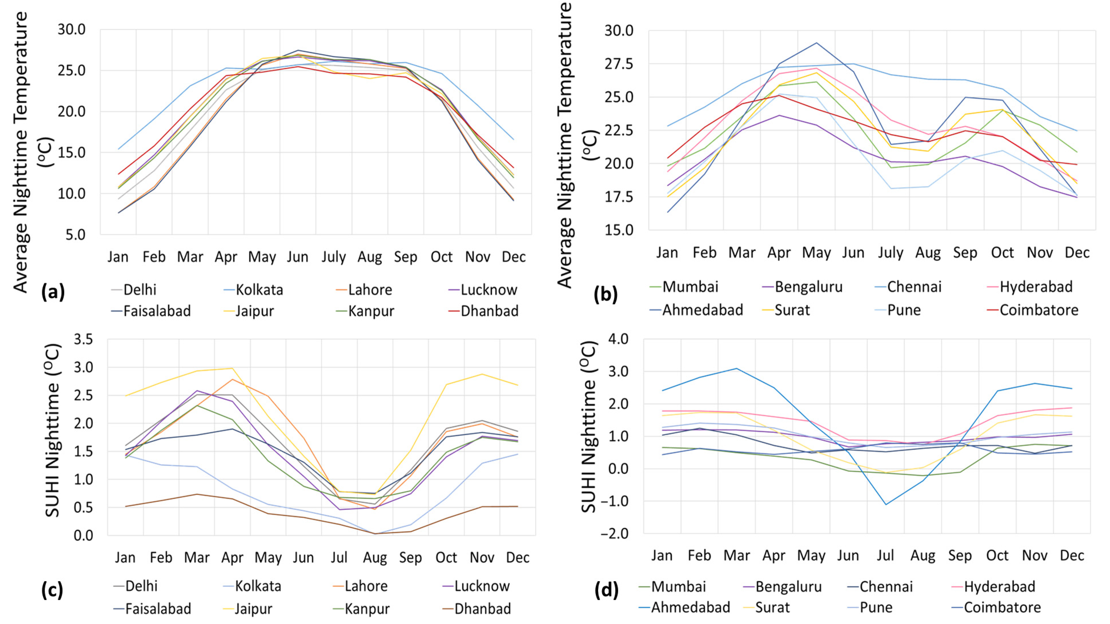
3.3.1. Nighttime SUHI

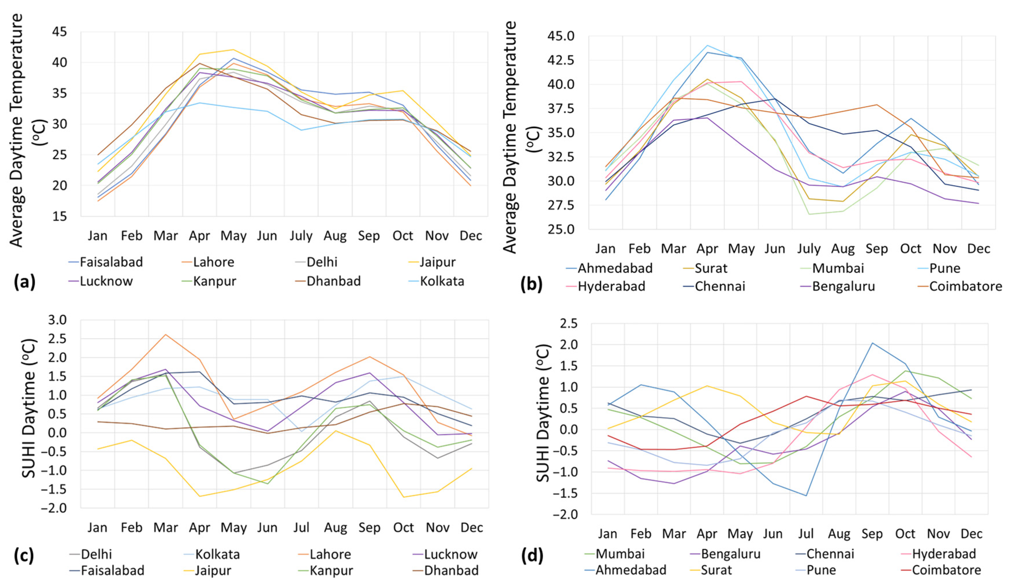
The SUHI, calculated by comparing the average nighttime LST of the urban core with the minimum nighttime LST of surrounding non-urban areas, exhibits the effects of rapid urbanization. The annual nighttime SUHI effect was positive for all the cities, with the highest intensity observed in Jaipur (2.17 °C), followed by Lahore (1.70 °C), Ahmedabad (1.69 °C), Delhi (1.67 °C), Lucknow (1.50 °C), Faisalabad (1.49 °C), Hyderabad (1.47 °C), and Kanpur (1.43 °C) (

Table 6. Nighttime surface thermal anomaly showing urban heat island (SUHI_Mean) effect (average LST_urban − average LST_rural).

SI.	City	Ann.	AMJ	DJF	Jan	Feb	Mar	Apr	May	Jun	Jul	Aug	Sep	Oct	Nov	Dec
1.	Delhi	1.67	1.87	1.84	1.60	2.06	2.51	2.51	1.88	1.24	0.66	0.56	1.17	1.91	2.05	1.86
2.	Mumbai	0.34	0.20	0.66	0.65	0.62	0.50	0.39	0.27	−0.07	−0.13	−0.22	−0.11	0.64	0.75	0.71
3.	Dhaka	0.53	0.32	0.94	0.98	0.98	0.91	0.55	0.28	0.12	−0.32	0.03	0.10	0.37	0.78	0.85
4.	Karachi	0.60	0.30	1.29	1.31	1.32	1.03	0.74	0.24	−0.08	−0.45	−0.50	0.14	0.95	1.25	1.24
5.	Kolkata	0.85	0.61	1.38	1.43	1.26	1.23	0.83	0.55	0.44	0.31	0.02	0.19	0.67	1.29	1.45
6.	Lahore	1.70	2.33	1.68	1.45	1.84	2.31	2.79	2.48	1.74	0.66	0.47	1.07	1.85	1.99	1.76
7.	Bengaluru	0.99	0.92	1.15	1.19	1.21	1.20	1.12	0.97	0.67	0.77	0.82	0.87	0.98	0.97	1.07
8.	Chennai	0.75	0.60	1.00	1.04	1.24	1.05	0.72	0.49	0.58	0.52	0.63	0.71	0.72	0.48	0.72
9.	Hyderabad	1.47	1.32	1.81	1.78	1.78	1.75	1.60	1.46	0.89	0.87	0.74	1.07	1.64	1.81	1.88
10.	Ahmedabad	1.69	1.47	2.56	2.41	2.81	3.09	2.50	1.42	0.49	−1.10	−0.38	0.84	2.40	2.63	2.47
11.	Surat	1.05	0.65	1.67	1.64	1.73	1.72	1.18	0.58	0.19	−0.11	0.04	0.60	1.41	1.66	1.62
12.	Pune	1.03	1.01	1.27	1.28	1.41	1.37	1.26	0.99	0.80	0.66	0.71	0.78	0.96	1.06	1.14
13.	Yangon	0.84	0.33	1.36	1.29	1.58	1.35	0.84	0.58	−0.41	−0.49	1.08	−0.37	0.14	0.82	1.22
14.	Lucknow	1.50	1.69	1.72	1.42	2.03	2.58	2.39	1.62	1.05	0.46	0.50	0.75	1.40	1.77	1.69
15.	Faisalabad	1.49	1.61	1.67	1.53	1.73	1.79	1.90	1.63	1.30	0.78	0.75	1.11	1.76	1.84	1.76
16.	Jaipur	2.17	2.17	2.63	2.49	2.73	2.93	2.98	2.13	1.42	0.79	0.73	1.52	2.69	2.88	2.68
17.	Kanpur	1.43	1.42	1.64	1.38	1.88	2.32	2.06	1.33	0.88	0.68	0.66	0.80	1.49	1.75	1.67
18.	Dhanbad	0.39	0.45	0.55	0.52	0.62	0.74	0.65	0.39	0.32	0.20	0.03	0.07	0.31	0.52	0.52
19.	Coimbatore	0.57	0.53	0.53	0.43	0.63	0.52	0.44	0.53	0.61	0.80	0.75	0.80	0.48	0.46	0.52
20.	Colombo	0.21	0.21	0.33	0.31	0.39	0.19	0.21	0.20	0.23	0.10	0.11	0.37	−0.09	0.19	0.30

(Ann.: Annual; AMJ: April-May–June; DJF: December–January–February).

).

A monthly time series plot of nighttime SUHI of the different studied cities is plotted in Figure 10. The spatial variability in the seasonal characteristics of nighttime SUHI is visibly evident from Figure 10, where inland cities such as Delhi, Jaipur, Faisalabad and Lahore observed much higher change in nighttime LST, while coastal cities such as Chennai and Mumbai observed relatively lesser change in nighttime LST. The seasonal characteristics of nighttime SUHI also showed varied behavior for different cities. Colombo, Chennai, Mumbai, Ahmedabad, Yangon, Coimbatore, Pune, and Hyderabad exhibited much higher SUHI effect during winter than during pre-monsoon and onset of monsoon (AMJ) months, while Dhaka, Lahore, Faisalabad, Lucknow, and Delhi showed highest SUHI during February–March months (Table 6). Kolkata, Chennai, Pune, Dhanbad, Hyderabad, Surat, Mumbai, Bengaluru, Karachi, and Ahmedabad were observed to have peak SUHI effect during post-monsoon months (September–October–November).

3.3.2. Daytime SUHI

The daytime observation of the annual SUHI anomaly over Indian cities and surrounding cities was found to be positive in some cities and negative in the rest. Colombo (1.36 °C) showed the highest annual daytime SUHI effect followed by Lahore (1.22 °C), Dhaka (0.95 °C), Kolkata (0.95 °C), Faisalabad (0.92 °C), Yangon (0.83 °C), and Lucknow (0.80 °C). Pune, Hyderabad, Bengaluru, Karachi, and Jaipur were found to have a negative annual daytime SUHI effect of −0.13, −0.26, −0.33, −0.48, −0.92 °C, respectively (

Table 7. Daytime surface thermal anomaly showing urban heat island (SUHI_Mean) effect (average LST_urban − average LST_rural).

SI.	City	Ann.	AMJ	DJF	Jan	Feb	Mar	Apr	May	Jun	Jul	Aug	Sep	Oct	Nov	Dec
1.	Delhi	0.09	−0.77	0.58	0.66	1.36	1.57	−0.38	−1.07	−0.86	−0.47	0.42	0.85	−0.11	−0.67	−0.28
2.	Mumbai	0.16	−0.67	0.49	0.47	0.28	−0.05	−0.42	−0.81	−0.78	−0.40	0.30	0.74	1.38	1.22	0.73
3.	Dhaka	0.95	0.96	0.80	0.70	1.10	1.11	1.21	1.08	0.60	0.90	1.14	1.00	1.00	0.85	0.61
4.	Karachi	−0.48	−0.49	−0.53	−0.53	−0.47	−0.53	−0.37	−0.47	−0.63	−0.83	−0.37	−0.12	−0.38	−0.53	−0.59
5.	Kolkata	0.95	0.99	0.73	0.63	0.94	1.17	1.22	0.88	0.88	0.03	0.73	1.38	1.50	1.05	0.63
6.	Lahore	1.22	1.01	0.84	0.92	1.69	2.61	1.95	0.36	0.72	1.09	1.61	2.02	1.54	0.28	−0.08
7.	Bengaluru	−0.33	−0.65	−0.71	−0.74	−1.15	−1.27	−0.98	−0.39	−0.58	−0.46	−0.08	0.54	0.90	0.49	−0.23
8.	Chennai	0.40	−0.18	0.63	0.62	0.32	0.26	−0.11	−0.32	−0.11	0.25	0.67	0.78	0.69	0.82	0.94
9.	Hyderabad	−0.26	−0.93	−0.84	−0.91	−0.97	−0.99	−0.94	−1.04	−0.80	0.07	0.94	1.29	0.97	−0.04	−0.64
10.	Ahmedabad	0.32	−0.56	0.53	0.58	1.05	0.88	0.18	−0.59	−1.27	−1.56	0.49	2.04	1.55	0.29	−0.03
11.	Surat	0.45	0.66	0.17	0.03	0.31	0.70	1.03	0.79	0.17	−0.07	−0.11	1.03	1.14	0.60	0.18
12.	Pune	−0.13	−0.53	−0.31	−0.31	−0.48	−0.77	−0.84	−0.68	−0.07	0.16	0.69	0.67	0.41	0.11	−0.15
13.	Yangon	0.83	0.34	0.41	0.49	0.11	−0.54	−0.90	−0.12	2.03	1.92	1.92	1.50	2.15	1.64	0.62
14.	Lucknow	0.80	0.36	0.72	0.80	1.39	1.69	0.71	0.33	0.05	0.69	1.33	1.59	0.80	−0.06	−0.02
15.	Faisalabad	0.92	1.07	0.66	0.61	1.17	1.59	1.62	0.77	0.81	0.98	0.81	1.06	0.94	0.51	0.19
16.	Jaipur	−0.92	−1.48	−0.52	−0.43	−0.20	−0.68	−1.69	−1.51	−1.24	−0.75	0.05	−0.33	−1.71	−1.57	−0.95
17.	Kanpur	0.14	−0.91	0.60	0.59	1.41	1.52	−0.32	−1.07	−1.35	−0.35	0.65	0.75	0.06	−0.38	−0.19
18.	Dhanbad	0.32	0.10	0.33	0.30	0.24	0.10	0.15	0.18	−0.02	0.14	0.22	0.55	0.78	0.69	0.44
19.	Coimbatore	0.21	0.06	−0.08	−0.14	−0.46	−0.47	−0.39	0.13	0.43	0.79	0.56	0.59	0.69	0.50	0.36
20.	Colombo	1.36	1.25	1.27	1.33	1.17	1.00	1.16	1.26	1.31	1.62	1.67	1.54	1.64	1.31	1.32

(Ann.: Annual; AMJ: April–May–June; DJF: December–January–February).

).

The monthly time series plot for the daytime SUHI over different cities is plotted in Figure 11, which shows the spatial variability in the seasonal characteristics of daytime SUHI. It can be clearly delineated from Figure 11a,b that the average daytime temperature peaked during pre-monsoon to onset of monsoon months (March–April–May–June) months and post-monsoon, with a prominent dip in temperatures during monsoon months due to heavy rainfall and also during winter months.

4. Discussion

The present study analyzed the annual and seasonal characteristics of the average nighttime and daytime LST, its trend (in terms of total change), and SUHI effects, for over 20 major urban agglomerations in India and surrounding countries for a period of 23 years (2000 to 2023). The study revealed an evident warming trend in all cities during nighttime, while cooling trends were observed in most cities during daytime (except for Dhaka, Kolkata, Yangon, and Colombo, which observed a total change of 1.50, 0.61, 0.32 and 1.57 °C, respectively) over the past two decades (Table 1). This is in agreement with previous LST studies, particularly over Pune, Kolkata, Jaipur, Ahmedabad and Bangalore, which revealed a general nighttime warming trend in all of the above cities, but a daytime warming trend in Kolkata and Ahmedabad and a daytime urban cooling trend in Pune, Jaipur and Bangalore [88,94,95,96]. Daytime urban cooling has also been reported by scientists specifically for the majority of urban regions in central India and the Indo-Gangetic basin [89].

LST is a product of the interplay between various climatic and environmental factors with the land surface, which is seemingly impacted by both atmospheric and land processes. Daytime and nighttime LST values are influenced by different degrees of these interactions. The daytime LST change was found to be affected by factors that exhibit less variability in space but more variability in time, such as solar radiation, while the nighttime LST change was found to be governed by factors that exhibit more variability in space but less variability in time, such as longwave radiation exchange, land cover change, and soil moisture change [97]. An SUHI intensity study across 150 major cities in India, each located in distinct climatic regions, analyzed by employing MODIS data spanning from 2003 to 2018, found that daytime SUHI was tightly linked to vegetation, evapotranspiration, and thermal inertia, while nighttime SUHI was linked with built-up intensity, white sky albedo, and thermal inertia [90]. The nighttime UHI effect and its intensity observed in the present study were more conspicuous, positive, and consistent compared with daytime satellite observations, which agrees with the previous studies and suggests that nighttime LST is more sensitive to changes in urban microclimate and hence a better indicator of SUHI intensity.

Cities located in the Indo-Gangetic plains showed seasonal variation in daytime LST with a rising trend in LST during pre-monsoon to monsoon months and a decreasing trend in post-monsoon to winter months (Table 1 and Table 5). The present study is consistent with the reports of [98], which stated that a decline in daytime LST over the GRB and central India from 2001 to 2019 was partially attributable to rising aerosol trends except for higher sporadic pockets of warming observed in pre-monsoon and monsoon months. The rising trend in AOD over GRB during winter and post-monsoon season and its declining trend in pre-monsoon and monsoon season can be negatively correlated with the daytime LST trend [99]. The decline in daytime LST compared with the significant rise in nighttime LST over the same region suggests that nighttime temperature is more sensitive as a climate change indicator than daytime temperature [100]. The decreased precipitation observed in recent decades, especially during the monsoon months, is speculated to be a possible reason for rising LST in the monsoon. The elevation in net radiation absorption, coupled with increasingly arid climatic conditions, amplifies the warming effect due to reduced cloud cover and diminished moisture availability for evaporative cooling, resulting in higher LST [98]. Previous works of literature have found a decreasing trend in summer rainfall over GRB and central India [101,102].

The present study found that the highest nighttime surface urban island effect was observed in Jaipur, Delhi, Lucknow, Lahore, Faisalabad, Kanpur, and Dhanbad during the pre-monsoon (March–April–May) months (Figure 9 and Figure 10, Table 6), although the highest average nighttime temperatures recorded in these cities were in April–May–June, while Ahmedabad, Hyderabad, Surat, Kolkata, Yangon, Karachi, Pune, Bengaluru, Chennai, Dhaka, Mumbai, Coimbatore, and Colombo exhibited the highest effect of urban heat island during winter. The study points out that all cities uniformly exhibited higher nighttime SUHI during winter months than during AMJ in all cities except Lahore. Delhi exhibited slightly less nighttime SUHI in winters than during AMJ. The nighttime SUHI effect was observed to be lowest in all cities during the peak monsoon (June–July–August) months (Figure 10c).

It can be clearly demarcated from Figure 10a,b that average nighttime temperature patterns varied along different months over different cities. Delhi, Kolkata, Lahore, Lucknow, Faisalabad, Jaipur, Kanpur, and Dhanbad were observed to have peak nighttime temperatures during MJJ months, which were maintained throughout the monsoon season. The nighttime LST of these regions was observed to decrease only during winter months. Contrary to this, the nighttime SUHI effect peaked with a significant dip in SUHI during monsoon season for cities such as Mumbai, Ahmedabad, Surat, Bangalore, Coimbatore, and Hyderabad (Figure 10d). These cities showed relatively higher SUHI during winter months.

The daytime SUHI variability showed strong contrast compared with the nighttime SUHI (Figure 10 and Figure 11). Karachi, Bengaluru, Hyderabad, Pune, and Jaipur exhibited negative daytime SUHI in both pre-monsoon to onset of monsoon months and during winter months. Karachi, Bengaluru, Hyderabad, Pune, and Jaipur showed highly contrasting diurnal behaviors with a negative daytime SUHI effect and a positive nighttime SUHI effect in both seasons. Delhi, Mumbai, Ahmedabad, and Kanpur showed daytime negative SUHI during pre-monsoon to onset of monsoon months, and positive SUHI during winter. Cities such as Colombo, Yangon, Lucknow, Kolkata, Dhaka, Lahore, Faisalabad, Surat, and Dhanbad showed positive SUHI during daytime and nighttime in both seasons.

The daytime SUHI observations for Delhi, Kolkata, Lahore, Lucknow, Faisalabad, Jaipur, and Kanpur showed the highest peak during March, gradually decreasing during April–May–June–July, and peaking again during post-monsoon months. Mumbai, Bengaluru, Chennai, Hyderabad, Ahmedabad, Surat, Pune, and Coimbatore were observed to have the highest daytime SUHI effect during post-monsoon months and a relatively lesser peak during winter months. The daytime SUHI showed a much more complex pattern over the months compared with nighttime SUHI for all cities. Figure 12a,b shows the variability of nighttime and daytime SUHI over the studied cities.

In India, Jaipur exhibited the highest nighttime SUHI during pre-monsoon to onset of monsoon (2.17 °C) months and during winter (2.63 °C). Similarly in Pakistan, Lahore showed higher nighttime SUHI during AMJ months than in Faisalabad and Karachi. It is noted that the nighttime SUHI effect was more pronounced than the daytime SUHI effect for all cities in and surrounding India except Colombo, as depicted in Figure 13. The highest nighttime SUHI exhibited by Delhi was during March and April (2.51 °C), and the lowest nighttime SUHI was during August. Lucknow and Kanpur are two closely located cities which exhibit anomalous seasonal daytime SUHI characteristics. Lucknow behaved as an urban heat island during AMJ months with an intensity of 0.36 °C (Figure 13).

It is interesting to note that Karachi and Jaipur, having similar desert to semi-arid climate classification, show daytime negative SUHI effect in almost all months, which points out that the surrounding non-urban areas of these cities are warmer than the city core for all months. Both cities show a similar daytime urban cool island (UCI) effect in winter months (−0.52 to −0.53 °C), while during pre-monsoon to onset of monsoon, Jaipur shows much higher daytime negative UHI effect (−1.48 °C) compared with Karachi (−0.49 °C). This result agrees with the earlier literature that observed a significant role of thermal admittance of rural areas in creating a heat island effect. As the thermal admittance values of moist soil are similar to those of typical dense urban building materials, the temperature ranges within the urban area are comparable to those outside it, resulting in a low SUHI intensity. Nevertheless, during nighttime, rural areas have slightly lower temperatures compared with urban areas, indicating a positive SUHI [88]. The coastal setting of Karachi compared with inland Jaipur might also influence the more moderate heat island effect in Karachi than Jaipur.

Dhaka, Kolkata, Faisalabad, Lahore, Dhanbad, Lucknow, and Surat showed positive daytime SUHI for almost all months compared with other cities which showed seasonal positive and negative daytime SUHI. Delhi, Kanpur, and Ahmedabad showed similar seasonal variation in daytime UHI with formation of cool islands or negative SUHI during pre-monsoon, monsoon and November–December months.

The average daytime temperature and SUHI intensity patterns across all months of the year of inland cities, and coastal to near coastal cities, are depicted in Figure 11a,b and Figure 11c,d, respectively. The figure clearly displays the influence of geographical location and its related climatic conditions over the seasonal SUHI intensity, though the extent of variability might depend on other factors. Studies on the effect of vegetation cover over India reveal much less pre-monsoon vegetation cover on the IG plains. During the pre-monsoon summer season, barren rural land has lower albedo compared with built-up regions resulting in high LST, while the same is not true for nighttime as albedo is absent during nighttime [89,103].

Jaipur and Lahore are inland cities, whereas Dhaka and Colombo are near-coastal to coastal cities. The influence of their geographical locations is visible in their total change in annual LST over 23 years and the monthly breakdown of nighttime SUHI. The total change in annual LST over the study period for Colombo and Dhaka was 0.83 and 0.09 °C, while for Jaipur and Lahore was 1.35 and 1.68 °C, respectively. Jaipur and Lahore had highly positive nighttime SUHI during the AMJ and DJF months. Jaipur showed a SUHI of 2.17 °C during AMJ and 2.63 during DJF, while Lahore showed a SUHI of 2.33 °C during AMJ and 1.68 during DJF which significantly weakened during monsoon months (June–July–August). A difference of approximately 2 °C in SUHI was observed between April and August in both cities (Figure 10c and Table 6). This can be seen as a general trend in inland cities. Coastal cities, however, do not show much difference in SUHI patterns over months or seasons. The monthly and seasonal breakup of SUHI for Dhaka and Colombo showed relatively no significant highs or lows. Both cities showed a SUHI effect below 1 °C. Colombo, being very close the coast compared with Dhaka, showed a much more uniform SUHI effect (in the range of 0.1 to 0.39 °C) throughout the months (Table 6).

Ahmedabad and Delhi were among the leading five cities exhibiting the most significant annual nighttime SUHI effect. Delhi, being the most populous and extensively urbanized city in India, gauges its level of urbanization through a substantial increase in population, with a decadal urbanization rate of 26.8% from 2001 to 2011. Projections indicate that Delhi is poised to surpass Tokyo as the world’s most populated city [104]. Ahmedabad, characterized as an industrial hub, ranks as the seventh-largest metropolitan city in India, accommodating a population of 7.68 million. The influence of urbanization is evident from the strong positive nighttime SUHI observed in both cities annually and seasonally (AMJ and DJF). The total change in nighttime LST over 23 years based on linear fit (Table 1) showed a strong positive annual change and a total change of 3.70 °C and 3.01 °C for Ahmedabad and Delhi during MJJ months. Notably, June–July marks the monsoon months during which cities in the country receive substantial rainfall, accompanied by monsoon winds and abundant greenery which collectively help alleviate the formation of SUHI. In contrast with this, the monthly nighttime SUHI presented in Table 6 shows strong positive SUHI even in May, June, and July for both Delhi and Ahmedabad, except with Ahmedabad showing an urban cool island effect only in July, supported by earlier studies [105].

The implications of UHI will be stronger in summers with higher summer temperatures increasing air conditioning and energy demand, further increasing atmospheric pollution. The life quality of low-income families in these cities will deteriorate further given the close connection between the indoor thermal environment and outdoor conditions. The increasing SUHI effect in urban areas leads to heightened heat stress and raises significant concerns. Global warming exacerbating the UHI effect will intensify heatwaves, resulting in more extremely hot days during summer and a direct increase in heat-related illness and mortality rates [105]. This ongoing trend of warmer decades and growing SUHIs will place millions of residents in these cities at significant risk of heat-related illnesses and fatalities in the foreseeable future. Hence, design and development of proper mitigation measures can be introduced in city planning such as optimizing urban morphology and geometry, increasing wetlands and water bodies, using highly reflective roofs and pavements, use of permeable and water-retaining materials for pavements, green walls and roofs, and rational planning of blue-green areas. Several studies have concentrated on the effectiveness of each of these mitigation measures and have proven urban blue-green space to be the potential solution because of its inherent environmental, ecological, and social benefits. Urban parks, integral to urban blue-green spaces, offer benefits such as recreation, humidification, and air purification, while also generating park cooling effects [106]. These effects entail urban parks being cooler than the adjacent urbanized areas. Research has investigated the influence of internal park features and the surrounding 2D/3D landscapes on cooling effects [107,108], offering scientific insights to optimize landscape allocation and enhance cooling effects in city parks for effective UHI mitigation. Highly urbanized cities with dense populations, such as Delhi, Mumbai, Kolkata, and Chennai, can implement urban greening solutions such as vertical gardens, rooftop and terrace gardens, urban agriculture, cool roofs, cool pavements, green buildings, and water spray systems [105,109,110] to efficiently diminish UHI intensity. Emerging megacities such as Hyderabad, Ahmedabad, Surat, Pune, Jaipur, Kanpur, and Coimbatore can incorporate urban blue-green spaces such as urban parks into city planning, taking into account both internal and external surroundings, to effectively mitigate UHI effects. In order to support the United Nations Sustainable Development Goals (SDGs), it is critical that future professionals have an understanding of impending environmental issues, such as urban heat islands, and can devise strategies and technologies that promote sustainable development [111].

5. Conclusions

The current investigation examined the spatiotemporal variations in land surface temperature (LST) data obtained from the MODIS sensor aboard Terra satellites, encompassing both daytime and nighttime observations. This study spanned a 23-year duration, commencing in 2000 and extending through 2023, focusing on the 20 largest agglomerations in India and surrounding countries which were selected based on population (>0.5 million). The annual, seasonal, and diurnal variations in the average daytime and nighttime temperatures, their linear trends and total change in 23 years over India and particularly in the selected cities, were analyzed. The main objective of the study was to assess the nighttime and daytime surface urban heat island intensity of the selected cities by computing the difference in LST between urban and non-urban regions. The study highlights the complex diurnal and seasonal characteristics of SUHI in cities. The important findings from the work are listed as follows:

• The Thar desert and Kutch region in India were the warmest regions identified, with an average nighttime temperature greater than 30 °C and daytime temperature greater than 50 °C for the warmest months, April–May–June;
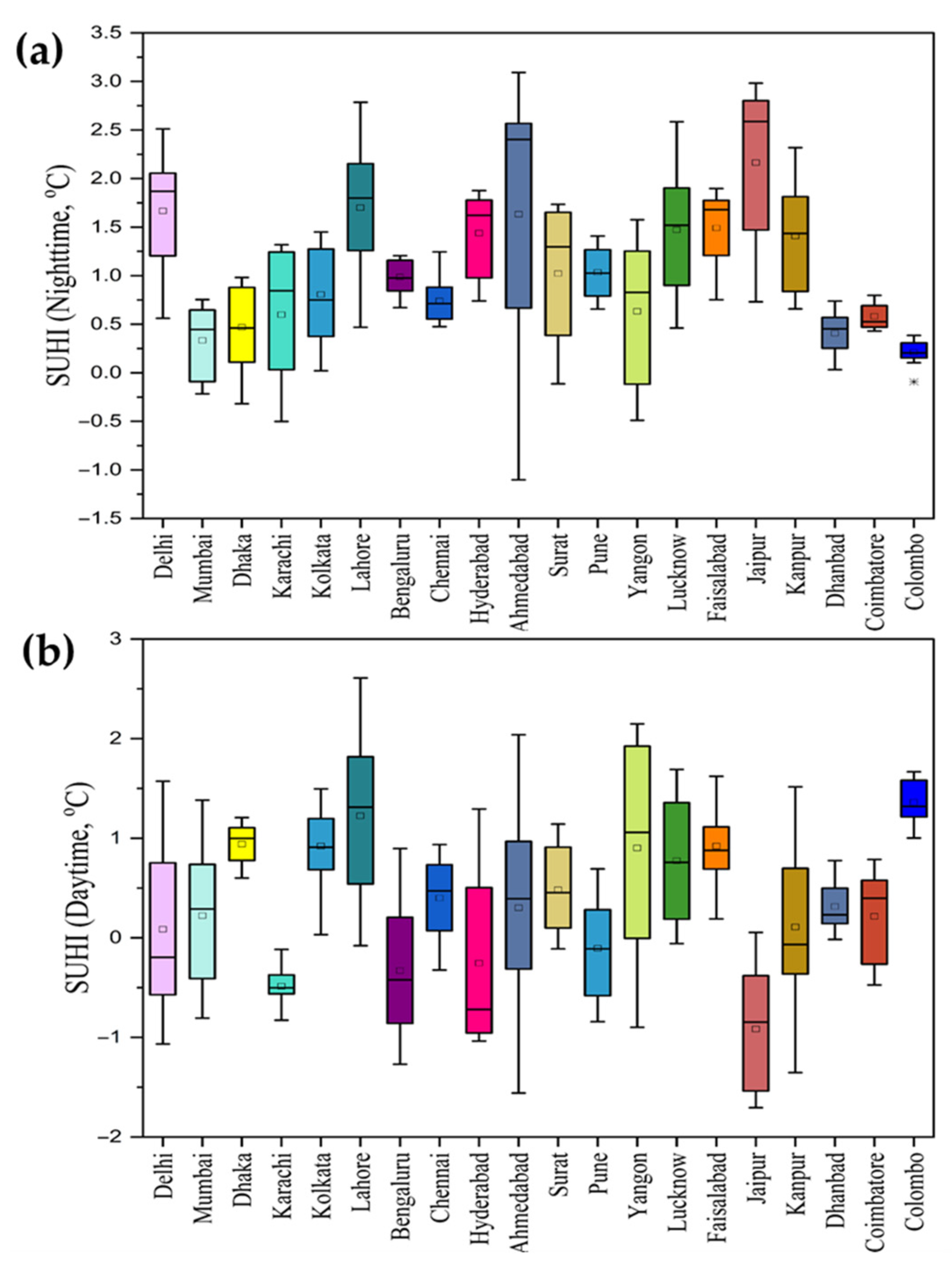
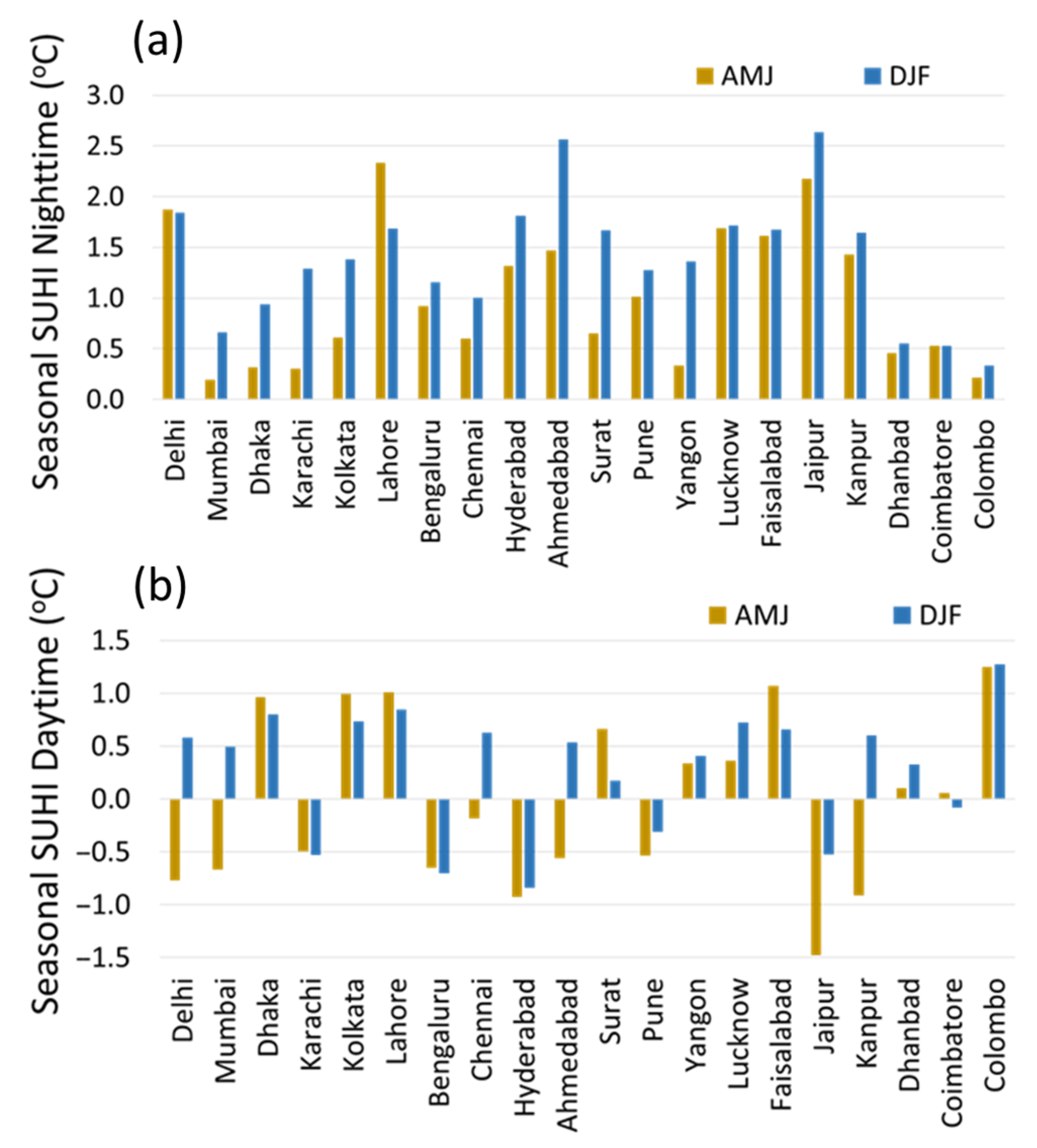
• The nighttime SUHI effect was found to be more conspicuous, positive, and reliable compared with daytime satellite observations, and hence is a more suitable indicator of SUHI effect over cities;
• The annual nighttime temperature trend was observed to be rising in all cities that are expanding, and the highest warming based on trend (statistically significant, 95% CI) was observed in Ahmedabad and Delhi during MJJ (May–June–July) months (3.7 and 3.01 °C, respectively);
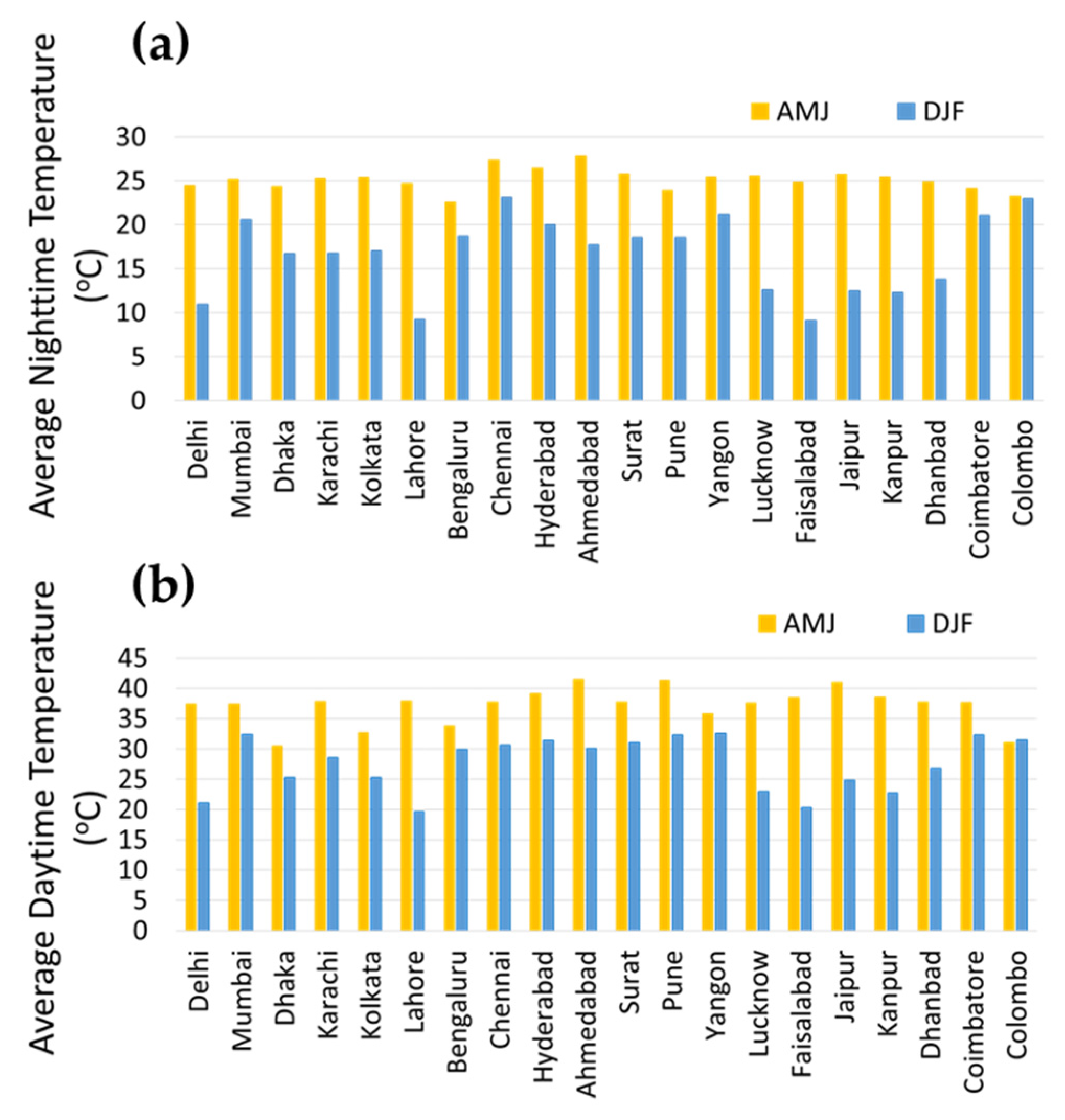
• The nighttime SUHI for AMJ (April–May–June) representing pre-monsoon and onset of monsoon months for the top 10 cities ranged from 0.92 to 2.33 °C, and from 1.38 to 2.63 °C for the winter months (DJF, December–January–February);
• Dhaka, Kolkata, Lahore, Surat, Yangon, Lucknow, Faisalabad, Dhanbad, and Columbo showed positive daytime SUHI, while Mumbai, Karachi, Bengaluru, Chennai, Hyderabad, Ahmedabad, Pune Jaipur, and Kanpur showed negative daytime SUHI during pre-monsoon to onset of monsoon months;
• The seasonal characteristics of daytime SUHI in Delhi, Mumbai, Chennai, Ahmedabad, and Kanpur were negative during pre-monsoon to onset of monsoon, while positive during winter months;
• Inland cities and coastal or near coastal cities showed different patterns of average daytime and nighttime LST pattern by monthly breakdown;
• Monthly daytime SUHI of inland cities such as Delhi, Kanpur, Lahore, Lucknow, Kolkata, Faisalabad, and Jaipur showed two peaks, with a dip during the peak of monsoon and winter season;
• Monthly daytime SUHI of coastal to near coastal cities such as Mumbai, Bengaluru, Chennai, Hyderabad, Pune, and Coimbatore showed the highest peak during post-monsoon;
• In general, all cities uniformly exhibited higher nighttime mean SUHI during DJF (winter months) than that during AMJ months, which otherwise record the highest nighttime LST;
• The monthly or seasonal total change in nighttime LST based on linear trend (2000–2023) exhibited several hotspots not only around the major cities but also around the tier-2 and 3 cities, that can be attributed to rapid urbanization in India.

The complex and different daytime and nighttime SUHI effects across the months in the studied cities are understood to be independent processes with different driving mechanisms. The geographical location of the city seems to have some influence on the daytime and nighttime SUHI patterns as seen from similar patterns of SUHI across months shown by inland and coastal to near coastal cities.

Further scope of work could be the use of higher spatial and temporal resolution satellite datasets from other agencies such as ESA, and JAXA, etc., to decipher the anomalies and trends in SUHI effects. In conjunction with green cover, temporal (diurnal and seasonal) effects can be examined to determine the impact of NDVI on LST and UHI anomalies and trends. These limitations can be overcome through the implementation of multi-sensor investigations that incorporate time series data from both LST and NDVI.

The current research aims to help city planners and policymakers better understand the behaviors of urban heat islands (UHI) during both day and night, on a seasonal basis. This information is crucial for developing strategies to mitigate UHI effects. The processes and mechanisms behind their variations need to be further investigated in detail for urban planning and policy making.

References

1. Helbling, M.; Meierrieks, D. Global Warming and Urbanization. J. Popul. Econ. 2023, 36, 1187–1223. [Google Scholar] [CrossRef]
2. Calvin, K.; Dasgupta, D.; Krinner, G.; Mukherji, A.; Thorne, P.W.; Trisos, C.; Romero, J.; Aldunce, P.; Barrett, K.; Blanco, G.; et al. IPCC, 2023: Climate Change 2023: Synthesis Report. Contribution of Working Groups I, II and III to the Sixth Assessment Report of the Intergovernmental Panel on Climate Change, 1st ed.; Core Writing Team, Lee, H., Romero, J., Eds.; Intergovernmental Panel on Climate Change (IPCC): Geneva, Switzerland, 2023. [Google Scholar]
3. Hopkins, F.M.; Ehleringer, J.R.; Bush, S.E.; Duren, R.M.; Miller, C.E.; Lai, C.-T.; Hsu, Y.-K.; Carranza, V.; Randerson, J.T. Mitigation of Methane Emissions in Cities: How New Measurements and Partnerships Can Contribute to Emissions Reduction Strategies: URBAN METHANE MITIGATION. Earths Future 2016, 4, 408–425. [Google Scholar] [CrossRef]
4. United Nations. World Urbanization Prospects: The 2018 Revision; United Nations: New York, NY, USA, 2019; ISBN 978-92-1-148319-2.
5. Trusilova, K.; Jung, M.; Churkina, G.; Karstens, U.; Heimann, M.; Claussen, M. Urbanization Impacts on the Climate in Europe: Numerical Experiments by the PSU–NCAR Mesoscale Model (MM5). J. Appl. Meteorol. Climatol. 2008, 47, 1442–1455. [Google Scholar] [CrossRef]
6. Wang, H.; Liu, Z.; Wu, K.; Qiu, J.; Zhang, Y.; Ye, B.; He, M. Impact of Urbanization on Meteorology and Air Quality in Chengdu, a Basin City of Southwestern China. Front. Ecol. Evol. 2022, 10, 845801. [Google Scholar] [CrossRef]
7. Tzavali, A.; Paravantis, J.; Mihalakakou, G.; Fotiadi, A.; Stigka, E. Urban Heat Island Intensity: A Literature Review. Fresenius Environ. Bull. 2015, 24, 4537–4554. [Google Scholar]
8. Liao, W.; Li, D.; Malyshev, S.; Shevliakova, E.; Zhang, H.; Liu, X. Amplified Increases of Compound Hot Extremes Over Urban Land in China. Geophys. Res. Lett. 2021, 48, e2020GL091252. [Google Scholar] [CrossRef]
9. Peng, S.; Piao, S.; Ciais, P.; Friedlingstein, P.; Ottle, C.; Bréon, F.-M.; Nan, H.; Zhou, L.; Myneni, R.B. Surface Urban Heat Island Across 419 Global Big Cities. Environ. Sci. Technol. 2012, 46, 696–703. [Google Scholar] [CrossRef]
10. Peng, W.; Wang, R.; Duan, J.; Gao, W.; Fan, Z. Surface and Canopy Urban Heat Islands: Does Urban Morphology Result in the Spatiotemporal Differences? Urban Clim. 2022, 42, 101136. [Google Scholar] [CrossRef]
11. Lee, S.-H.; Baik, J.-J. Statistical and Dynamical Characteristics of the Urban Heat Island Intensity in Seoul. Theor. Appl. Climatol. 2010, 100, 227–237. [Google Scholar] [CrossRef]
12. Oke, T.R. The Energetic Basis of the Urban Heat Island. Q. J. R. Meteorol. Soc. 1982, 108, 1–24. [Google Scholar] [CrossRef]
13. Yang, L.; Qian, F.; Song, D.-X.; Zheng, K.-J. Research on Urban Heat-Island Effect. Procedia Eng. 2016, 169, 11–18. [Google Scholar] [CrossRef]
14. Hassid, S.; Santamouris, M.; Papanikolaou, N.; Linardi, A.; Klitsikas, N.; Georgakis, C.; Assimakopoulos, D.N. The Effect of the Athens Heat Island on Air Conditioning Load. Energy Build. 2000, 32, 131–141. [Google Scholar] [CrossRef]
15. Santamouris, M.; Papanikolaou, N.; Livada, I.; Koronakis, I.; Georgakis, C.; Argiriou, A.; Assimakopoulos, D.N. On the Impact of Urban Climate on the Energy Consumption of Buildings. Sol. Energy 2001, 70, 201–216. [Google Scholar] [CrossRef]
16. Akbari, H. Energy Saving Potentials and Air Quality Benefits of Urban Heat Island Mitigation. In Proceedings of the First International Conference on Passive and LowEnergy Cooling for the Built Environment, Athens, Greece, 17–24 May 2005. [Google Scholar]
17. Santamouris, M. On the Energy Impact of Urban Heat Island and Global Warming on Buildings. Energy Build. 2014, 82, 100–113. [Google Scholar] [CrossRef]
18. Taha, H.; Douglas, S.; Haney, J. The UAM Sensitivity Analysis: The 26–28 August 1987 Oxidant Episode. In Analysis of Energy Efficiency and Air Quality in the South Coast Air Basin–Phase II; Taha, H., Douglas, S., Haney, J., Eds.; Lawrence Berkeley Laboratory Report LBL-35728; Lawrence Berkeley Laboratory: Berkeley, CA, USA, 1994. [Google Scholar]
19. Stathopoulou, E.; Mihalakakou, G.; Santamouris, M.; Bagiorgas, H.S. On the Impact of Temperature on Tropospheric Ozone Concentration Levels in Urban Environments. J. Earth Syst. Sci. 2008, 117, 227–236. [Google Scholar] [CrossRef]
20. Sarrat, C.; Lemonsu, A.; Masson, V.; Guedalia, D. Impact of Urban Heat Island on Regional Atmospheric Pollution. Atmos. Environ. 2006, 40, 1743–1758. [Google Scholar] [CrossRef]
21. Chen, F.; Yang, X.; Zhu, W. WRF Simulations of Urban Heat Island under Hot-Weather Synoptic Conditions: The Case Study of Hangzhou City, China. Atmospheric Res. 2014, 138, 364–377. [Google Scholar] [CrossRef]
22. Streutker, D.R. A Remote Sensing Study of the Urban Heat Island of Houston, Texas. Int. J. Remote Sens. 2002, 23, 2595–2608. [Google Scholar] [CrossRef]
23. Voogt, J.A.; Oke, T.R. Thermal Remote Sensing of Urban Climates. Remote Sens. Environ. 2003, 86, 370–384. [Google Scholar] [CrossRef]
24. Singh, R.B.; Grover, A. Remote Sensing of Urban Micro-Climate with Special Reference to Urban Heat Island Island Using Landsat Thermal Data. Geogr. Pol. 2014, 87, 555–5668. [Google Scholar] [CrossRef]
25. Karl, T.R.; Diaz, H.F.; Kukla, G. Urbanization: Its Detection and Effect in the United States Climate Record. J. Clim. 1988, 1, 1099–1123. [Google Scholar] [CrossRef]
26. Gallo, K.P.; Owen, T.W.; Easterling, D.R.; Jamason, P.F. Temperature Trends of the U.S. Historical Climatology Network Based on Satellite-Designated Land Use/Land Cover. J. Clim. 1999, 12, 1344–1348. [Google Scholar] [CrossRef]
27. Saitoh, T.S.; Shimada, T.; Hoshi, H. Modeling and Simulation of the Tokyo Urban Heat Island. Atmos. Environ. 1996, 30, 3431–3442. [Google Scholar] [CrossRef]
28. Watkins, R.; Palmer, J.; Kolokotroni, M.; Littlefair, P. The Balance of the Annual Heating and Cooling Demand within the London Urban Heat Island. Build. Serv. Eng. Res. Technol. 2002, 23, 207–213. [Google Scholar] [CrossRef]
29. Kim, Y.-H.; Baik, J.-J. Spatial and Temporal Structure of the Urban Heat Island in Seoul. J. Appl. Meteorol. 2005, 44, 591–605. [Google Scholar] [CrossRef]
30. Tran, H.; Uchihama, D.; Ochi, S.; Yasuoka, Y. Assessment with Satellite Data of the Urban Heat Island Effects in Asian Mega Cities. Int. J. Appl. Earth Obs. Geoinf. 2006, 8, 34–48. [Google Scholar] [CrossRef]
31. Chow, W.T.L.; Roth, M. Temporal Dynamics of the Urban Heat Island of Singapore. Int. J. Climatol. 2006, 26, 2243–2260. [Google Scholar] [CrossRef]
32. Oke, T.R.; Chandler, T.J. 1965: The Climate of London. London: Hutchinson, 292 pp. Prog. Phys. Geogr. Earth Environ. 2009, 33, 437–442. [Google Scholar] [CrossRef]
33. Charabi, Y.; Bakhit, A. Assessment of the Canopy Urban Heat Island of a Coastal Arid Tropical City: The Case of Muscat, Oman. Atmospheric Res. 2011, 101, 215–227. [Google Scholar] [CrossRef]
34. Petralli, M.; Massetti, L.; Orlandini, S. Five Years of Thermal Intra-Urban Monitoring in Florence (Italy) and Application of Climatological Indices. Theor. Appl. Climatol. 2011, 104, 349–356. [Google Scholar] [CrossRef]
35. Clinton, N.; Gong, P. MODIS Detected Surface Urban Heat Islands and Sinks: Global Locations and Controls. Remote Sens. Environ. 2013, 134, 294–304. [Google Scholar] [CrossRef]
36. Busato, F.; Lazzarin, R.M.; Noro, M. Three Years of Study of the Urban Heat Island in Padua: Experimental Results. Sustain. Cities Soc. 2014, 10, 251–258. [Google Scholar] [CrossRef]
37. Coseo, P.; Larsen, L. How Factors of Land Use/Land Cover, Building Configuration, and Adjacent Heat Sources and Sinks Explain Urban Heat Islands in Chicago. Landsc. Urban Plan. 2014, 125, 117–129. [Google Scholar] [CrossRef]
38. Santamouris, M. Analyzing the Heat Island Magnitude and Characteristics in One Hundred Asian and Australian Cities and Regions. Sci. Total Environ. 2015, 512–513, 582–598. [Google Scholar] [CrossRef] [PubMed]
39. Lokoshchenko, M.A.; Korneva, I.A.; Enukova, Y.A. Urban Heat Island in Moscow at Different Heights, Depths and on the Surface. IOP Conf. Ser. Earth Environ. Sci. 2020, 606, 012030. [Google Scholar] [CrossRef]
40. Oke, T.R.; WMO; World Climate Programme. Urban Climatology and Its Applications with Special Regard to Tropical Areas. In Proceedings of the Technical Conferenceorganised by the World Meteorological Organization and Co-Sponsored by the World Health Organization, Mexico City, Mexico, 26–30 November 1984; Oke, T.R., Ed.; WMO: Geneva, Switzerland, 1986. [Google Scholar]
41. Deosthali, V. Impact of Rapid Urban Growth on Heat and Moisture Islands in Pune City, India. Atmos. Environ. 2000, 34, 2745–2754. [Google Scholar] [CrossRef]
42. Ansar, S.; Dhanya, C.; Thomas, G.; Chandran, A.; John, L.; Prasanthi, S.; Vishnu, R.; Zachariah, E. A Study of Urban/Rural Cooling Rates in Thiruvananthapuram, Kerala. J. Ind. Geophys. Union. 2012, 16, 29–36. [Google Scholar]
43. Thomas, G.; Zachariah, E. Urban Heat Island in a Tropical City Interlaced by Wetlands. J. Environ. Sci. Eng. 2011, 5, 234–240. [Google Scholar]
44. Borbora, J.; Das, A.K. Summertime Urban Heat Island Study for Guwahati City, India. Sustain. Cities Soc. 2014, 11, 61–66. [Google Scholar] [CrossRef]
45. Ambinakudige, S. Remote Sensing of Land Cover’s Effect on Surface Temperatures: A Case Study of the Urban Heat Island in Bangalore, India. Appl. GIS 2016, 7, 555711. [Google Scholar] [CrossRef]
46. Amirtham, L.R. Urbanization and Its Impact on Urban Heat Island Intensity in Chennai Metropolitan Area, India. Indian J. Sci. Technol. 2016, 9, 1–8. [Google Scholar] [CrossRef]
47. Goswami, A.; Mohammad, P.; Sattar, A. A Temporal Study of Urban Heat Island (UHI)-A Evaluation of Ahmedabad City, Gujarat. In Proceedings of the International Conference on Climate Change Mitigation and Technologies for Adaptation, Synod College, Shillong, India, 20–21 June 2016. [Google Scholar]
48. Grover, A.; Singh, R. Analysis of Urban Heat Island (UHI) in Relation to Normalized Difference Vegetation Index (NDVI): A Comparative Study of Delhi and Mumbai. Environments 2015, 2, 125–138. [Google Scholar] [CrossRef]
49. Joshi, R.; Raval, H.; Pathak, M.; Prajapati, S.; Patel, A.; Singh, V.; Kalubarme, M.H. Urban Heat Island Characterization and Isotherm Mapping Using Geo-Informatics Technology in Ahmedabad City, Gujarat State, India. Int. J. Geosci. 2015, 06, 274–285. [Google Scholar] [CrossRef]
50. Mehrotra, S.; Bardhan, R.; Ramamritham, K. Urban Informal Housing and Surface Urban Heat Island Intensity: Exploring Spatial Association in the City of Mumbai. Environ. Urban. ASIA 2018, 9, 158–177. [Google Scholar] [CrossRef]
51. Ramachandra, T.V.; Kumar, U. Greater Bangalore: Emerging Urban Heat Island. GIS Dev. 2010, 14, 86–104. [Google Scholar]
52. Ashraf, M. A study of temporal change in land surface temperature and urban heat island effect in patna municipal corporation over a period of 25 years (1989–2014) using remote sensing and gis technique. Int. J. Remote Sens. Geosci. (IJRSG) 2015, 4, 7. [Google Scholar]
53. Raf, M.A. An Assessment of Land Use Land Cover Change Pattern in Patna Municipal Corporation Over a Period of 25 Years (1989–2014) Using Remote Sensing and GIS Techniques. Int. J. Innov. Res. Sci. Eng. Technol. 2014, 3, 16782–16791. [Google Scholar] [CrossRef]
54. Mohan, M.; Kikegawa, Y.; Gurjar, B.R.; Bhati, S.; Kandya, A.; Ogawa, K. Urban Heat Island Assessment for a Tropical Urban Airshed in India. Atmos. Clim. Sci. 2012, 2, 127–138. [Google Scholar] [CrossRef]
55. Mohan, M.; Kikegawa, Y.; Gurjar, B.R.; Bhati, S.; Kolli, N.R. Assessment of Urban Heat Island Effect for Different Land Use–Land Cover from Micrometeorological Measurements and Remote Sensing Data for Megacity Delhi. Theor. Appl. Climatol. 2013, 112, 647–658. [Google Scholar] [CrossRef]
56. Sharma, R.; Joshi, P.K. Identifying Seasonal Heat Islands in Urban Settings of Delhi (India) Using Remotely Sensed Data—An Anomaly Based Approach. Urban Clim. 2014, 9, 19–34. [Google Scholar] [CrossRef]
57. Ghosh, T.; Mukhopadhyay, A. Natural Hazard Zonation of Bihar (India) Using Geoinformatics: A Schematic Approach; Springer Briefs in Earth Sciences; Springer International Publishing: Cham, Switzerland, 2014; ISBN 978-3-319-04437-8. [Google Scholar]
58. Barat, A.; Kumar, S.; Kumar, P.; Parth Sarthi, P. Characteristics of Surface Urban Heat Island (SUHI) over the Gangetic Plain of Bihar, India. Asia-Pac. J. Atmos. Sci. 2018, 54, 205–214. [Google Scholar] [CrossRef]
59. Kumar, A.; Agarwal, V.; Pal, L.; Chandniha, S.K.; Mishra, V. Effect of Land Surface Temperature on Urban Heat Island in Varanasi City, India. J 2021, 4, 420–429. [Google Scholar] [CrossRef]
60. Barat, A.; Parth Sarthi, P.; Kumar, S.; Kumar, P.; Sinha, A.K. Surface Urban Heat Island (SUHI) over Riverside Cities along the Gangetic Plain of India. Pure Appl. Geophys. 2021, 178, 1477–1497. [Google Scholar] [CrossRef]
61. Barat, A.; Parth Sarthi, P. Characteristics of Remotely Sensed Urban Pollution Island (UPI) & Its Linkage with Surface Urban Heat Island (SUHI) over Eastern India. Aerosol Sci. Eng. 2023, 7, 220–236. [Google Scholar] [CrossRef]
62. Sarif, M.O.; Gupta, R.D.; Murayama, Y. Assessing Local Climate Change by Spatiotemporal Seasonal LST and Six Land Indices, and Their Interrelationships with SUHI and Hot–Spot Dynamics: A Case Study of Prayagraj City, India (1987–2018). Remote Sens. 2022, 15, 179. [Google Scholar] [CrossRef]
63. Mohammad, P.; Goswami, A. Exploring Different Indicators for Quantifying Surface Urban Heat and Cool Island Together: A Case Study over Two Metropolitan Cities of India. Environ. Dev. Sustain. 2023, 25, 10857–10878. [Google Scholar] [CrossRef]
64. Maharjan, M.; Aryal, A.; Man Shakya, B.; Talchabhadel, R.; Thapa, B.R.; Kumar, S. Evaluation of Urban Heat Island (UHI) Using Satellite Images in Densely Populated Cities of South Asia. Earth 2021, 2, 86–110. [Google Scholar] [CrossRef]
65. Chauhan, S.; Jethoo, A.S. Statistical Analysis of Diurnal Variations in Land Surface Temperature and the UHI Effect Using Aqua and Terra MODIS Data. Remote Sens. Lett. 2023, 14, 503–511. [Google Scholar] [CrossRef]
66. Arunab, K.S.; Mathew, A. Geospatial and Statistical Analysis of Urban Heat Islands and Thermally Vulnerable Zones in Bangalore and Hyderabad Cities in India. Remote Sens. Appl. Soc. Environ. 2023, 32, 101049. [Google Scholar] [CrossRef]
67. Mathew, A.; Sarwesh, P.; Khandelwal, S. Investigating the Contrast Diurnal Relationship of Land Surface Temperatures with Various Surface Parameters Represent Vegetation, Soil, Water, and Urbanization over Ahmedabad City in India. Energy Nexus 2022, 5, 100044. [Google Scholar] [CrossRef]
68. Srikanth, K.; Swain, D. Urbanization and Land Surface Temperature Changes over Hyderabad, a Semi-Arid Mega City in India. Remote Sens. Appl. Soc. Environ. 2022, 28, 100858. [Google Scholar] [CrossRef]
69. Suthar, G.; Singhal, R.P.; Khandelwal, S.; Kaul, N. Spatiotemporal Variation of Air Pollutants and Their Relationship with Land Surface Temperature in Bengaluru, India. Remote Sens. Appl. Soc. Environ. 2023, 32, 101011. [Google Scholar] [CrossRef]
70. Mathew, A.; Sarwesh, P.; Khandelwal, S.; Raja Shekar, P.; Omeiza Alao, J.; Abdo, H.G.; Almohamad, H.; Abdullah Al Dughairi, A. Thermal Dynamics of Jaipur: Analyzing Urban Heat Island Effects Using in-Situ and Remotely Sensed Data. Cogent Eng. 2023, 10, 2269654. [Google Scholar] [CrossRef]
71. Dousset, B.; Gourmelon, F.; Laaidi, K.; Zeghnoun, A.; Giraudet, E.; Bretin, P.; Mauri, E.; Vandentorren, S. Satellite Monitoring of Summer Heat Waves in the Paris Metropolitan Area. Int. J. Climatol. 2011, 31, 313–323. [Google Scholar] [CrossRef]
72. Guo, G.; Wu, Z.; Xiao, R.; Chen, Y.; Liu, X.; Zhang, X. Impacts of Urban Biophysical Composition on Land Surface Temperature in Urban Heat Island Clusters. Landsc. Urban Plan. 2015, 135, 1–10. [Google Scholar] [CrossRef]
73. Ho, H.C.; Knudby, A.; Sirovyak, P.; Xu, Y.; Hodul, M.; Henderson, S.B. Mapping Maximum Urban Air Temperature on Hot Summer Days. Remote Sens. Environ. 2014, 154, 38–45. [Google Scholar] [CrossRef]
74. Hu, L.; Brunsell, N.A. A New Perspective to Assess the Urban Heat Island through Remotely Sensed Atmospheric Profiles. Remote Sens. Environ. 2015, 158, 393–406. [Google Scholar] [CrossRef]
75. Quan, J.; Chen, Y.; Zhan, W.; Wang, J.; Voogt, J.; Wang, M. Multi-Temporal Trajectory of the Urban Heat Island Centroid in Beijing, China Based on a Gaussian Volume Model. Remote Sens. Environ. 2014, 149, 33–46. [Google Scholar] [CrossRef]
76. Gusso, A.; Ducati, J.R.; Veronez, M.R.; Sommer, V.; Da Silveira Junior, L.G. Monitoring Heat Waves and Their Impacts on Summer Crop Development in Southern Brazil. Environ. Earth Sci. 2014, 5, 353–364. [Google Scholar] [CrossRef]
77. Li, Z.-L.; Tang, B.-H.; Wu, H.; Ren, H.; Yan, G.; Wan, Z.; Trigo, I.F.; Sobrino, J.A. Satellite-Derived Land Surface Temperature: Current Status and Perspectives. Remote Sens. Environ. 2013, 131, 14–37. [Google Scholar] [CrossRef]
78. Retalis, A.; Paronis, D.; Lagouvardos, K.; Kotroni, V. The Heat Wave of June 2007 in Athens, Greece-Part 1: Study of Satellite Derived Land Surface Temperature. Atmos. Res. 2010, 98, 458–467. [Google Scholar] [CrossRef]
79. Petitcolin, F.; Vermote, E. Land Surface Reflectance, Emissivity and Temperature from MODIS Middle and Thermal Infrared Data. Remote Sens. Environ. 2002, 83, 112–134. [Google Scholar] [CrossRef]
80. Wan, Z. New Refinements and Validation of the Collection-6 MODIS Land-Surface Temperature/Emissivity Product. Remote Sens. Environ. 2014, 140, 36–45. [Google Scholar] [CrossRef]
81. Wan, Z. New Refinements and Validation of the MODIS Land-Surface Temperature/Emissivity Products. Remote Sens. Environ. 2008, 112, 59–74. [Google Scholar] [CrossRef]
82. Wan, Z.; Zhang, Y.; Zhang, Q.; Li, Z.-L. Validation of the Land-Surface Temperature Products Retrieved from Terra Moderate Resolution Imaging Spectroradiometer Data. Remote Sens. Environ. 2002, 83, 163–180. [Google Scholar] [CrossRef]
83. White-Newsome, J.L.; Brines, S.J.; Brown, D.G.; Timothy Dvonch, J.; Gronlund, C.J.; Zhang, K.; Oswald, E.M.; O’Neill, M.S. Validating Satellite-Derived Land Surface Temperature with in Situ Measurements: A Public Health Perspective. Environ. Health Perspect. 2013, 121, 925–931. [Google Scholar] [CrossRef]
84. Rigo, G.; Parlow, E.; Oesch, D. Validation of Satellite Observed Thermal Emission with In-Situ Measurements over an Urban Surface. Remote Sens. Environ. 2006, 104, 201–210. [Google Scholar] [CrossRef]
85. Ivajnšič, D.; Kaligarič, M.; Žiberna, I. Geographically Weighted Regression of the Urban Heat Island of a Small City. Appl. Geogr. 2014, 53, 341–353. [Google Scholar] [CrossRef]
86. Su, Y.-F.; Foody, G.M.; Cheng, K.-S. Spatial Non-Stationarity in the Relationships between Land Cover and Surface Temperature in an Urban Heat Island and Its Impacts on Thermally Sensitive Populations. Landsc. Urban Plan. 2012, 107, 172–180. [Google Scholar] [CrossRef]
87. Chun, B.; Guldmann, J.-M. Spatial Statistical Analysis and Simulation of the Urban Heat Island in High-Density Central Cities. Landsc. Urban Plan. 2014, 125, 76–88. [Google Scholar] [CrossRef]
88. Mathew, A.; Khandelwal, S.; Kaul, N. Analysis of Diurnal Surface Temperature Variations for the Assessment of Surface Urban Heat Island Effect over Indian Cities. Energy Build. 2018, 159, 271–295. [Google Scholar] [CrossRef]
89. Shastri, H.; Barik, B.; Ghosh, S.; Venkataraman, C.; Sadavarte, P. Flip Flop of Day-Night and Summer-Winter Surface Urban Heat Island Intensity in India. Sci. Rep. 2017, 7, 40178. [Google Scholar] [CrossRef] [PubMed]
90. Mohammad, P.; Goswami, A. Quantifying Diurnal and Seasonal Variation of Surface Urban Heat Island Intensity and Its Associated Determinants across Different Climatic Zones over Indian Cities. GISci. Remote Sens. 2021, 58, 955–981. [Google Scholar] [CrossRef]
91. Veena, K.; Parammasivam, K.M.; Venkatesh, T.N. Urban Heat Island Studies: Current Status in India and a Comparison with the International Studies. J. Earth Syst. Sci. 2020, 129, 85. [Google Scholar] [CrossRef]
92. Huang, X.; Huang, J.; Wen, D.; Li, J. An Updated MODIS Global Urban Extent Product (MGUP) from 2001 to 2018 Based on an Automated Mapping Approach. Int. J. Appl. Earth Obs. Geoinf. 2021, 95, 102255. [Google Scholar] [CrossRef]
93. Arnfield, A.J. Two Decades of Urban Climate Research: A Review of Turbulence, Exchanges of Energy and Water, and the Urban Heat Island. Int. J. Climatol. 2003, 23, 1–26. [Google Scholar] [CrossRef]
94. Govind, N.R.; Ramesh, H. The Impact of Spatiotemporal Patterns of Land Use Land Cover and Land Surface Temperature on an Urban Cool Island: A Case Study of Bengaluru. Environ. Monit. Assess. 2019, 191, 283. [Google Scholar] [CrossRef]
95. Siddiqui, A.; Kushwaha, G.; Nikam, B.; Srivastav, S.K.; Shelar, A.; Kumar, P. Analysing the Day/Night Seasonal and Annual Changes and Trends in Land Surface Temperature and Surface Urban Heat Island Intensity (SUHII) for Indian Cities. Sustain. Cities Soc. 2021, 75, 103374. [Google Scholar] [CrossRef]
96. Siddiqui, A.; Kushwaha, G.; Raoof, A.; Verma, P.A.; Kant, Y. Bangalore: Urban Heating or Urban Cooling? Egypt. J. Remote Sens. Space Sci. 2021, 24, 265–272. [Google Scholar] [CrossRef]
97. Luintel, N.; Ma, W.; Ma, Y.; Wang, B.; Subba, S. Spatial and Temporal Variation of Daytime and Nighttime MODIS Land Surface Temperature across Nepal. Atmos. Ocean. Sci. Lett. 2019, 12, 305–312. [Google Scholar] [CrossRef]
98. Mal, S.; Rani, S.; Maharana, P. Estimation of Spatio-Temporal Variability in Land Surface Temperature over the Ganga River Basin Using MODIS Data. Geocarto Int. 2022, 37, 3817–3839. [Google Scholar] [CrossRef]
99. Kaskaoutis, D.G.; Singh, R.P.; Gautam, R.; Sharma, M.; Kosmopoulos, P.G.; Tripathi, S.N. Variability and Trends of Aerosol Properties over Kanpur, Northern India Using AERONET Data (2001–2010). Environ. Res. Lett. 2012, 7, 024003. [Google Scholar] [CrossRef]
100. Zhao, W.; He, J.; Wu, Y.; Xiong, D.; Wen, F.; Li, A. An Analysis of Land Surface Temperature Trends in the Central Himalayan Region Based on MODIS Products. Remote Sens. 2019, 11, 900. [Google Scholar] [CrossRef]
101. Kumar, V.; Jain, S.K.; Singh, Y. Analysis of Long-Term Rainfall Trends in India. Hydrol. Sci. J. 2010, 55, 484–496. [Google Scholar] [CrossRef]
102. Praveen, B.; Talukdar, S.; Shahfahad; Mahato, S.; Mondal, J.; Sharma, P.; Islam, A.R.M.T.; Rahman, A. Analyzing Trend and Forecasting of Rainfall Changes in India Using Non-Parametrical and Machine Learning Approaches. Sci. Rep. 2020, 10, 10342. [Google Scholar] [CrossRef] [PubMed]
103. Lim, Y.; Cai, M.; Kalnay, E.; Zhou, L. Observational Evidence of Sensitivity of Surface Climate Changes to Land Types and Urbanization. Geophys. Res. Lett. 2005, 32, 2005GL024267. [Google Scholar] [CrossRef]
104. Biswas, A.; Gangwar, D. Studying the Water Crisis in Delhi Due to Rapid Urbanisation and Land Use Transformation. Int. J. Urban Sustain. Dev. 2021, 13, 199–213. [Google Scholar] [CrossRef]
105. Jain, M. Two Decades of Nighttime Surface Urban Heat Island Intensity Analysis over Nine Major Populated Cities of India and Implications for Heat Stress. Front. Sustain. Cities 2023, 5, 1084573. [Google Scholar] [CrossRef]
106. Cai, X.; Yang, J.; Zhang, Y.; Xiao, X.; Xia, J. Cooling Island Effect in Urban Parks from the Perspective of Internal Park Landscape. Humanit. Soc. Sci. Commun. 2023, 10, 674. [Google Scholar] [CrossRef]
107. Han, D.; Xu, X.; Qiao, Z.; Wang, F.; Cai, H.; An, H.; Jia, K.; Liu, Y.; Sun, Z.; Wang, S.; et al. The Roles of Surrounding 2D/3D Landscapes in Park Cooling Effect: Analysis from Extreme Hot and Normal Weather Perspectives. Build. Environ. 2023, 231, 110053. [Google Scholar] [CrossRef]
108. Sheng, S.; Wang, Y. Configuration Characteristics of Green-Blue Spaces for Efficient Cooling in Urban Environments. Sustain. Cities Soc. 2024, 100, 105040. [Google Scholar] [CrossRef]
109. Jain, M. Mitigation of Urbanization Ill-Effects through Urban Agriculture Inclusion in Cities. In New forms of Urban Agriculture: An Urban Ecology Perspective; Springer: Berlin/Heidelberg, Germany, 2022; pp. 39–56. [Google Scholar]
110. Anjos, M.; Targino, A.C.; Krecl, P.; Oukawa, G.Y.; Braga, R.F. Analysis of the Urban Heat Island under Different Synoptic Patterns Using Local Climate Zones. Build. Environ. 2020, 185, 107268. [Google Scholar] [CrossRef]
111. Oltra-Badenes, R.; Guerola-Navarro, V.; Gil-Gómez, J.-A.; Botella-Carrubi, D. Design and Implementation of Teaching–Learning Activities Focused on Improving the Knowledge, the Awareness and the Perception of the Relationship between the SDGs and the Future Profession of University Students. Sustainability 2023, 15, 5324. [Google Scholar] [CrossRef]
Figure 1. The average (a) nighttime and (b) daytime MODIS-derived LST (°C) over India and surrounding countries for AMJ (April–May–June) months for the period 2000–2023. The extent of major urban cities (Table 1) derived from the MODIS urban extent and having the highest population are marked as polygons (core city region), along with a 10 km buffer ring. The geographical region (5–38° N and 66–100° E) under investigation is shown on the map.
Applsci 13 13323 g001
Figure 2. The average nighttime MODIS-derived LST (°C) over India and surrounding countries for pre-monsoon (April–May) and onset of monsoon (June) months for the period 2000–2023.
Applsci 13 13323 g002
Figure 3. The monthly average nighttime MODIS-derived LST (°C) over India and surrounding countries for pre-monsoon (April–May) and onset of monsoon (June) months for the period 2000–2023 showing thermal contrast between major urban cities extent marked as polygons, and surrounding areas marked with 10 km buffer ring (for the period 2000–2023).
Applsci 13 13323 g003
Figure 4. The monthly average nighttime MODIS-derived LST (°C) over India and surrounding countries for DJF (December–January–February, winter season) months showing thermal contrast between major urban cities extent marked as polygons, and surrounding areas marked with 10 km buffer ring for the period 2000–2023.
Applsci 13 13323 g004
Figure 5. Histogram showing seasonal average (a) nighttime and (b) daytime MODIS-derived LST (°C) over India and surrounding countries for AMJ (April–May–June) and DJF (December–January–February) months for the period 2000–2023.
Applsci 13 13323 g005
Figure 6. Boxplot showing average annual (a) nighttime and (b) daytime MODIS-derived LST (°C) over cities in India and surrounding countries for the period 2000–2023.
Applsci 13 13323 g006
Figure 7. The total change in nighttime MODIS-derived LST (°C) over major Indian and other cities for AMJ (April–May–June) months showing hot spots over major urban cities extent for the period 2000–2023.
Applsci 13 13323 g007
Figure 8. Bar chart showing the (a) annual and (b) seasonal (May–June–July, MJJ) total change in nighttime and daytime MODIS-derived LST over major Indian cities and surrounding other cities for the period 2000–2023.
Applsci 13 13323 g008
Figure 9. The monthly total change in nighttime MODIS-derived LST (°C) over major cities for (a) April and (b) May and June, based on the linear trend for the period 2000–2023.
Applsci 13 13323 g009
Figure 10. Monthly time series showing (a,b) average nighttime temperature, and (c,d) nighttime surface urban heat island (SUHI) effect over selected major Indian cities for the period 2000–2023.
Applsci 13 13323 g010
Figure 11. Monthly time series showing (a,b) average daytime LST, and (c,d) daytime SUHI effect over selected major Indian cities for the period 2000–2023.
Applsci 13 13323 g011
Figure 12. Boxplot showing the variability of (a) nighttime and (b) daytime SUHI effect over selected major Indian cities for the period 2000–2023.
Applsci 13 13323 g012
Figure 13. Bar chart showing seasonal (a) nighttime and (b) daytime SUHI effect over major Indian and other cities for AMJ (April–May–June) and DJF (December–January–February) for the period 2000–2023.
Applsci 13 13323 g013