Study on Impact Process of a Large LNG Tank Container for Trains

Abstract

In this paper, the impact process of a large LNG tank container for trains was studied by performing experiments and numerical simulations. Impact force with induced stress and deformation on the container especially on the frame was investigated and LNG sloshing inside the container was simulated. Experimental results show that for the initial velocity of 6.1 km/h, the maximum compressive stress is −366.3 MPa occurring on the longitudinal beam near the impact side corner fittings. The impact force produced by the transport vehicle is influenced by both the initial clearance and initial velocity, i.e., its maximum value increases with the clearance or velocity, which in turn directly affects the LNG impact force on the head, the tank container axial acceleration at the mass center and the frame deformation and stress distribution. The largest average pressure brought on by the LNG impact force is 8.83% of the design pressure, the inner vessel should be designed with a thickness allowance. When the initial velocity is 8 km/h, the ratio of the maximum LNG impact force to the static inertia force at each clearance is less than 0.23, which means that the calculation method of LNG static inertia force is conservative. In addition, the maximum axial acceleration of the tank container can reach 63 m/s², greater than 4g inertial acceleration specified in the container design standard, meaning if assessed by the impact, the specifications of the standard are not conservative.

1. Introduction

Tank containers may frequently be impacted during railroad transit due to the operation of the train connection. Under impacts, the tank container’s motion state changes, causing slosh of the internal liquid, which in turn will have an effect on the tank container. In extreme situations, the impact would cause significant deformation or possibly structural strength breakdown, leading to container leakage or even catastrophic disaster.

The effect and sloshing of liquid-filled containers has been extensively researched. In order to describe the hydrodynamic damping provided by vertical and horizontal baffles in partially filled rectangular liquid tanks, Goudarzi et al. [1] conducted analytical solution approach and experimental investigations. In order to study the nonlinear behavior and damping characteristics of liquid sloshing, Akyildiz et al. [2] used a numerical algorithm based on the volume of fluid (VOF) method to simulate pressure variations and three-dimensional effects on liquid sloshing loads in a moving partially filled rectangular tank. Anghileri et al. [3] studied the drop of liquid carrying water tank using ALE and other algorithms, and they discovered that ALE algorithm may qualitatively represent the test findings. Zhang et al. [4] examined the differences of various methods by setting up a numerical simulation of the collision between liquid-filled containers and container ships and discovered that the ALE method is more rational and reduces computation time. Aquelet et al. [5] investigated the working medium sloshing in the oil tank after it impacted the ground using the ALE method and contrasted the effects of adding an anti-wave plate. In their study of the nonlinear oscillation in the container, Nasar et al. [6] discovered that the excitation frequency has an impact on wave height. Liu et al. [7] studied the liquid sloshing in the rectangular tank, and then verified the numerical simulation results with experimental methods. In order to explore the liquid sloshing during braking, Kang et al. [8] employed the VOF model. They also examined the stress on the tank container under various liquid filling ratios K and various wave plate areas. The work of numerical simulations regarding the dynamic behavior of the container under impact loading was given by Cao et al. [9]. Ibrahim [10] discussed the nonlinear liquid sloshing dynamics under sway and rotational excitations for various container geometries, together with the dimensionless factors influencing the construction of small-scale models, and examined the liquid sloshing evaluation of liquefied natural gas tanks. The critical baffle height, at which liquid never reaches the tank’s ceiling at any point, was discovered by Jung et al. [11] after they numerically examined the impact of the vertical baffle height on the sloshing of liquid in a laterally moving 3D tank. Through a new approach based on the coupling strategy of smoothed finite element method (SFEM) and an enhanced version of smoothed particle hydrodynamics (SPH) delivering superior accuracy, Zhang et al. [12] computationally evaluated the sloshing mitigation utilizing elastic baffles. The numerical study by Sauer [13] compared two different numerical approaches that are both implemented in a research hydrocode: a pure Lagrangian discretization with Finite Elements (FE) and element erosion, and a coupled adaptive FE/SPH discretization. The study simulated projectile impacts on fluid-filled containers. In a partially filled laminated composite container, the non-linear motion of the liquid free surface caused by sloshing and the accompanying coupling caused by the fluid-structure interaction effect were the main topics of Pal et al. [14]’s study. A straightforward equivalent mass-spring model developed by Reed et al. [15] predicts the typical pulse duration and pressure distribution on the vessel walls throughout the impact test. By extending the semi-analytical scaled boundary finite element method (SBFEM), which makes use of the benefits of both the boundary element (BEM) and finite element methods, Wang et al. [16] developed a method to study the effect of various baffles on liquid oscillations in partially filled rigid toroidal tanks (FEM). Tiernan et al. [17] studied the statically and dynamically finite element modeling of the tank container for road and rail environments. A new modular tank and frame were developed and constructed using the FEA results. In order to explore the non-linear dynamic behavior of partially filled tank vehicles under large-amplitude liquid sloshing, Dai et al. [18] introduced a novel methodology. Analysis and comparison of the non-linear dynamic behaviors of the tank vehicle subjected to liquid sloshing and the excitations produced by uneven roads was carried out. Li et al. [19] devised a numerical technique for estimating the impact pressure based on the contact algorithm on the backdrop grid and extended the material point method (MPM) to handle the dynamic behavior of liquid sloshing in a moving container. To explore liquid sloshing with low liquid depth, Wu et al. [20] carried out a series of tests encompassing the lowest three natural frequencies of rolling coupled pitching. Kim [21] simulated the sloshing flow in two-dimensional and three-dimensional liquid containers using the finite difference method. Experimental, analytical and numerical studies of the perforation process were conducted by Bendarma et al. [22] to investigate the ballistic characteristics of aluminum alloys at different temperatures and dynamic loading. The results show that the energy absorbed during perforation is quasiconstant for the studied range of velocities (up to 121 m/s) and using conical shaped projectile, the average value was 26 J at room temperature and decreased to the average of 18 J at 300 °C. Kpenyigba et al. [23] analyzed the process of perforation of steel sheet based on different projectile nose shape, finding the ballistic limit and failure modes for each kind of projectile. In addition, a non-linear increase in the ballistic limit with thickness of the plate was noticed and a decrease in the numbers of petals with the conical projectile angle was observed. Bendarma et al. [24] studied tensile tests and the process of perforation of aluminum alloy AW5005 sheets based on experimental, analytical and numerical methods. In addition, different failure criteria were discussed, coupling numerical and experimental analyses for a wide range of strain rates.

It was found from above review that few studies were addressed on the impact of large LNG tank containers for trains. However, in engineering, the capacity to endure railway impact has been considered as a design and quality control criterion for tank containers. In this paper, impact process of a large LNG tank container for trains was studied by performing experiments and numerical simulations. Impact force with induced stress and deformation on the container especially on the frame was investigated and LNG sloshing inside the container was simulated.

2. Experiment Measurement

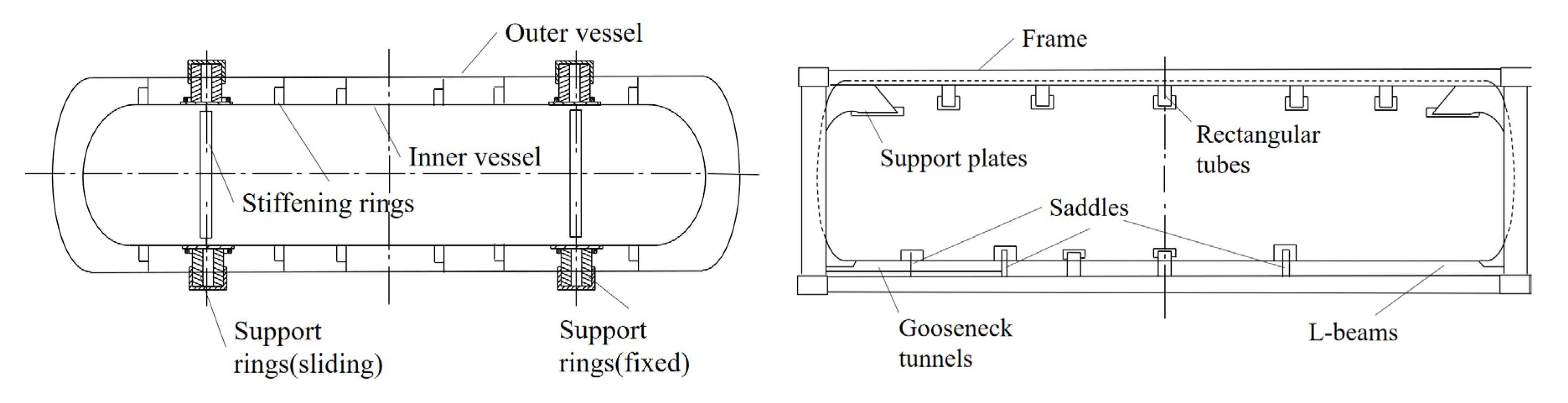
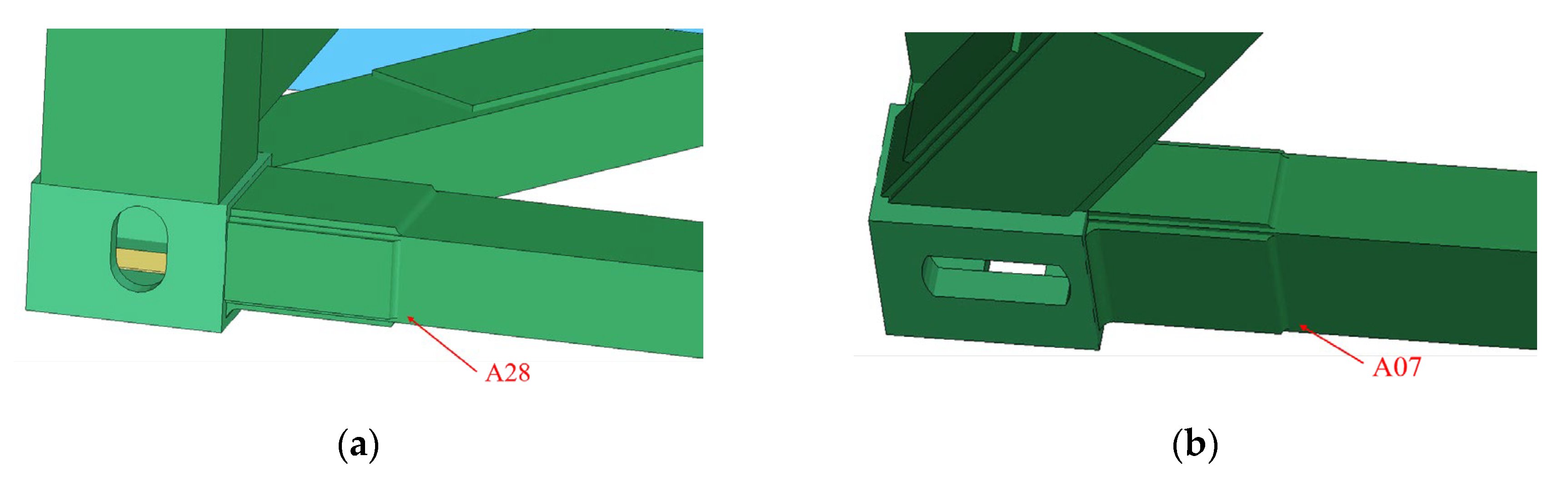
2.1. Structure of the Studied Tank Container

As shown in Figure 1, the inner and outer vessels, eight support rings, and frame make up the majority of the tank container. Eight support rings link the inner vessel (which holds the LNG) with the outer vessel, and the jacket is vacuumed to stop heat transmission. The frame’s dimensions are 12,192 mm × 2438 mm × 2591 mm (L × W × H), and the volume is 45.75 m³ with a 2425 mm outer vessel diameter.

Table 1. Main design parameters of the tank container.

Item	Value	Item	Value
Specified filling rate	90%	Material of the 8 support rings	GFRP
Design pressure of the inner vessel	0.6 MPa	Material of the inner vessel	S30408 (solution treatment)
Design temperature of the inner vessel	−196 °C	Material of the outer vessel	16MnDR (normalizing)
Design pressure of the jacket	−0.1 MPa	Material of the frame	Q450NQR1 (normalizing)
Design temperature of the jacket	50 °C	Corrosion allowance	0

lists the main design parameters of the tank container.

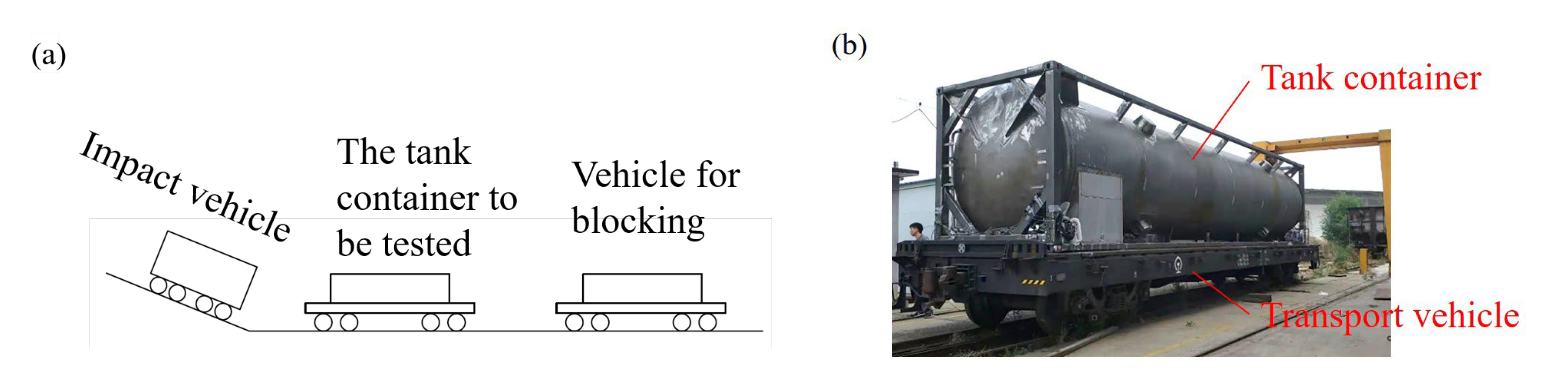
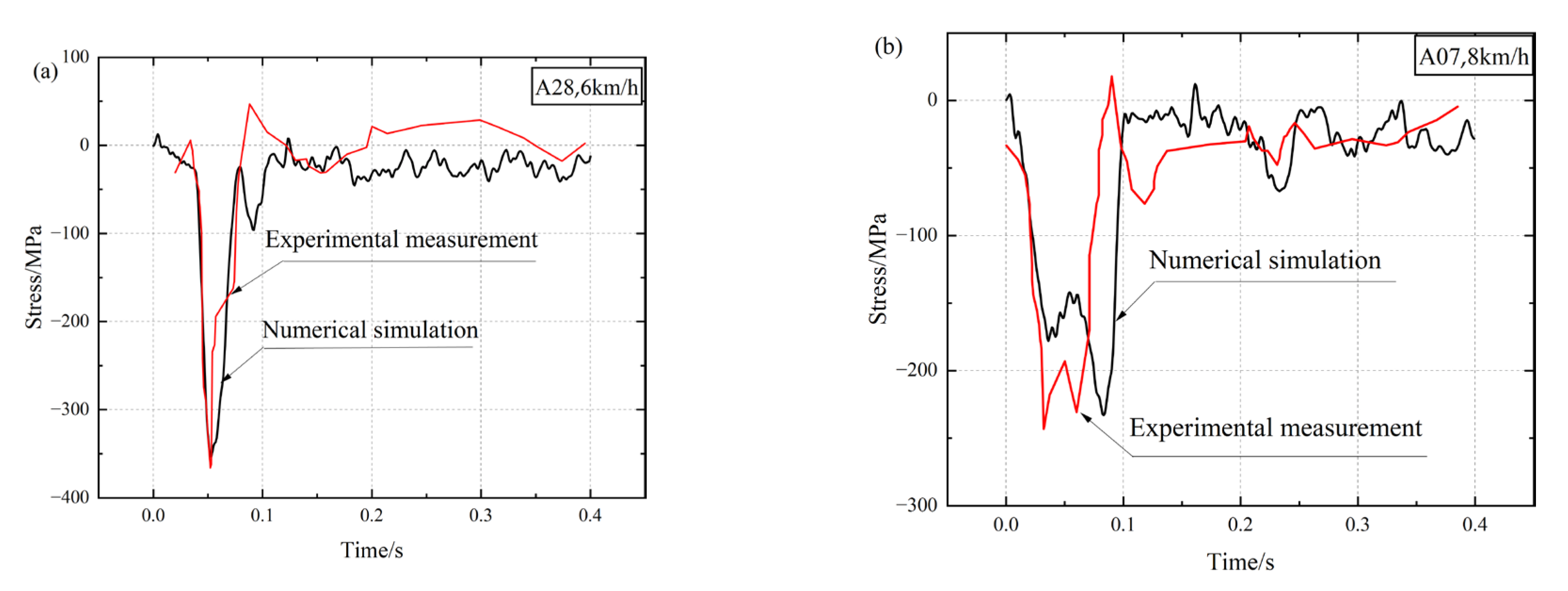
2.2. Impact Strength Test

The impact strength test was conducted in accordance with the Chinese standard TB/T1335-1996 Strength design and test certification specification for railway vehicle to determine whether the frame meets with the strength requirements. Water, foam, and rigid fixed supports were used as the filling medium, where the foam and rigid fixed supports were used to guarantee that the center of gravity of water was consistent with that of LNG of the same mass. The impact vehicle with MT-2 buffers slid down the hill and then hit the stationary, non-braking transport vehicle with the tank container for the test and MT-2 buffers. The impact vehicle was driven three times at each of the following velocities: 4 km/h, 5 km/h, 6 km/h, 7 km/h, and 8 km/h. The twist lock fixed to the transport vehicle then collided with the corner fittings of the tank container after the impact vehicle collided with the transport vehicle. The two vehicles eventually traveled in the direction of the rail after being linked by buffers. The impact test scheme and the field test are shown in Figure 2.

To measure stress, several strain gauges were installed on the tank container, particularly on the frame. When the impact vehicle’s initial velocity is 6.1 km/h, it is discovered that measuring point A28 on the longitudinal beam, near the corner fitting of the impact side, as shown in Figure 3a, has the largest compressive stress, with a maximum value of −366.3 MPa and a direction parallel to the impact direction. The variation in the stress at A28 over time is seen in Figure 3b. It can be seen that the impact has a significant effect on the frame, which lead to a peak compressive stress at A28. The impact vehicle’s collision effect is continually weakened as a result of the continuous energy consumption of MT-2 buffers, and the stress fluctuation at A28 decreases gradually.

3. Numerical Simulations

The finite element method was employed to simulate the above impact test using the explicit dynamic software LS-DYNA (MPP, R10.1.0).

3.1. Basic Algorithm

For Eulerian formulation, the Eulerian mesh node changes its position during one computational time step (mesh deforms) because of the loading. After the time step the analysis stops and the following two approximations are performed:

(1) Mesh smoothing: all the nodes of the Eulerian mesh, that have been displaced due to loading, are, moved to their original position;

(2) Advection: the internal variables (stresses, flow fields, velocity field) for all the nodes that have been moved are recomputed (interpolated) so that they have the same spatial distribution as before the mesh smoothing. In this way the mesh smoothing does not affect the internal variable distribution.

The described procedure is being repeated for each time step of the analysis. The ALE solving procedure is similar to Eulerian procedure. The only difference is the mesh smoothing. In the Eulerian formulation the nodes are moved back to their original positions, while in the ALE formulation the positions of the moved nodes are calculated according to the average distance to the neighboring nodes, meaning that the Eulerian mesh is movable and deformable.

The Null model algorithm was used to explain the fluid’s flow properties, while the control equations of the ALE were used to represent the fluid. The related Gruesien equation of state is further attached for resolution. The following is the Gruesien equation of state:

$$p=\frac{{\rho }_0{C}^2\mu \left[1+(1-\frac{{\gamma }_0}{2})\mu -\frac{a}{2}{\mu }^2\right]}{{\left[1-(S_1-1)\mu -S_2\frac{{\mu }^2}{\mu +1}-S_3\frac{{\mu }^3}{{(\mu +1)}^2}\right]}^2}+({\gamma }_0+a\mu )E$$

(1)

where C is the intercept of the ${\mu }_s$ (shock wave velocity)-${\mu }_p$ (particle velocity) curve (in velocity units); E is internal energy per unit volume; S₁, S₂, and S₃ are the unitless coefficients of the slope of the curve; ${\gamma }_0$ is the unitless Gruneisen coefficient; a is the unitless, first order volume correction to ${\gamma }_0$; and,

$$\mu =\frac{\rho }{{\rho }_0}-1$$

(2)

In general, the compressibility of fluid can be ignored, that is, $\rho \approx {\rho }_0$ is constant. Therefore, Equation (1) is simplified as:

$$p={\gamma }_{0}E$$

(3)

where the relationship of ${\gamma }_0$ with volume expansion coefficient $\alpha$, specific heat capacity $c_V$, density $\rho$ and isothermal compression coefficient $k_T$ is:

$${\gamma }_0=\frac{\alpha }{\rho c_V{k}_T}$$

(4)

The fluid structure interaction was realized by the penalty function method. According to the relative displacement, node forces are applied to the structure and the fluid, as shown in Figure 4, when the fluid particle passes through the structural element. Volume Fraction Initialization (VFI) was used to establish the boundary of the initial fluid material.

3.2. Material Model

Figure 5 shows the nominal stress-nominal strain curve for the Q450NQR1, 16MnDR, and S30408 materials.

$$S=(1+\epsilon )\sigma$$

(5)

$$e=\ln (1+\epsilon )$$

(6)

where $\sigma$ is nominal stress; $\epsilon$ is nominal strain; S is true stress; e is true strain. The true stress-strain curve is obtained by transforming the nominal stress-strain curve using Equations (5) and (6). For the yielding phase, the discontinuity of the yielding process is eliminated by selecting specific data points after the transformation [26].

Table 2. More structural material properties.

Item	Density (t/mm3)	Elastic Modulus (MPa)	Poisson’s Ratio
Impact vehicle	0.115 × 10−4	0.201 × 106	0.3
Transport vehicle	0.295 × 10−8	0.201 × 106	0.3
Twist lock	0.785 × 10−8	0.201 × 106	0.3
Corner fitting	0.785 × 10−8	0.201 × 106	0.3
GFRP	0.185 × 10−8	0.720 × 105	0.26

lists more structural material properties.

Table 3. Material properties of LNG.

Item	Value	Item	Value
Temperature (°C)	−161.87	$c_V$ (J/kg·k)	2056.3
Pressure (MPa)	0.1	$k_T$ (1/Pa)	2.22 × 10−9
Density (kg/m3)	460	$\alpha$ (1/K)	0.00346
Sound velocity (m/s)	1341.3	${\gamma }_0$	1.648
Viscosity (MPa·s)	0.118 × 10−9

lists the material properties of LNG with data referencing Refprop, a specialist program for cryogenic physical properties. The force-displacement curve was given to simulate the mechanical performance of the buffer using the experimental data [28]. The MT-2 buffer is characterized by a non-linear increase in force with increasing compression distance during loading, and very little during unloading, as shown in Figure 6.

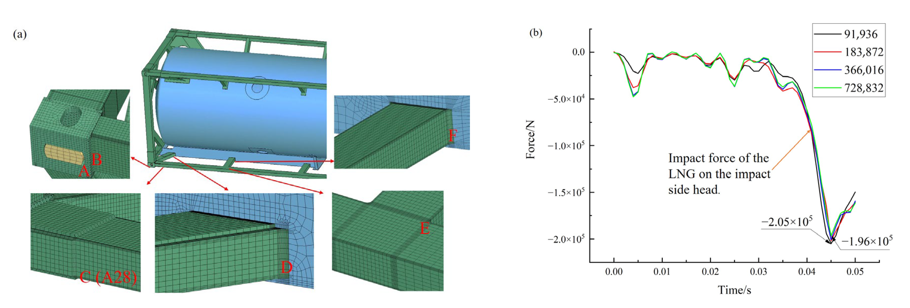
3.3. Modeling and Meshing

The impact vehicle and the transport vehicle were simplified to rigid cubes. The twist lock was fixed to the transport vehicle. The interface between LNG and containers was realized by the penalty function method. The geometry was modeled using LS-DYNA and Ansys software as shown in Figure 7.

Table 4. Mass of each model component.

Item	Impact Vehicle	Transport Vehicle	Tank Container	LNG (90%)
Mass (t)	92.0	23.0	12.9	18.9

lists the mass of each model component.

The buffer was meshed using Spring elements (Combi165, 2 nodes), while other components were meshed using solid elements (Solid164, 8 nodes) with sweep method. The ELFORM = −1 and ELFORM = 11 algorithms were assigned to solids and fluids element, respectively. Figure 8 shows the mesh model. There are 2,516,583 nodes and 1,954,231 elements that make up the tank container model. The fluid domain contains a total of 577,304 elements.

3.4. Loading and Boundary Condition

The weight of the tank container and the LNG, as well as the internal and external pressure (both 0.1 MPa), are all included in the load. Boundary conditions were set as follows. (1) The impact and transport vehicle traveled along the rail only, constraining the other directional translational degrees of freedom. (2) Friction contact was used with a friction coefficient of 0.15 between the corner fitting and the transport vehicle as well as between the support rings and vessels. The corner fitting and twist lock utilized automatic surface-to-surface contact. The common node method was used for the other structures. (3) The twist lock only established contact with the impact side corner fittings. The moment when the transport vehicle and the impact vehicle just collided is set to zero moment. Different initial velocities were applied to the impact vehicle, and there are differences in the impact direction initial clearance between the corner fitting and twist lock.

3.5. Model Verification

Take the initial velocity of 8 km/h and initial clearance of 6 mm as an example to verify the independence of load step and mesh, as shown in Figure 9 and Figure 10. Under different load steps, the maximum impact force at A (shown in Figure 10) and the force of LNG on the impact side head changed by 1.6% and 3.0%, respectively, as shown in Figure 9. Taking into account the mass change, the final load step was decided to be 1.89 × 10⁻⁷. In Figure 10, when the number of meshes was doubled, the maximum impact force at A changed by 2%, the axial stress at C (i.e., A28) changed by 4.2%, and the change of maximum Mises stress at other locations was within 0.2%. Additionally, the maximum LNG force changed by 4.6% when the number of fluid meshes in the contact region between the fluid domain and the tank container (part of the entire fluid domain) was refined from 91,936 to 728,832. After the verification, both the final load step and mesh were decided.

Only the inner vessel finite element model was built and filled with 50% of the volume of LNG, constraining all of the translational degrees of freedom of the outer surface of the inner vessel, in order to verify the reasonableness of the fluid-solid coupling contact parameters. When the theoretical value of the axial force of LNG on the head is compared to the simulation, the error is only discovered to be 2.2%. After the verification, the contact parameters were decided. The following formula was used to calculate the theoretical value:

$$F^{″}={\displaystyle \int pds}$$

(7)

where p is hydrostatic pressure; s is area.

The finite element model’s A28 and A07 locations are shown in Figure 11. Figure 12 shows the comparison between the experimental value and the simulated value of A28 and A07. It is found that the simulated value well agrees with the experimental one in stress variation trend, indicating that the finite element model is reasonable.

4. Results and Discussion

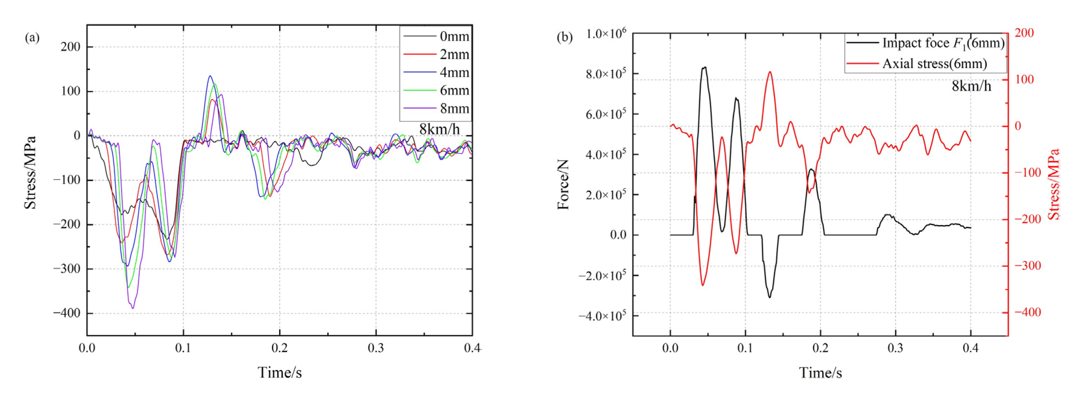
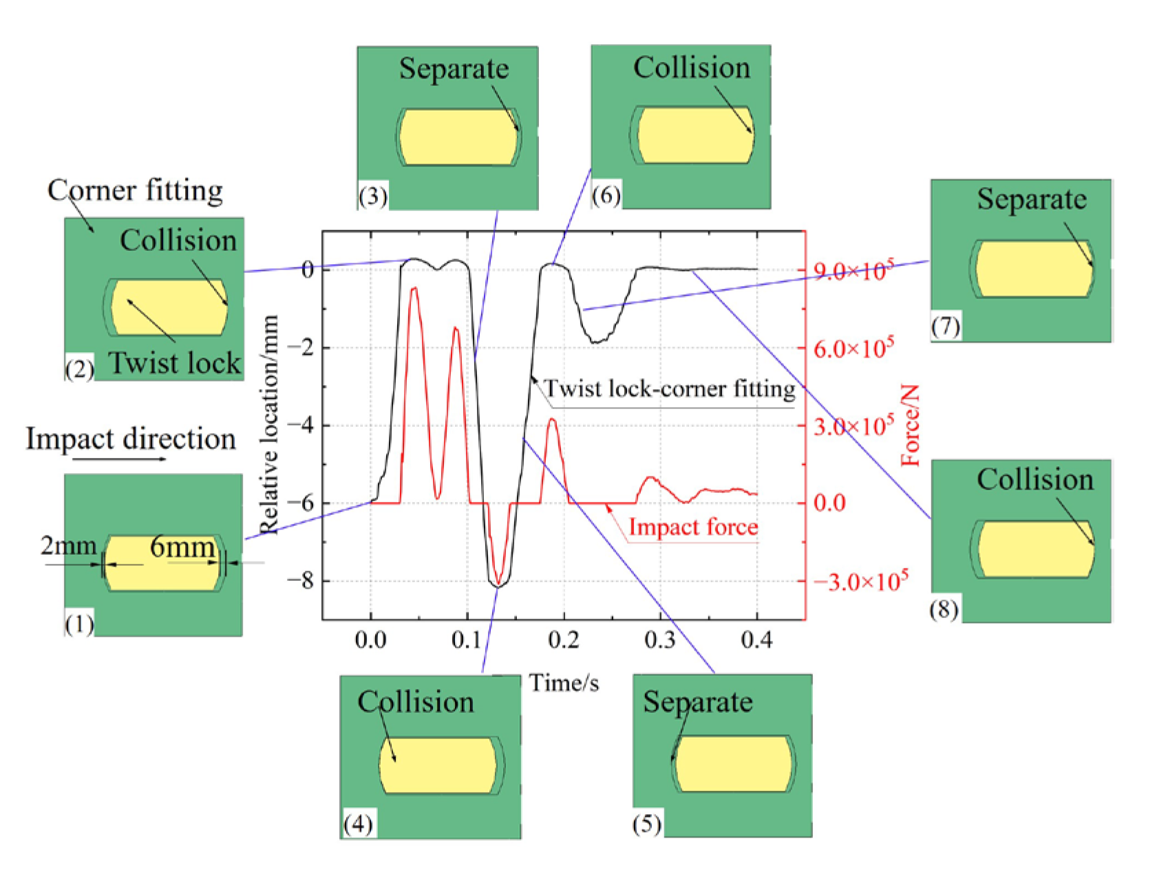
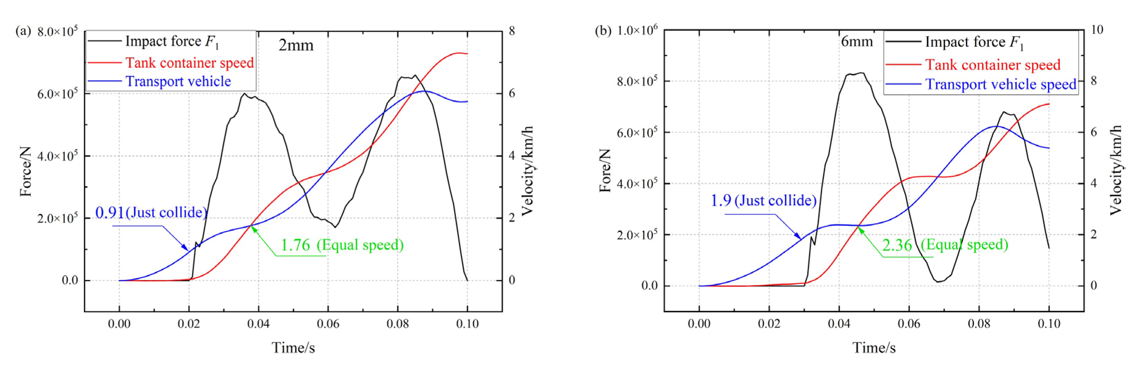
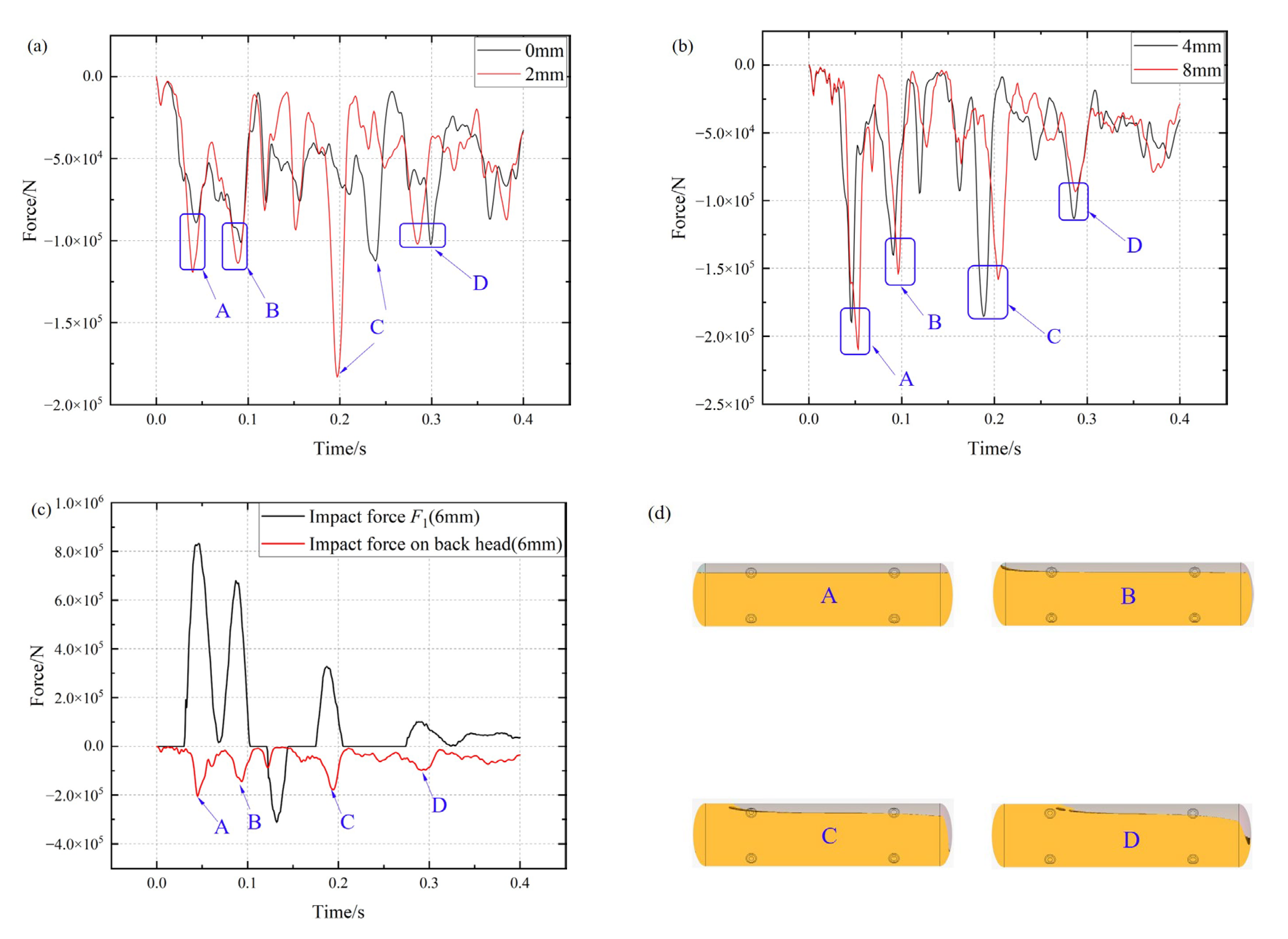
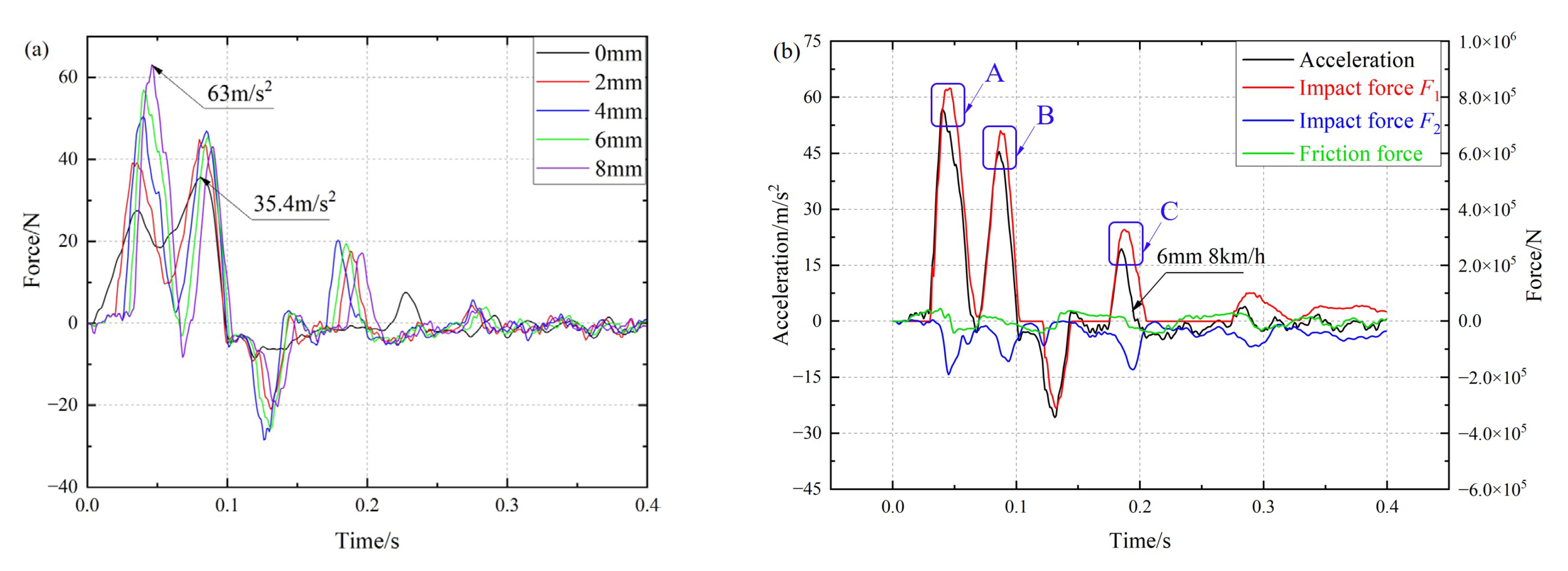
In this part, further simulation results were analyzed and discussed. The direction of the force involved in this section was along the impact direction, that is, along the rail transportation direction. The force was set to be positive in the direction of impact and negative in the opposite direction.

4.1. Impact Force

There are two kinds of impact forces: the first is the force of the twist lock on the corner fitting (F₁), and the second is the force of the LNG on the inner vessel (F₂). Figure 13 shows the variation in F₁ over time at different initial velocities and initial clearance. As can be seen, when the initial velocity is 8 km/h, the twist lock repeatedly impacts the corner fitting at each initial clearance, producing several peak forces, with the positive peak values being significantly greater than the negative peak values. The maximum of F₁ in direct relation to the initial clearance, increasing from 5.46 × 10⁵ N at 0 mm to 9.41 × 10⁵ N at 8 mm. However, its appearance time gradually moves from the second peak to the first peak. In addition, when the initial clearance is 8 mm, the magnitude and number of the peak of F₁ vary at different initial velocities. The F₁ significantly affects the axial stress at A07, which is shown in Figure 14 that when the force increases or decreases, the stress changes in magnitude accordingly.

Figure 15 shows the relationship between the F₁ and the relative location between the twist lock and the corner fitting. When the relative locations are between −8 and 0 mm, separation occurs, and when they are outside of that range, collision happens.

As can be seen from Figure 16, when the initial velocity is 8 km/h, the different initial clearance led to different velocities when the transport vehicle just collides with the corner fitting, which in turn affects the different magnitudes of the equal velocities and ultimately causes the different magnitudes of the first peak of F₁.

When the initial velocity is 8 km/h, Figure 17 shows the variation of the LNG impact force with time on the impact side head (back head) at different initial clearance. It can be seen that the back head is repeatedly impacted by the LNG at each initial clearance, resulting in multiple peak forces (such as A–D), and the maximum increases with the increase in initial clearance from −1.12 × 10⁵ N at 0 mm to −2.10 × 10⁵ N at 8 mm. In fact, the variation in LNG impact force is brought on by the F₁. However, although the F₁ changes sharply between positive and negative, the LNG impact force must remain negative. As in magnitude, the former is much larger than the latter. Figure 17d shows the variation in LNG free surface at different peak impact force times (split along the longitudinal symmetry plane). LNG separates from the front head and upwells along the back head as a result of inertia. LNG starts to surge along the axial direction of the tank container and upwell along the front head when it reaches the top of the inner vessel.

When the initial velocity is 8 km/h, Figure 18 shows the variation of the tank container axial acceleration at the mass center over time at different initial clearance. The maximum acceleration in direct relation to the initial clearance, from 35.4 m/s² at 0 mm to 63 m/s² at 8 mm. It is noted that the maximum acceleration is greater than 4g inertial acceleration specified in the Chinese standard NB/T 47059-2017 Tank containers for refrigerated liquefied gas for the design of tank containers, which means if assessed by the impact, the specifications of the standard are not conservative. In addition, as observed at locations A, B, and C in the Figure 18b, the acceleration has started to decrease before the peak value of F₁ as F₂ gradually approaches to the peak value.

The average pressure $p_{av}$ brought on by the LNG impact force on the back head is:

$$p_{av}=\frac{F_{\max }}{\pi r^2}$$

(8)

where F_max is the maximum LNG impact force; r is the inner radius of the inner vessel.

The static inertial force $F^{\prime }$ is:

$$F^{\prime }=ma$$

(9)

where m is LNG mass; a is the inertial acceleration. $F^{″}$ is calculated as 1.42 × 10⁴ N when the LNG filling percentage is 90%.

Table 5. The results of the calculation of each variable (8 km/h).

Clearance (mm)	Acceleration (m/s2)	Fmax (N)	${\mathit{p}}_{\mathit{a}\mathit{v}}$(MPa)	${\mathit{F}}^{\prime }$(N)	$\frac{{\mathit{F}}_{\mathbf{max}}}{{\mathit{F}}^{\prime }}$	$\frac{{\mathit{F}}_{\mathbf{max}}}{{\mathit{F}}^{″}}$
0	35.4	1.12 × 105	0.028	6.69 × 105	0.167	7.887
2	43.9	1.83 × 105	0.046	8.29 × 105	0.221	12.887
4	50.5	1.90 × 105	0.048	9.54 × 105	0.199	13.380
6	56.9	2.05 × 105	0.052	1.07 × 106	0.192	14.437
8	63.1	2.10 × 105	0.053	1.19 × 106	0.177	14.789

lists the results of the calculation of each variable at initial velocity of 8 km/h.

The data show that the largest average pressure is 0.053 MPa, or 8.83% of the 0.6 MPa design pressure. The inner vessel should be designed with a thickness allowance to account for the influence of LNG impact force. When the initial velocity is 8 km/h, the maximum LNG impact force on the back head is much more than the hydrostatic force, and the ratio of the maximum to the static inertia force at each clearance is less than 0.23, which means that the calculation method of LNG static inertia force is conservative.

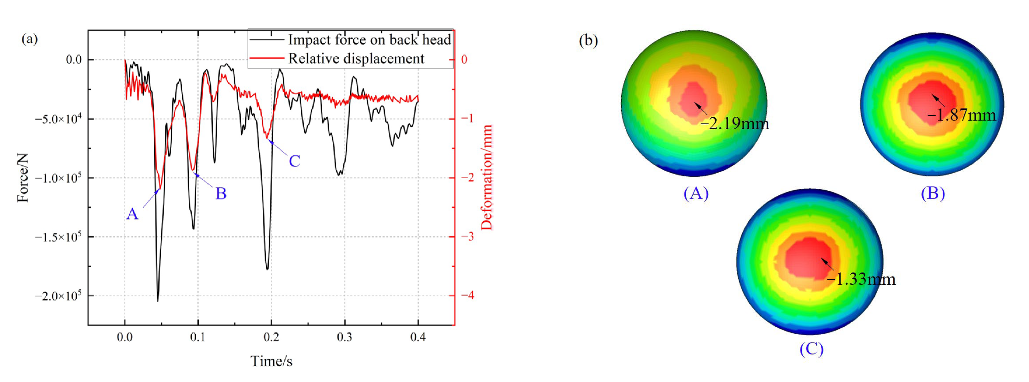
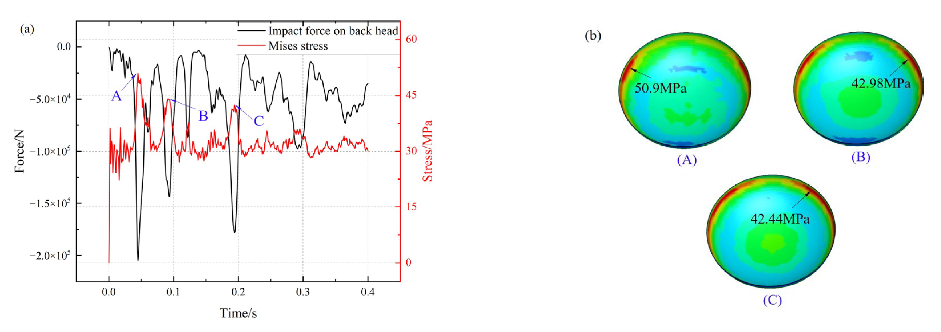
4.2. Influence of LNG Impact Force on Back Head

Figure 19 shows the variation of the back head maximum relative axial displacement over time (relative to the tank container axial displacement at the mass center) at the initial velocity of 8 km/h and the initial clearance of 6 mm. The maximum absolute value, 2.19 mm, occurs at the first peak moment of the impact force, and there is a one-to-one relationship between the peak impact force and the peak displacement, as does the maximum Mises stress in Figure 20. The maximum value, 50.9 MPa, occurs at the first peak moment of the impact force.

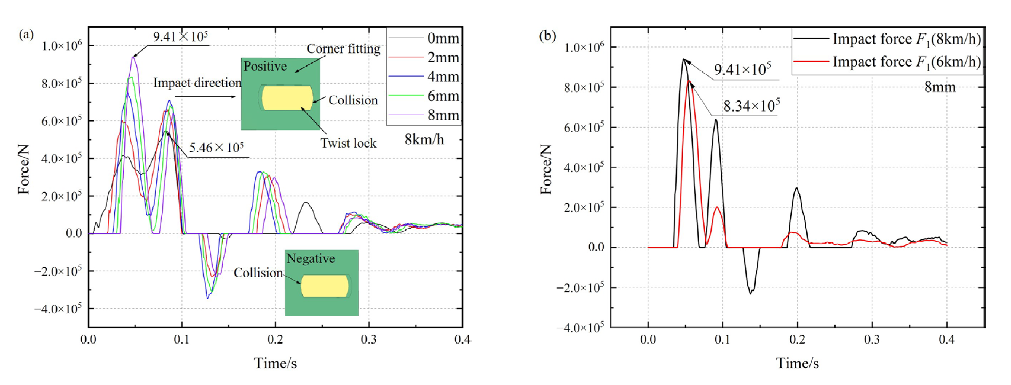
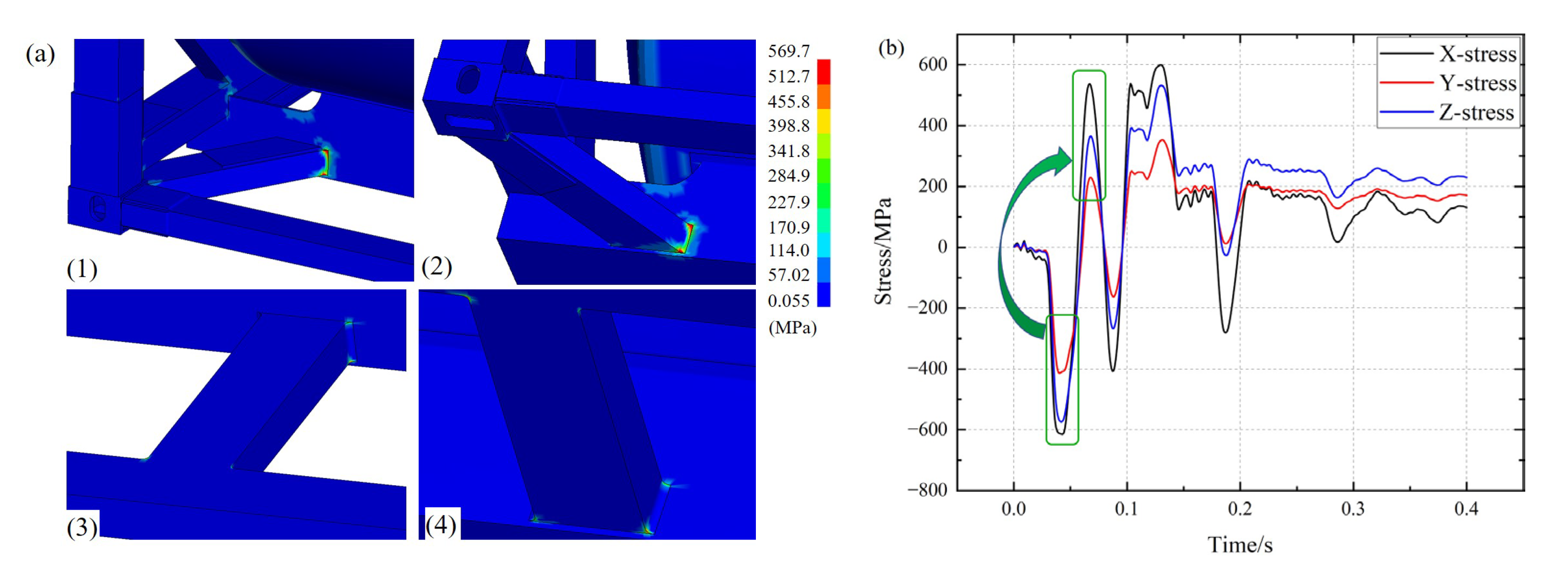
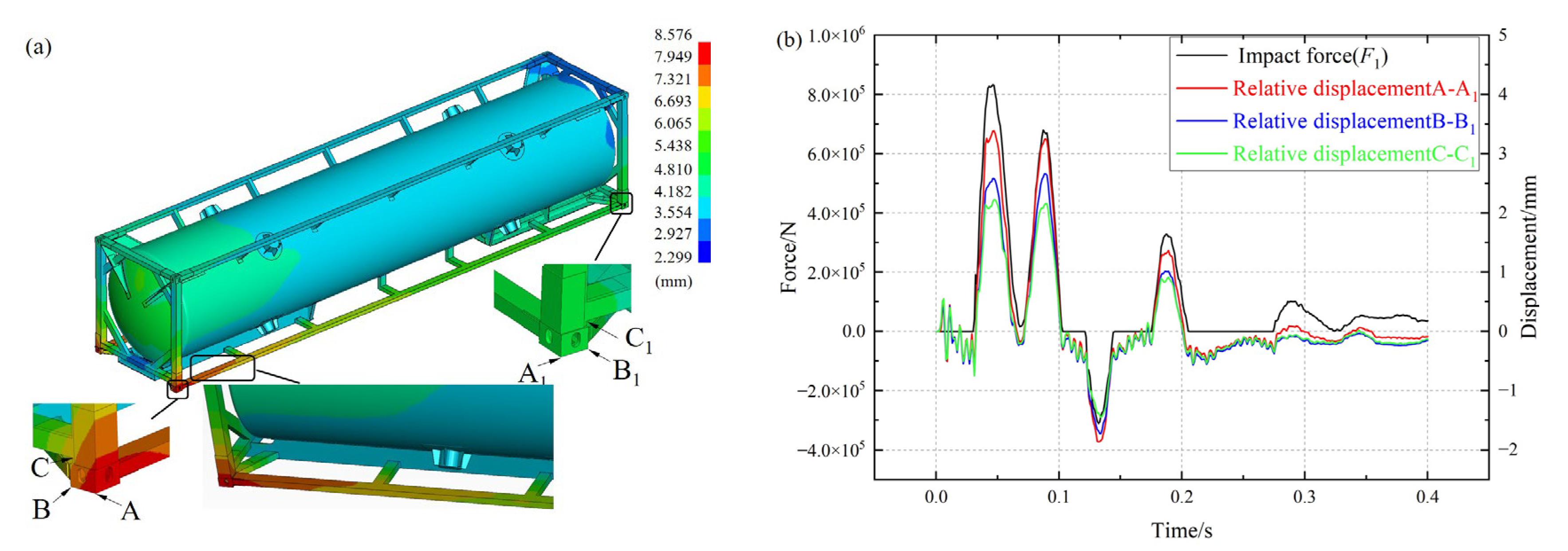
4.3. Influence of Impact Force F1 on Frame

Figure 21 shows the variation of the maximum Mises stress of the frame over time. It is clear that the maximum Mises stress has been significantly affected as a result of the impact force F₁. A, B, C, and D are the four stages that it could be divided into.

• At stage A, there is no F₁. Gravity has a significant role in determining the frame Mises stress, which is in the elastic range.
• Multiple impacts in stage B produce multiple stress peaks exceeding the yield strength (450 MPa). Peak value 1 is produced by the F₁ reaching its first peak value, and as can be seen in the Figure 22, there are many locations with high stress. With the exception of the chamfer, where residual stress causes high stress and a change in the stress state from compression to tension, as shown in Figure 23, the stress in other locations is low at peak value 2 in compared to the first peak. Comparable to peak values 1 and 2, peak value 3 and 4 have similar characteristics.

Figure 24 shows the distribution at the peak value 5, which is produced by the negative peak impact force. The negative impact force intensifies the tensile stress state at the chamfer.

3.

Although stage C do not have F₁, the maximum Mises stress is larger than the maximum Mises stress at stage A because of the residual stress at the chamfer. Stage D’s F₁ is low and has little effect on the stress distribution.

Figure 25 shows the axial displacement of the frame and outer vessel at the first peak of F₁. It is clear that the frame maximum axial displacement occurs at the corner fitting on the impact side and then gradually decreases in both the longitudinal and transverse directions. The relative deformation of the A-A₁, B-B₁, and C-C₁ varies in accordance with the F₁ alternating positive and negative variations. At the first peak of F₁, there is a 3.39 mm maximum relative deformation.

5. Conclusions

By performing the experiments and numerical simulations, impact process of a large LNG tank container for trains was investigated in this study. Conclusions are obtained as follows:

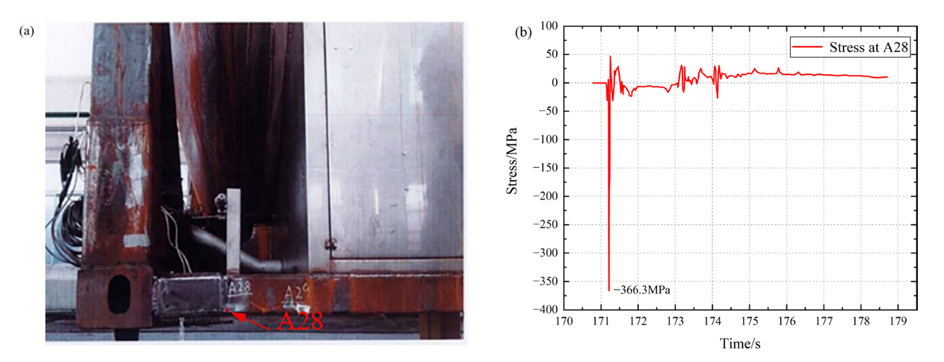
• The impact process of a large LNG tank container for trains was conducted experimentally and stresses on the container especially on the frame were measured with time. For the initial velocity of 6.1 km/h, the maximum compressive stress is −366.3 MPa occurring on the longitudinal beam near the impact side corner fittings.
• The impact force produced by the transport vehicle is influenced by both the initial clearance and initial velocity, i.e., its maximum value increases with the clearance or velocity, which in turn directly affects the LNG impact force on the head, the tank container axial acceleration at the mass center and the frame deformation and stress distribution. This result is valuable for the design of the corner fittings and frames of the container.
• The largest average pressure brought on by the LNG impact force is 0.053 MPa, or 8.83% of the 0.6 MPa design pressure, so the inner vessel should be designed with a thickness allowance. When the initial velocity is 8 km/h, the ratio of the maximum LNG impact force on the back head to the static inertia force at each clearance is less than 0.23, which means that the calculation method of LNG static inertia force is conservative. This result may be helpful for the design of the thickness of container.
• When the initial velocity is 8 km/h and the initial clearance is 8 mm, the maximum axial acceleration of the tank container is 63 m/s², greater than 4g inertial acceleration specified in the container design standard, meaning if assessed by the impact, the specifications of the standard are not conservative. This conclusion may provide reference for the editing or revision of the container design standard.

References

1. Goudarzi, M.A.; Sabbagh-Yazdi, S.R.; Marx, W. Investigation of sloshing damping in baffled rectangular tanks subjected to the dynamic excitation. Bull. Earthq. Eng. 2009, 8, 1055–1072. [Google Scholar] [CrossRef]
2. Akyildiz, H.; Uenal, N.E. Sloshing in a three-dimensional rectangular tank: Numerical simulation and experimental validation. Ocean. Eng. 2006, 33, 2135–2149. [Google Scholar] [CrossRef]
3. Anghileri, M.; Castelletti, L.; Tirelli, M. Fluid–structure interaction of water filled tanks during the impact with the ground. Int. J. Impact Eng. 2005, 31, 235–254. [Google Scholar] [CrossRef]
4. Zhang, A.N.; Suzuki, K. A comparative study of numerical simulations for fluid–structure interaction of liquid-filled tank during ship collision. Ocean. Eng. 2007, 34, 645–652. [Google Scholar] [CrossRef]
5. Aquelet, N.; Souli, M.; Gabrys, J.; Olovson, L. A new ALE formualtion for sloshing analysis. Struct. Eng. Mech. 2003, 16, 423–440. [Google Scholar] [CrossRef] [Green Version]
6. Nasar, T.; Sannasiraj, S.A.; Sundar, V. Experimental study of liquid sloshing dynamics in a barge carrying tank. Fluid Dyn. Res. 2008, 40, 427. [Google Scholar] [CrossRef]
7. Liu, D.M.; Lin, P.Z. A numerical study of three-dimensional liquid sloshing in tanks. J. Comput. Phys. 2008, 227, 3921–3939. [Google Scholar] [CrossRef]
8. Kang, N.; Liu, K. Influence of baffle position on liquid sloshing, during braking and turning of a tank truck. J. Zhejiang Univ. A 2010, 11, 317–324. [Google Scholar] [CrossRef]
9. Cao, Y.; Jin, X.L. Dynamic response of flexible container during the impact with the ground. Int. J. Impact Eng. 2010, 37, 999–1007. [Google Scholar] [CrossRef]
10. Ibrahim, R.A. Assessment of breaking waves and liquid sloshing impact. Nonlinear Dyn. 2020, 100, 1837–1925. [Google Scholar] [CrossRef]
11. Jung, J.H.; Yoon, H.S.; Lee, C.Y.; Shin, S.C. Effect of the vertical baffle height on the liquid sloshing in a three-dimensional rectangular tank. Ocean Eng. 2012, 44, 79–89. [Google Scholar] [CrossRef]
12. Zhang, Z.L.; Khalid, M.S.U.; Long, T.; Chang, J.Z.; Liu, M.B. Investigations on sloshing mitigation using elastic baffles by coupling smoothed finite element method and decoupled finite particle method. J. Fluids Struct. 2020, 94, 102942. [Google Scholar] [CrossRef]
13. Sauer, M. Simulation of high velocity impact in fluid-filled containers using finite elements with adaptive coupling to smoothed particle hydrodynamics. Int. J. Impact Eng. 2011, 38, 511–520. [Google Scholar] [CrossRef]
14. Pal, N.C.; Bhattacharyya, S.; Sinha, P.K. Non-linear coupled slosh dynamics of liquid-filled laminated composite containers: A two dimensional finite element approach. J. Sound Vib. 2003, 261, 729–749. [Google Scholar] [CrossRef]
15. Reed, P.E.; Breedveld, G.; Lim, B.C. Simulation of the drop impact test for moulded thermoplastic containers. Int. J. Impact Eng. 2000, 24, 133–153. [Google Scholar] [CrossRef]
16. Wang, W.Y.; Peng, Y.; Zhang, Q.; Ren, L.; Jiang, Y. Sloshing of liquid in partially liquid filled toroidal tank with various baffles under lateral excitation. Ocean Eng. 2017, 146, 434–456. [Google Scholar] [CrossRef]
17. Tiernan, S.; Fahy, M. Dynamic FEA modelling of ISO tank containers. J. Mater. Process. Technol. 2002, 124, 126–132. [Google Scholar] [CrossRef]
18. Dai, L.; Xu, L.; Setiawan, B. A new non-linear approach to analysing the dynamic behaviour of tank vehicles subjected to liquid sloshing. Proc. Inst. Mech. Eng. Part K J. Multi-body Dyn. 2005, 219, 75–86. [Google Scholar] [CrossRef]
19. Li, J.G.; Hamamoto, Y.; Liu, Y.; Zhang, X. Sloshing impact simulation with material point method and its experimental validations. Comput. Fluids 2014, 103, 86–99. [Google Scholar] [CrossRef]
20. Wu, W.F.; Zhen, C.W.; Lu, J.S.; Tu, J.Y.; Zhang, J.W.; Yang, Y.B.; Zhu, K.B.; Duan, J.X. Experimental study on characteristic of sloshing impact load in elastic tank with low and partial filling under rolling coupled pitching. Int. J. Nav. Arch. Ocean Eng. 2020, 12, 178–183. [Google Scholar] [CrossRef]
21. Kim, Y. Numerical simulation of sloshing flows with impact load. Appl. Ocean Res. 2001, 23, 53–62. [Google Scholar] [CrossRef]
22. Bendarma, A.; Jankowiak, T.; Rusinek, A.; Lodygowski, T.; Klosak, M. Perforation Tests of Aluminum Alloy Specimens for a Wide Range of Temperatures Using High-Performance Thermal Chamber-Experimental and Numerical Analysis. In IOP Conference Series: Materials Science and Engineering; IOP Publishing: Bristol, UK, 2019; Volume 491, p. 012027. [Google Scholar]
23. Kpenyigba, K.M.; Jankowiak, T.; Rusinek, A.; Pesci, R. Influence of projectile shape on dynamic behavior of steel sheet subjected to impact and perforation. Thin-Walled Struct. 2013, 65, 93–104. [Google Scholar] [CrossRef] [Green Version]
24. Bendarma, A.; Jankowiak, T.; Łodygowski, T.; Rusinek, A.; Klósak, M. Experimental and numerical analysis of the aluminum alloy AW5005 behavior subjected to tension and perforation under dynamic loading. J. Theor. Appl. Mech. 2017, 55, 1219–1233. [Google Scholar] [CrossRef] [Green Version]
25. Song, T.T. Research on Q450NQR1 High Strength Sheet Metal forming Springback and Application of Shallow Drawing. Diploma Thesis, Shandong University, Jinan, China, 2011. [Google Scholar]
26. Pan, J.H.; Chen, Z.; Hong, Z.Y. A novel method to estimate the fracture toughness of pressure vessel ferritic steels in the ductile to brittle transition region using finite element analysis and Master Curve method. Int. J. Press. Vessel. Pip. 2019, 176, 103949. [Google Scholar] [CrossRef]
27. Han, Y. Study on Technique of Cold Stretched Austenitic Stainless Steel Pressure Vessle and Its Performance Evaluation in Typical Media Environment. Diploma Thesis, Hefei University of Technology, Hefei, China, 2012. [Google Scholar]
28. Mi, L. Research on Numerical Simulation of Impact Test on Railway Vehicles. Diploma Thesis, Beijing Jiaotong University, Beijing, China, 2014. [Google Scholar]
Figure 1. Schematic diagram of the tank container.
Applsci 13 01351 g001
Figure 2. The impact test: (a) scheme; (b) field tests.
Applsci 13 01351 g002
Figure 3. Measuring point A28: (a) location of A28; (b) the variation of stress at A28 over time.
Applsci 13 01351 g003
Figure 4. Lagrange-Eluerian coupling diagram.
Applsci 13 01351 g004
Figure 5. Nominal stress-nominal strain curve: (a) Q450NQR1 [25]; (b) 16MnDR [26]; (c) S30408 [27].
Applsci 13 01351 g005
Figure 6. The force-displacement curve of MT-2.
Applsci 13 01351 g006
Figure 7. Geometry of the impact vehicle and the transport vehicle created in LS-DYNA and Ansys.
Applsci 13 01351 g007
Figure 8. Mesh model: (a) structure, (b) ALE element (partial).
Applsci 13 01351 g008
Figure 9. Load step independence verification: (a) impact force of the transport vehicle on the tank container, (b) impact force of the LNG on the impact side head.
Applsci 13 01351 g009
Figure 10. Mesh independence verification: (a) frame mesh, (b) fluid mesh in the contact region.
Applsci 13 01351 g010
Figure 11. Location of A28 and A07 in the finite element model: (a) A28; (b) A07.
Applsci 13 01351 g011
Figure 12. Comparison between experimental and simulated values: (a) A28 with the impact vehicle velocity of 6 km/h; (b) A07 with the impact vehicle velocity of 8 km/h.
Applsci 13 01351 g012
Figure 13. The variation in F1 over time: (a) at different initial clearance; (b) at different initial velocities.
Applsci 13 01351 g013
Figure 14. The variation of axial stress at A07: (a) at different initial clearance; (b) relationship with the F1.
Applsci 13 01351 g014
Figure 15. Relationship between the F1 and the relative location between the twist lock and corner fittings.
Applsci 13 01351 g015
Figure 16. Relationship between the F1 and the velocity of the transport vehicle and tank container (a) at 2 mm initial clearance; (b) at 6 mm initial clearance.
Applsci 13 01351 g016
Figure 17. The variation of LNG impact force: (a) at 0 and 2 mm initial clearance; (b) at 4 and 8 mm initial clearance; (c) relationship with the F1; (d) LNG free surface at peak impact force times.
Applsci 13 01351 g017
Figure 18. The variation of the tank container axial acceleration at the mass center over time: (a) at different initial clearance; (b) relationship with the F1, F2 and friction force between corner fittings and the transport vehicle.
Applsci 13 01351 g018
Figure 19. The variation of the back head maximum relative axial displacement over time: (a) relationship with the LNG impact force; (b) location of three peak displacements.
Applsci 13 01351 g019
Figure 20. The variation of the maximum Mises stress at the back head over time: (a) relationship with the LNG impact force; (b) location of three peak stresses.
Applsci 13 01351 g020
Figure 21. The variation of the maximum Mises stress of the frame over time.
Applsci 13 01351 g021
Figure 22. Stress distribution at peak value 1.
Applsci 13 01351 g022
Figure 23. Stress distribution at peak value 2: (a) location, (b) change of stress state in chamfer.
Applsci 13 01351 g023
Figure 24. Stress distribution at peak value 5: (a) location; (b) change of stress state in chamfer.
Applsci 13 01351 g024
Figure 25. The axial displacement of the frame and outer vessel: (a) at the first peak of F1, (b) relationship with the F1.
Applsci 13 01351 g025