Abstract
To solve the problem of the high cost of transient temperature simulation in the whole construction process of an asphalt-concrete core wall, a novel adaptive degree of freedom condensation algorithm for simulating transient temperature is proposed. This method establishes the judgment criterion of degree of freedom condensation based on the error estimator of mesh and the artificial energy added by degree of freedom condensation. In this method, the transformation matrix between the master and slave degrees of freedom is constructed based on the shape function interpolation relationship between the initial coarse mesh and the multi-level refined mesh. In the transient calculation process, this method can automatically identify the positions where temperature distribution and value are stable and condense the considered slave degrees of freedom to master degrees of freedom through the transformation matrix at any time to reduce the unnecessary degrees of freedom. In this paper, three numerical examples show that the proposed method can effectively reduce the cost of matrix factorization and the solving the equation in the finite element method at the cost of small precision loss in the long-term transient temperature simulation.
1. Introduction
Asphalt concrete is a kind of viscoelastic-plastic and environmentally friendly material that is widely used in road construction, general construction, water conservancy, and other engineering fields. In the field of water conservancy, asphalt concrete is generally used as the core wall of embankment dam to prevent seepage because it has the special characteristics of low permeability to ensure water tightness, high flexibility preventing cracking due to imposed embankment deformations, resistance to aging, and good self-healing capacity and resistance against erosion [1]. Because of these advantages, more and more rockfill dams use asphalt-concrete core walls as impermeable structures. Up to now, more than 200 asphalt-concrete core-wall dams have been built in the world, the most representative of which include Storglomvatn Dam in Norway [2], Finstertal Dam in Austria [3], and Yele Dam and Quxue Dam in China [4,5].
There have been many studies on the long-term health of concrete dams [6,7], but the service behavior of the asphalt-concrete core-wall dam is not clear. The asphalt-concrete core wall is the main impermeable structure, and its impermeable performance directly affects the health of the whole dam. The construction quality of the asphalt-concrete core wall is a key factor in achieving good impermeability. The poor quality of the construction can lead to construction defects such as cracks or holes in the core wall, which if not healed can lead to potential leakage paths affecting the impermeability of the core wall. Asphalt concrete is a viscoelastic-plastic material that is temperature-sensitive, and its mechanical properties and construction quality are temperature-dependent, so the temperature of the asphalt concrete needs to be controlled during construction [8,9]. If there is a long interval between the construction of the asphalt-concrete core-wall layers, the surface of the core-wall layers will cool to low temperature (especially in cold areas) and temperature cracks will easily appear between the layers which will create potential defects. However, if the interval between the construction of the asphalt-concrete core wall is short, the compaction of the asphalt concrete in a high temperature state will be poor and can lead to an uncompacted core wall, which can also result in holes or cracks. So, safeguarding the impermeability of asphalt-concrete core walls requires one to pay attention to the temperature changes in the asphalt-concrete core walls. Specifically, each layer of asphalt concrete needs to be paved and compacted at high temperatures until it cools and becomes hard. Only then will the latter layer be allowed to continue construction. From the point of view of heat transfer, the high temperature of the latter layer affects the temperature state of the previous layer. However, there are few research studies to simulate the temperature change of the asphalt-concrete core wall from the construction period to the operation period, and it is common to use a laboratory test to obtain mechanical parameters at a certain temperature to simulate the mechanical properties of the core wall, which will be difficult to guide and will guarantee the construction quality of the asphalt-concrete core wall from the perspective of numerical calculation. For this reason, to obtain the mechanical properties of the asphalt concrete at any location in the core wall during the construction period, it is necessary to simulate the temperature during the paving and cooling of the asphalt concrete. Moreover, a problem with simulating the paving and cooling of the asphalt-concrete core wall is that a layer of asphalt concrete is typically 20–25 cm [1,10], which is a large difference in scale compared to the tens to hundreds of meters of the whole core wall. If each layer were to be finely simulated during the construction period, its computational cost would increase significantly.
According to the construction and service features of the asphalt-concrete core wall, we can know that the core-wall temperature has the following two characteristics. Firstly, because the core wall is inside the dam and the rockfill material plays the role of thermal insulation, external temperature has less influence on the core-wall temperature, and eventually the core-wall temperature gradually tends to a stable interval. Secondly, the core-wall layers further away from the current construction layer do not have significant temperature fluctuations influenced by the construction layer. In summary, the location of the large temperature gradient in the core wall changes with the progress of construction and the temperature gradient tends to decline with time, that is, the distribution of the rapid temperature changes is local in space and time.
Considering the characteristics above, we find that the construction of asphalt-concrete core walls has a similar process to that of multi-layer deposition of materials in additive manufacturing, in which they have the same characteristics of temperature change. Therefore, the simulation method for multi-layer deposition is useful for the simulation of asphalt-concrete core walls. The finite element method is widely used in solving such problems due to its adaptability to irregular geometric computational regions, its ability to obtain reliable and convergent approximate solutions with refined mesh, and its efficiency at solving symmetric strip sparse arrays. There has been an amount of research into the thermal finite element simulation of multi-layer deposition of materials [11,12,13,14]. For thermal simulations of multi-layer deposition, at the beginning of the simulation, the corresponding element of the material that has not yet been deposited is set to a quiet state, and when a moving energy source is applied to the element, the element is switched to active. In comparison, the thermal simulation of the construction of asphalt concrete is simpler because there is no need to set up an external moving energy source. For the layers that have been constructed, the new layer is similar to a gradually cooling heat source with direct heat transfer through solid contact. Like the construction of asphalt-concrete core wall, in multi-layer deposition manufacturing of large parts, the analysis time increases with the number of nodes (or degrees of freedom) in the model [15]. Compared to the full meshes, the use of adaptive meshes at this time is effective at reducing the computational time. The most common method of adaptive mesh is to regenerate new elements in the geometry based on coarsening or refinement criterion according to the results of the current time step and then to map the results between refined and coarse meshes. The methods to reduce the size of the computation by building adaptive meshes include the layer-by-layer coarsening of the mesh based on layer distribution [15,16,17], the coarsening of the mesh based on user-defined classifications [18], the coarsening of the mesh based on localized conformal coarsening [19,20], and the coarsening of the mesh based on the hierarchy of refinement levels defined by an octree parental structure [21,22,23,24]. The advantages of this geometrically adaptive mesh are that it directly shows the changes in the model and highlights the locations that require attention, but the disadvantages are that an amount of element information needs to be handled. This information includes the complex relationships of parent and child element [21], the repositioning and recalculation of element nodes and Gaussian integration points [15,24], and the calculation of corresponding coefficient of interpolation [17]. Considering that most of the time in finite element method (FEM) calculations is spent in solving large systems of equations, the larger the system of equations, the longer the time required to solve them. It is well known that the size of the systems of equations is directly related to the number of degrees of freedom (DOFs), and it is clear that the DOFs are associated with the nodes. The geometrically adaptive mesh discussed earlier reduces the number of DOFs by reducing that of nodes. If the number of DOFs can be reduced directly, that is, the size of equations can be reduced from the algebraic point of view, even without changing the nodes, it is clear that the time to solve the equations can be reduced.
In computational mechanics, the DOF condensation method can reduce the number of DOFs in the stiffness matrix [25]. The method was first proposed by Guyan in 1965 and was named static condensation because it is only accurate for static problems [26]. Later, the method began to be extended to dynamic calculations [27,28,29]. DOF condensation methods are currently mostly used to analyze substructures where users focus on regions that have some characteristics, that is, substructuring analysis [30]. This eliminates some or all of the DOFs in other regions and then allows for the detailed analysis of the localized region (e.g., the simulation of large reinforced concrete structures with localized nonlinearities [31,32]). In fact, similarly, based on the error-control method, it is possible to eliminate some DOFs and obtain the satisfactory results with the analysis of the global region [33].
Considering that the temperature inside the core wall generally decreases and stabilizes from the construction period to the operational period, there will be no significant difference in temperature between the multiple core wall construction layers inside. In this case, an approximately accurate result can be calculated by eliminating some of the local DOFs and retaining only a small number of DOFs in the global region. Therefore, this paper proposes an adaptive DOF condensation method to automatically eliminate the temperature DOF of the core wall at a different time and then eventually achieve the reduction of the computational time and ensure the accuracy of the calculation results required.
In this paper, Section 2 provides the derivation process of the method proposed in this paper and introduces the corresponding coarsening criterion and the transformation matrix used. Three examples are used in Section 3. The first and second examples verify the efficiency and accuracy of the method for the calculation of the transient temperature field in the invariant and variable computational domains, respectively. Additionally, based on an engineering problem, the third example verifies the applicability of the method to simulate the temperature field in the construction process of asphalt-concrete core wall. Similar to the simulation of the transient temperature field during the construction period of asphalt-concrete core walls, usually such problems have large differences in structural spatial scales, long computational time domains, and high model-refinement requirements. Section 4 summarizes the cost advantages and limitations of the method proposed in this paper when solving this type of problem and also describes the possible directions for further improvement.
2. Methodology
The adaptive DOFs condensation method proposed in this paper derives the discretization form of the basic equation of the DOFs condensation for the transient heat-conduction problem, adaptively judges DOFs condensation based on the error estimator and coarsening criterion, and establishes the transformation matrix between the master and slave DOFs based on the interpolation relationship between the coarse mesh and the refined mesh. The method proposed in this paper is abbreviated as ADOF-FEM in the following sections.
2.1. DOFs Condensation of Transient Heat-Conduction Problem
Firstly, consider the basic form of the static equations:
The equation can be divided into two groups: the master DOFs, which will be retained, here denoted by the subscript m, and the slave DOFs, which will be removed, here denoted by the subscript s.
Define a transformation matrix
Substitute Equation (3) into Equation (1) and multiplying both sides of this equation by a matrix . It can be written in a similar form:
where:
Applying the Galerkin method for the transient equations subjected to appropriate boundary and initial conditions, the basic form of the transient heat conduction equations can be written as follows [34]:
where is the global heat capacitance matrix; is the global conductivity matrix, which contains the heat conduction matrix and the contribution matrix of heat flow boundary to heat conduction matrix; is the thermal force vector, which is contributed to by the heat flow boundary and the heat source; represents the temperature; and represents the derivative of temperature with respect to time.
As suggested by Guyan [26], the mass matrix in the basic form of the dynamic equations can be reduced through the transformation matrix given in Equation (3). Similarly, the temperature and the derivative of temperature with respect to time are assumed to have the same transformation relationship in the master and slave degrees of freedom:
Using the generalized Newmark method [35], the temperature and the derivative of the temperature with respect to time are as follows, respectively:
where, and n represent the time step; represents the time difference between time steps; is the Newmark parameter; and the parameter generally is 0.5 when using the implicit solution method.
2.2. Error Estimator
For heat-conduction problems, there are locations with large or small temperature gradients, the former of which require a refined mesh and the latter of which can use a coarse mesh. However, it is usually difficult to obtain the laws before calculation. Moreover, the temperature gradient changes over time for transient heat-conduction problems, and regions with a large temperature gradient may be smaller after a number of time steps. At this time, the initial refined mesh, which has a large number of DOFs, will have a large computational cost, so it is important to reduce the DOFs without affecting the computational accuracy too much.
In fact, it is necessary to obtain the global error of the whole computed domain before considering DOFs condensation. If the error exceeds the prespecified error limit, it is usually recommended that the mesh needs be refined to achieve a better calculation result, and conversely if the error is small the mesh can be coarsened. The error is calculated from the approximate solution of the computational mesh and the analytical solution of the partial differential equation, but the analytical solution of the practical engineering is usually not available (obviously, there is no need to perform a finite element calculation if the analytical solution has already been obtained). Therefore, an error estimator is needed to estimate the global error of the current calculation result.
Zienkiewicz and Zhu [36] first proposed a simple error estimator for the linear elastic static problem, and then Franca and Haghighi [37] derived an error estimator for heat-conduction problems that use the most commonly used energy norm and apply the boundary conditions results. It can be defined as
where T is the temperature calculation value and is the temperature exact value, respectively; k is the thermal conductivity coefficient; h is the convective heat-transfer coefficient; is the computational domain; and is the heat flow boundary.
Similarly, the exact energy norm considered to be a measure of the total heat dissipation in the whole domain can be calculated as
A relative error measure can be defined as
where is a prespecified error limit for the global relative error and the relative error is bounded by it.
Zienkiewicz and Zhu [36] use the smoothed values of stresses instead of the exact values to calculate the error norm. Similarly, Huang and Lewis [38] applied the smoothing procedure to heat-transfer problems. Using the smoothing procedure, the computation field in Equation (18) can be replaced with the smoothed values. The smoothed temperature gradient at any location within the element can be interpolated by the smoothed temperature gradient of the nodes and the shape functions. It can be calculated as:
where n is the number of nodes per element, are the shape functions, are the smoothed temperature gradient of the nodes, and are the values of the smoothed temperature gradient an any point in the element, respectively.
In the case of transient heat conduction, the precondition for mesh coarsening is not only that the error of a certain step is below the prespecified error limit but also to ensure that the error is below the tolerance value for a long time. Franca and Haghighi [37] proposed the variation of the error with respect to time to determine the trend of error over time, and to ensure that the mesh can be coarsened during this time. It can be calculated as
where is the error at the time ; is the error at the time t; and is a prespecified tolerance value for .
2.3. Mesh-Coarsening Criterion
The error estimator introduced in Section 2.2 quantifies the posterior error calculated in the computational domain based on the current mesh; if the mesh coarsening is carried out at this time, the difference values between the mesh before and after the coarsening is difficult to obtain in advance, so it is necessary to establish a mesh-coarsening criterion to ensure that the additional calculation error introduced by the coarsening process solves the problem or meets the engineering requirements.
Coarsening is actually the reverse of refinement, so the method of refinement should be introduced first. There are two main directions of refinement. The first refinement is the simple reduction of the subdivision size (h-refinement), and the second refinement uses the high-order shape functions (p-refinement). It is usually simple and natural for most engineers to use h-refinement, and the method proposed in this paper is also based on h-refinement.
If refinement improves computational accuracy, then coarsening as the reverse of refinement certainly adds additional errors that, in the form of energy, can be seen as artificial energy. This artificial energy can be quantified as [39]:
where and are the energy stored in the coarsened mesh and the original refined mesh, respectively. It is assumed that the mesh is unchanged before time and coarsening at time ; we can obtain that and are equal. So, the artificial energy added at time can be quantified as
where and are the difference of and between time and time , respectively.
The energy E stored in the domain is
where is the density of the material and is the specific heat capacity of the material; the unit of temperature needs to be convert to Kelvin, K.
And the difference of E between time and time is
Assuming that the mesh is unchanged before time and coarsening at time , the temperature at time has the following relationship:
The large difference in the energy stored in different time steps and different elements will make it difficult to compare the added artificial energy, so it is necessary to use the relative artificial energy as the coarsening criterion. The relative artificial energy can be written as
where is the maximum allowable relative artificial energy in the element in order to allow coarsening.
Consider a heat-conduction problem in which the temperature field changes gradually stabilize; a very small amount of the value of the relative artificial energy sometimes appears in the early time of the calculation, which leads to an incorrect judgment that the current step satisfies the coarsening criterion. In order to prevent an incorrect judgment, the other coarsening criterion is established as follows:
Based on the method of h-refinement, it is assumed that the initial computational mesh is formed by refining the initial coarse elements n times, and the initial coarse elements are defined as level 0, while all the elements formed by refining once are level 1, and so on, and the elements of the initial computational mesh are all level n.
When all of the higher-level elements (refined mesh) contained in a lower-level element (coarse mesh) meet the above two coarsening criteria at a certain time then the DOFs contained in the lower-level element are the master DOFs, and the others contained in the higher-level elements are all regarded as slave DOFs and reduced by the transformation matrix. It is important to note that the DOFs on the boundary need to meet the boundary conditions, so the condensation of them is not considered.
2.4. Establishment of the Transformation Matrix
The positions of all of the DOFs of the elements refined from the coarse element are contained within the coarse element. The unknown variables at any position in an element can usually be interpolated from the nodes through the shape function. So, taking a coarse element and the refined elements contained within it as an example, the DOFs contained in the coarse element nodes are the master DOFs and the rest of the DOFs in the refined elements, which are regarded as the slave DOFs that can be interpolated by the shape function. For the temperature unknown variable, each slave DOF can be calculated as
where, is the temperature unknown variable of the slave DOF, is the temperature unknown variable of the i-th master DOF in the coarse element that contains , n is the number of the nodes in the coarse element, and is the shape function component of the i-th DOF in the coarse element.
Because all the temperature unknown variable of slave DOFs is computed by linear combinations of the temperature unknown variable of master DOFs and the shape function component, the transformation matrix between the DOFs array and the master DOFs array is actually the combination of the shape function component and the identity matrix elements. Additionally, the shape function components are easily decided by the refining process of the initial coarse mesh.
2.5. Adaptive DOFs Condensation of Transient Heat-Conduction Problem
The adaptive DOFs condensation of the transient heat-conduction problem needs to establish a set of initial meshes ranging from coarse to refined, and then the DOFs condense gradually on the basis of the refined mesh. The establishment process of a simple two-dimensional initial computational mesh is shown in Figure 1. The initial computational mesh is refined twice on the basis of the initial coarse mesh, and each refinement involves the edge of a low-level element divided into two edges, that is, one low-level element refined into four high-level elements. The process is preset by the user before the computation process, and the initial computational mesh is used in the first computation time step.
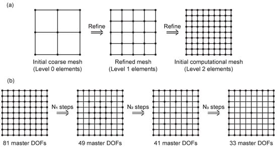
Figure 1.
Illustration of adaptive DOFs condensation: (a) Form the initial computational mesh. (b) Condense the DOFs with the computation time step.
For the transient heat-conduction problem, temperature is the scale variable, and each node corresponds to a temperature DOF, respectively. Then, the process of DOFs condensation with the computation time step is shown in Figure 1. The calculation process of ADOF-FEM is shown in the Figure 2.
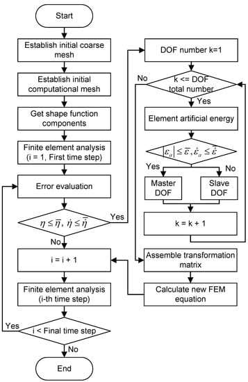
Figure 2.
Flow diagram of ADOF-FEM.
- Establish the initial coarse mesh according to the practical problem of transient heat conduction.
- Considering the requirements of the problem, the user presets the refinement process of the coarse mesh and establishes the initial computational mesh. Then, the program obtains the shape function components between the different levels of the elements.
- Begin the transient temperature-field calculation using the initial computational mesh.
- Calculate the global error of the current time step by error evaluation. When the global error is less than the prespecified tolerance value, judge whether the coarsening criterion is met. Define the DOFs that meet the coarsening criterion as slave DOFs, while the rest are master DOFs.
- Assemble the transformation matrix according to the shape function component and the information of master and slave DOFs.
- Calculate the new FEM basic equation according to the transformation matrix and solve for the unknown variable of master DOFs.
- Solve for the unknown variable of slave DOFs using the transformation matrix according to the solution of the unknown variable of master DOFs.
- Continue to compute the solution of the next time step.
In addition, it is worth noting that when using ADOF-FEM, as the slave DOFs are condensed, the contributions of the slave DOFs to the conductivity matrix need to be accumulated onto the master DOFs according to the transformation matrix, which increase the bandwidth of the matrix. However, since the transformation relationship between master and slave degrees of freedom is local and only a small range of slave degrees of freedom contribute to the corresponding master degrees of freedom, the increase in bandwidth should also be limited and the whole conduction matrix remains a diagonal sparse matrix.
3. Numerical Example
3.1. Example 1
In order to verify that the adaptive DOFs condensation algorithm can effectively reduce the computational cost of the transient temperature field with a small loss of accuracy, the first example is a two-dimensional transient heat-transfer problem without a heat source, whose computational domain is unchanged [40]. In this paper, we calculate the results of different numbers of elements with and without adaptive DOFs condensation and record the computational time. The calculation results are then compared with the analytical solutions to show the changes in computational accuracy.
Suppose that there is an infinitely long steel block with cross-section that is mm, a heat-conduction coefficient of steel k = 25 W/(m · °C), a density of steel , specific heat = 500 J/(kg · °C), and the surface heat-transfer coefficient between the steel and the external medium h = 2000 W/(m · °C). The initial temperature of steel and the temperature of the external medium . The coordinate origin is in the center of the cross-section.
The analytical solutions of temperature in different regions of steel block can be obtained by the separation of variables method (SVM) and Newman’s multiplication theorem. The specific expression of the analytical equation of temperature can be found in the paper.
In this paper, we take the internal position coordinates (0,0), (25,0), (50,0), and (75,0) and the surface position coordinate (100,0) of the steel block as the analysis positions and then use the meshes with different numbers of elements to calculate the FEM results. The initial coarse mesh is divided evenly into square elements, each element is 10 mm long, and the mesh contains a total of 400 elements and 441 nodes. On the basis of the coarse mesh, it is refined 1 and 2 times, and the refined meshes, which are named refined1 and refined2, contain 1600 elements and 6400 elements, respectively. The FEM time step is 1 s, and a total of 3600 steps are calculated.
In order to show the advantages of ADOF-FEM in using the refined model to calculate the transient temperature, we first measured the finite element computational time with and without adaptive DOFs. In this paper, Intel MKL PARDISO is used as the solution method of the FEM equation. The total computational time mainly includes assembling the global conductivity matrix, setting DOFs, matrix factorization, and solving the equation. Table 1 shows the computational time of Example 1 with and without adaptive DOFs for different numbers of elements. As can be seen from Table 1, the main computational cost is matrix factorization, followed by solving the equation and assembling the global conductivity matrix (the more numerous the elements, the higher the computational cost). When ADOF-FEM is used, the interpolation relationship between master and slave DOFs needs to be judged when assembling the global conductivity matrix, and DOFs needs to be set several times in the whole calculation process, so the computational cost of these two parts increases. However, because of the size of the equation, that is, because the number of DOFs can be reduced gradually based on the calculation results, the matrix factorization time can be saved effectively, which accounts for about 80% of the total time. As shown in Figure 3, it shows how the number of DOFs changes over time when ADOF-FEM is used. The computational domain of example 1 is invariant, so the DOFs of Example 1 are gradually condensed when using ADOF-FEM. When the time reaches half of the simulation time, the master DOFs used for calculation are those on the boundary and the lowest level DOFs in the coarse mesh. The process of DOFs change is similar to that demonstrated in Figure 1b, which basically reaches the limit of what can be condensed, so the number of DOFs no longer changes.

Table 1.
The computational time of Example 1 (Unit: ms).
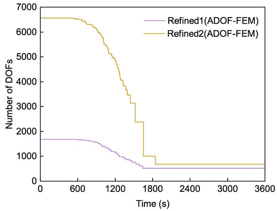
Figure 3.
The change of the number of DOFs in Example 1.
Therefore, the use of ADOF-FEM can reduce the total cost of calculating the transient temperature field, and the more elements, the more cost is saved. The computational time of Refined1 with adaptive DOFs is 82.26% of that without adaptive DOFs, while the computational time of Refined2 with adaptive DOFs is only 61.03% of that without adaptive DOFs. Therefore, the more elements there are, the higher the computational cost, which can be saved by using ADOF-FEM.
In addition to discussing the advantages of ADOF-FEM in saving computational cost, it is also necessary to analyze the accuracy of the algorithm, that is, whether there is a large loss of accuracy leading to the distortion of the calculation results. In this paper, the root mean square error (RMSE) between the FEM result and the analytical solution is used to represent the accuracy in the computational time domain. The RMSE of the FEM result with or without adaptive DOFs is shown in Table 2, where the master DOFs at positions (0,0), (50,0), and (100,0) are unchanged and the master DOFs at positions (25,0), (75,0) are transformed into the slave DOFs when using ADOF-FEM.

Table 2.
The RMSE of the result of Example 1.
As can be seen from Table 2, the calculation accuracy of the finite element increases with the increase of the number of elements, which is consistent with the general law. The RMSE results of refined meshes with adapive DOFs are slightly different from those of the original refined meshes; in other words, when using ADOF-FEM there is only a small loss of the accuracy, and even better accuracy at few positions due to a coincidence of calculation conditions. Combined with Figure 3, it can be seen that the number of DOFs of the refined meshes gradually decreases with time, which is close to the number of DOFs of the coarse mesh eventually, but the accuracy of the refined mesh with adaptive DOFs is much higher than that of the coarse mesh.
In addition, the loss of the accuracy is also different at different positions. The accuracy on the surface can be consistent with that of the refined mesh since the DOFs on the surface are not condensed, while the loss of the accuracy at position (50,0) is greater than that of other positions, which is due to a large number of DOFs near this position condensed at the same time. Moreover, the improvement in accuracy at position (75,0) may be due to the fact that its relative error after the transformation of the master DOF to the slave DOF is independent of the cumulative error in the previous time step caused by the time discretization of that DOF. Figure 4, respectively, shows the relative error between the FEM result and the analytical solution at positions (50,0) and (75,0).
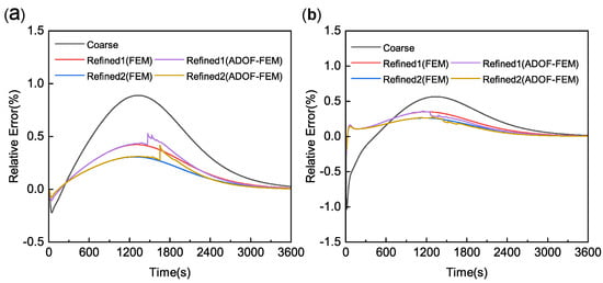
Figure 4.
Relative error at typical positions of Example 1: (a) relative error at position (50,0). (b) Relative error at position (75,0).
By comparing the relative errors of Refined1 and Refined2 with or without adaptive DOFs in Figure 4a, it can be seen that the maximum relative error at position (50,0) of Refined1 with adaptive DOFs is not larger than that of the initial coarse mesh, and the maximum relative error of Refined2 with adaptive DOFs is only slightly larger than that of Refined1, which indicates that the timing of adaptive condensation of DOFs is appropriate. As some of the master DOFs transform into slave DOFs, the other untransformed master DOFs do not introduce large errors.
As can be seen from Figure 4b, due to the small number of elements in the initial coarse mesh, the position (75,0) has no corresponding DOFs, and its result is calculated by the linear interpolation of the DOFs of the elements it is in, which has very poor accuracy, while in Refined1 and Refined2, the corresponding positions have DOFs and the calculation accuracy is much better than that of the initial coarse mesh when the temperature gradient is large initially. When using ADOF-FEM, the position (75,0) is transformed from the master DOF into the slave DOF, and its value is obtained by the linear interpolation of the surrounding master DOFs. At this time, the relative error at the position is only related to that of the surrounding master DOFs and not to the error of this DOF itself due to discretization. According to the previous content, the relative error of the other unchanged master DOFs is small on its own, while the additional error introduced by the DOF transformed based on the coarsening criterion is less than the error tolerance. Therefore, the relative error can be controlled within a small range when the master DOF is transformed into the slave DOF.
Furthermore, although the number of DOFs continues to decrease, the loss of accuracy gradually decreases instead of increasing, which indicates that when the temperature of this position is gradually stable, fewer DOFs can meet the computational accuracy requirements. Based on the above performance, ADOF-FEM effectively takes into account both the computational cost and the computational accuracy requirements.
3.2. Example 2
The objective of this paper is to simulate the temperature field in the construction process of asphalt concrete, so the computational domain of transient heat transfer should be considered to change with time. Example 2 verifies the applicability of ADOF-FEM in the variable computational domain where the variable computational domain is simulated by the birth–death element method. More specifically, the parts have been constructed to participate in the calculation as birth elements, while the parts that have not been constructed are defined as death elements that do not participate in the calculation. With the progress of construction, the death elements are gradually transformed into the birth elements.
Example 2 has four layers of asphalt concrete, and the height and width of each layer are 30 cm and 60 cm, respectively. The parameters of the material are as follows: the heat-conduction coefficient of asphalt concrete , the density of asphalt concrete , the specific heat , and the surface heat-transfer coefficient between the asphalt concrete and the air outside . The initial temperature of each layer of asphalt concrete , and the temperature of the air outside is . The boundary conditions of the model are as follows: the upper surface and the two sides are the heat dissipation boundary (the third type of boundary conditions), and the bottom surface is the adiabatic boundary. The calculation condition is that each layer dissipates heat for 12 h, and then the latter layer is started to construct, that is, the construction interval is 12 h.
The FEM mesh of Example 2 is shown in the Figure 5. The initial coarse mesh contains a total of 288 elements and 325 nodes, and the initial computational mesh which contains 4608 elements and 4753 nodes, is refined two times on the basis of the coarse mesh. The computational time domain includes the heat dissipation for 12 h after the construction of the first three layers and the overall heat dissipation for 120 h after all the construction where the FEM time step is fixed as 1 min. In fact, the construction of the latter layer will have a great influence on the temperature of the previous layer. In order to avoid the large error, Example 2 is required to condense the DOFs of the previous layer (except for the last layer) only after the construction of the latter layer is completed.
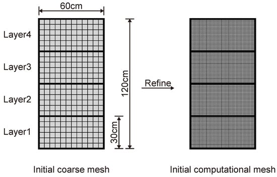
Figure 5.
The FEM mesh of Example 2.
Figure 6 shows the FEM results of the temperature field based on the initial computational mesh, and Figure 7 shows the FEM results with adaptive DOFs. Figure 8 shows the distribution of master and slave DOFs of the model when ADOF-FEM is used. It can be seen that the temperature field in the construction process of asphalt concrete is actually the heat transfer from the new layer to the old layers. The points with a large temperature gradient are basically distributed in the new layer and then move down slowly with time. At the same time, the value of the temperature gradient also gradually decreases with time, and this is also reflected in the change of the condensation range of DOFs. The results calculated by using ADOF-FEM are a little rougher than those calculated by using all of the DOFs, but their distribution is consistent and the error is relatively small. Therefore, when the transient temperature field of the asphalt-concrete core wall construction is simulated by FEM, using ADOF-FEM can still obtain satisfactory results.
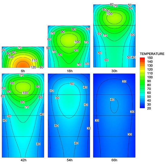
Figure 6.
The temperature contour of Example 2 (FEM).
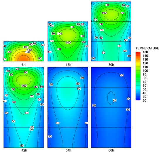
Figure 7.
The temperature contour of Example 2 (ADOF-FEM).
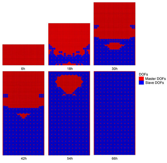
Figure 8.
The distribution of DOFs of Example 2 (ADOF-FEM).
Figure 9 compares the changes of the DOFs of the model over time steps with or without using ADOF-FEM and shows their total computational time. The computational domain of Example 2 is variable, so each time the computational domain is increased some new DOFs are added, while the DOFs condensation proceeds in parallel. So, the number of DOFs is first increased, then slowly reduced, and then increased again. When the computational domain is no longer increasing, the number of DOFs in Example 2 changes similarly to Example 1, and eventually, the number of DOFs no longer changes. It can be seen that in the FEM simulation of the transient temperature field of the asphalt concrete construction, the number of DOFs gradually increases as the computational domain gradually increases, but after using ADOF-FEM, the number of DOFs can be controlled within a range. A period of time after the end of construction, more DOFs can be condensed as the temperature gradient gradually becomes smooth because at this time a smaller number of DOFs can be used to obtain a good result. In Example 2, the final number of DOFs when using ADOF-FEM is only 10% of that used in FEM, and about 60% of the computational time can be saved.
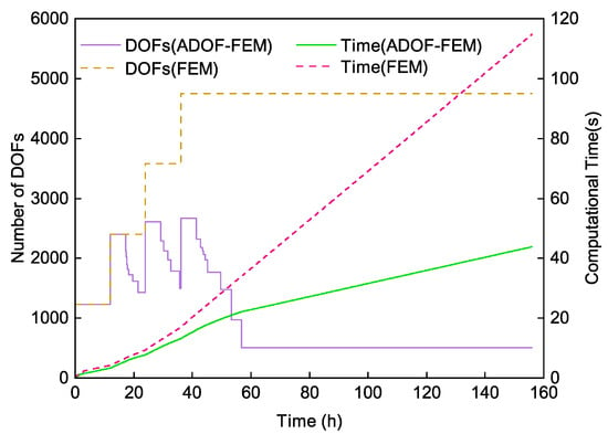
Figure 9.
The change of the number of DOFs and computational time in Example 2.
In conclusion, for the long-term transient heat-transfer problem of asphalt concrete during construction considering the variable computational domain, ADOF-FEM can calculate satisfactory temperature results with little computational cost.
3.3. Example 3
The Yinchaojiliao Project is currently the largest water-conservancy project in Inner Mongolia, China. As an important part of the project, the Wendegen water control project is an ultra-long asphalt-concrete core dam under construction in the cold region. The maximum dam height is 48 m, and the total length of the dam is 1358 m. Due to the large scale of the project and the limited time available for construction, the dam was constructed in sections. However, large day and night temperature differences or long overwintering low-temperature conditions can easily lead to unhealable cracks between the core wall sections or the construction layers. In order to guarantee the quality of the asphalt-concrete core wall from the temperature control point of view, it is necessary to firstly simulate the temperature field for the whole construction process of the asphalt-concrete core wall and then use this as a basis for calculating the temperature stress in each part.
The project was designed and built a large scale on-site solid model to facilitate the study of the laws governing the construction quality of core wall. The model was selected from an actual 80 m long dam with the height of the dam as the scaled dimension, and the scale of the model was 1:10. As shown in Figure 10 and Figure 11, the length of the model is 19.6 m, the width is 16.8 m, and the height is 4.8 m. The slope ratio of upstream and downstream is 1:1.5, and that on the left and right banks is 1:1. The core wall in the model has a length of 8.0 m, a width of 0.6 m, and a height of 4.8 m. The core wall and rockfill material are constructed with 0.3 m as a layer, with a total of 16 layers. The FEM model, which is shown in Figure 12, is established based on the on-site solid model. The FEM model includes the initial coarse mesh and the refined computational mesh based on the coarse mesh. The coarse mesh provides the basic information of the FEM model, but it does not have the ability to simulate the whole process dynamically. Compared with the coarse mesh, the refined mesh can simulate the construction process and has higher accuracy, but its computational cost is large. It is assumed that the initial temperatures of each layer of asphalt concrete and rockfill material are and , respectively, and the temperature of the air outside is . The thermal parameters of asphalt concrete are the same as in Example 2. The parameters of the rockfill material are as follows: the heat-conduction coefficient of the rockfill material , the density of the rockfill material , the specific heat , and the surface heat-transfer coefficient between the asphalt concrete and the air outside . The boundary conditions of Example 3 are as follows: the bottom surface is the adiabatic boundary, and the other outer surfaces are the heat dissipation boundary. The calculation condition is that each layer dissipates heat for 12 h and then the construction of the latter layer begins, that is, the construction interval is 12 h.
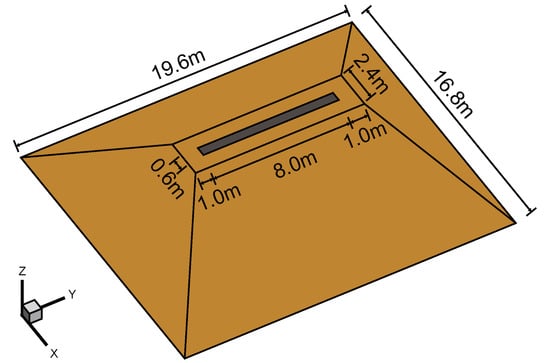
Figure 10.
The size of Example 3 model.
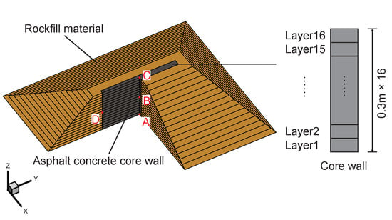
Figure 11.
The component of Example 3 model.
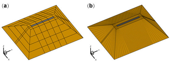
Figure 12.
The mesh of Example 3: (a) The initial coarse mesh. (b) The initial computational mesh.
The total time step of Example 3 is 420 h. Figure 13 shows the temperature contour in vertical and cross sections of Example 3 at four typical times when using ADOF-FEM. From Figure 13, they are, respectively, 12 h after the completion of the 4th layer, 12 h after the completion of the 8th layer, 12 h after the completion of all construction, and 120 h after the completion of all construction, which in total are, respectively, 48 h, 96 h, 192 h, and 300 h. It can be seen that the results calculated with adaptive DOFs are smooth without abnormal areas or values, and the results are consistent with the distribution law of the temperature field of asphalt-concrete core wall construction. Since the FEM calculation results are basically the same as the ADOF-FEM calculation results, only the ADOF-FEM results are included in Figure 13 as a demonstration. At the same time, four typical point positions, which are shown in Figure 11, are selected to compare the results with and without adaptive DOFs. Points A, B, and C are located in the center of the core wall, respectively, at the bottom of the 1st layer, the middle of the 8th layer, and the top of the 16th layer. Point D is located at the contact position between the core wall and the rockfill material at the same elevation as Point B. The comparison results are shown in Figure 14, and it can be seen that the difference of results with and without adaptive DOFs is small, which indicates that it is feasible to use ADOF-FEM to solve the simulation problem of the transient temperature field during the construction period of the asphalt-concrete core wall.
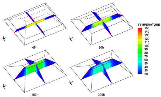
Figure 13.
The temperature contour in vertical and cross sections of Example 3.
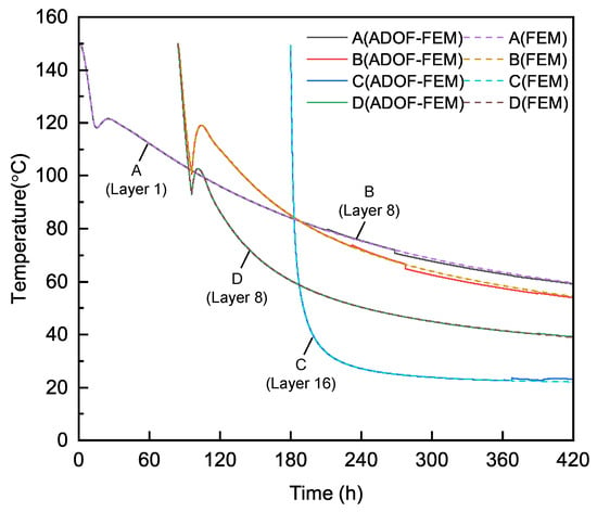
Figure 14.
The temperature at typical point positions of Example 3.
The computational time and the number of DOFs for Example 3 are shown in Figure 15, which vary similarly to Example 2. By using ADOF-FEM, the DOFs of Example 3 can be saved up to 70% and the computational time can be saved by approximately 40%. When using ADOF-FEM to condense the DOFs, all of the elements and DOFs in the model exist objectively and are assembled into the global conductivity matrix in a cyclic traversal. ADOF-FEM only changes the assembly process of DOFs based on the transformation matrix, so the time to assemble the global conductivity matrix cannot be saved, and the only time saved by ADOF-FEM is the matrix factorization and equation solution. Even so, ADOF-FEM is helpful when using a large 3D finite element model to simulate the temperature field for the whole construction process of the asphalt-concrete core wall.
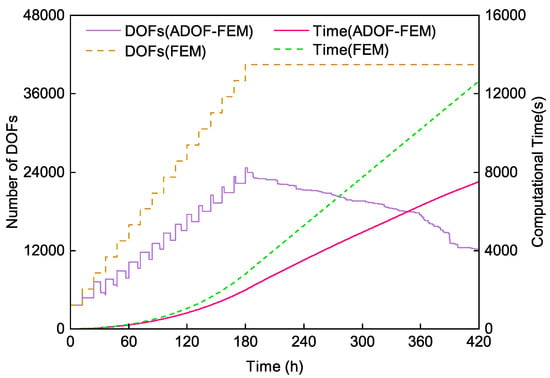
Figure 15.
The change of the number of DOFs and computational time in Example 3.
Example 3 is used to simulate the temperature change during the construction of a 16-layer core-wall dam under the same conditions and processes and to verify the applicability of the ADOF-FEM. Since the relevant conditions and processes are generally constant throughout the construction of the core-wall dam, the results of the calculations will have similar characteristics if we continue to extend the construction of the 17th, 18th, and other layers of the core wall. ADOF-FEM can be uesd naturally in a similar way and eventually solve the problem of the high cost of temperature simulation during the construction of the entire asphalt-concrete core-wall dam.
4. Discussion
From the three examples, it can be seen that ADOF-FEM can achieve good results when the computational domain does or does not change with time. This is because when there is no internal heat source and the temperature of the external environment is constant, the temperature in the computational domain gradually approaches a stable value or interval over time, and the spatial distribution of temperature will gradually become gentle over time. At this point, refined mesh and more DOFs are naturally not needed to describe the drastic changes of temperature in time and space, which is the basis for the good performance of ADOF-FEM. At the same time, the transient temperature simulation during the construction of the asphalt-concrete core wall satisfies this situation approximately. Firstly, although asphalt concrete has the initial temperature of construction, there is no internal heat source. Secondly, the core wall is subjected to the thermal insulation effect of rockfill, and the surface of the core wall is affected by the external air temperature being low, due to the fact that the external environment is relatively stable. Therefore, ADOF-FEM can be used to simulate the temperature variation of the asphalt-concrete core wall during the construction period layer by layer with a coordinated mesh.
When simulating the temperature variation of the concrete construction process or that of material adding layer by layer in additive manufacturing, the so-called zone-merged algorithm is often used. In essence, this algorithm is controlled by the user to merge multiple construction layers into one layer in a calculation step. If this kind of method is applied to the construction process of the asphalt-concrete core, it is complicated to use this method because there may be different positions in the same layer that do or do not need to be merged, and users need to preset the merging time and the merging scope. The ADOF-FEM can adaptively condense the DOFs for different positions based on the prespecified tolerance value of the judgment criterion, and it can set multiple levels of DOFs according to the number of times the mesh is refined. The different levels of DOFs can be condensed according to the judgment criteria under the same frame, so this method is simpler. It is worth noting that the prespecified tolerance value of coarsening judgment criteria is defined by users. For the asphalt-concrete core-wall dam, it has a fixed construction technology, and the temperature distribution of the different core-wall layers has common characteristics. Therefore, the temperature variation of several layers of the core-wall construction process can be pre-analyzed to obtain the appropriate prespecified tolerance value, and then the temperature of the whole core-wall dam during the construction period can be analyzed.
It can be seen from the three examples that the error of the calculation results caused by ADOF-FEM at the position of master DOFs and slave DOFs is small. Compared with the temperature contour in Figure 6 and Figure 7, using ADOF-FEM will make the smooth contour rougher in some positions, but considering that the temperature in these positions is relatively stable in time and space, such a loss of precision is acceptable.
Furthermore, the computational cost saved by ADOF-FEM is mainly the two parts of matrix factorization and solving the equation in FEM because the time spent in these two parts is directly related to the number of DOFs. However, the total computational time also includes assembling the global conductivity matrix, which is related to the number of elements, and ADOF-FEM itself cannot reduce the number of elements in the computational mesh, so it cannot save this part of computational time. Therefore, there is an upper limit in using ADOF-FEM to save the computational cost.
Considering that using the adaptive mesh can reduce the number of elements, if the two methods are combined, the region with more DOFs condensation can reconstruct the mesh adaptively on the appropriate calculation step. By combining many times of adaptive DOFs condensation with few times of adaptive mesh changes and coordinating the timing of the use of the two methods, the huge extra computational cost caused by the repeated changes of the traditional adaptive mesh can be avoided and it may achieve better results.
5. Conclusions
In this paper, we propose the ADOF-FEM algorithm and the corresponding coarsening judgment criterion to solve the problem of the huge computational cost of the asphalt-concrete core-wall transient temperature simulation during the construction period. Additionally, the computational cost is reduced by adaptively condense DOFs. We use two numerical examples, respectively, to verify that ADOF-FEM can effectively reduce the cost of matrix factorization and solve the equation in FEM at the cost of minor precision loss in the long-term transient temperature simulation whose computational domain is or is not unchanged. Then, an example with an engineering background is used to verify that ADOF-FEM can reduce approximately 70% of DOFs and save more than 40% of the computational cost when simulating the transient temperature of the asphalt-concrete core wall during the construction period.
Author Contributions
Conceptualization, L.Y. and T.L.; methodology, L.Y.; software, L.Y.; validation, L.Y. and H.Q.; formal analysis, L.Y.; investigation, L.Y., H.L., and F.W.; resources, T.L. and H.L.; data curation, L.Y.; writing—original draft preparation, L.Y.; writing—review and editing, L.Y.; visualization, L.Y.; supervision, T.L.; project administration, T.L.; and funding acquisition, T.L. All authors have read and agreed to the published version of the manuscript.
Funding
This research was financially supported by the National Key Research and Development Plan (SN: 2022YFC3005403), the Science and Technology Project of Inner Mongolia Yinchaojiliao Project (SN:YC-KYXM-04-2020), the Science and Technology Project of Water Resources Department of Jiangxi Province (SN:202224ZDKT14), and the National Natural Science Foundation of China (SN: 52009035).
Institutional Review Board Statement
Not applicable.
Informed Consent Statement
Not applicable.
Data Availability Statement
Not applicable.
Conflicts of Interest
The authors declare no conflict of interest. The funders had no role in the design of the study; in the collection, analyses, or interpretation of data; in the writing of the manuscript; or in the decision to publish the results.
Abbreviations
The following abbreviations are used in this manuscript:
| DOF | Degree of freedom |
| FEM | Finite element method |
| ADOF-FEM | Adaptive degree of freedom—finite element method |
| SVM | Separation of variables method |
| RMSE | Root mean square error |
References
- ICOLD. Asphalt-Concrete Cores for Embankment Dams; Bulletin 179; International Commission on Large Dams: Paris, France, 2018. [Google Scholar]
- Höeg, K. Asphaltic Concrete Cores for Embankment Dams; Norwegian Geotechnical Institute: Oslo, Norway, 1993. [Google Scholar]
- Pircher, W.; Schwab, H. Design, construction, and behavior of the asphaltic concrete core wall of the Finstertal Dam. In Proceedings of the 16th Congress of the International Commission on Large Dams, San Francisco, CA, USA, 13–17 June 1988; Calif. ICOLD Press: Paris, France, 1988; Volume 2, pp. 901–924. [Google Scholar]
- Wang, W.; Höeg, K.; Zhang, Y. Design and performance of the Yele asphalt-core rockfill dam. Can. Geotech. J. 2010, 47, 1365–1381. [Google Scholar] [CrossRef]
- Feng, S.; Wang, W.; Hu, W.; Deng, Y.; Yang, J.; Wu, S.; Zhang, C.; Höeg, K. Design and performance of the Quxue asphalt-core rockfill dam. Soils Found. 2020, 60, 1036–1049. [Google Scholar] [CrossRef]
- Chen, S.; Gu, C.; Lin, C.; Zhang, K.; Zhu, Y. Multi-kernel optimized relevance vector machine for probabilistic prediction of concrete dam displacement. Eng. Comput. 2020, 37, 1943–1959. [Google Scholar] [CrossRef]
- Lin, C.; Li, T.; Chen, S.; Yuan, L.; van Gelder, P.; Yorke-Smith, N. Long-term viscoelastic deformation monitoring of a concrete dam: A multi-output surrogate model approach for parameter identification. Eng. Struct. 2022, 266, 114553. [Google Scholar] [CrossRef]
- Kim, Y.R. Modeling of Asphalt Concrete; McGraw-Hill Education: New York, NY, USA, 2009. [Google Scholar]
- Ning, Z.; Liu, Y.; Wang, W. Compressive Behavior of Hydraulic Asphalt Concrete under Different Temperatures and Strain Rates. J. Mater. Civ. Eng. 2021, 33, 04021013. [Google Scholar] [CrossRef]
- Smesnik, M.; Krstic, S.; Guven, S.; Verdianz, M. Asphalt core embankment dams in turkey–dam design, core material and construction. In Proceedings of the ICOLD—European Club Symposium, Crete, Greece, 2–4 October 2019; pp. 1–10. [Google Scholar]
- Ding, J.; Colegrove, P.; Mehnen, J.; Ganguly, S.; Almeida, P.S.; Wang, F.; Williams, S. Thermo-mechanical analysis of Wire and Arc Additive Layer Manufacturing process on large multi-layer parts. Comput. Mater. Sci. 2011, 50, 3315–3322. [Google Scholar] [CrossRef]
- Compton, B.G.; Post, B.K.; Duty, C.E.; Love, L.; Kunc, V. Thermal analysis of additive manufacturing of large-scale thermoplastic polymer composites. Addit. Manuf. 2017, 17, 77–86. [Google Scholar] [CrossRef]
- Liu, Y.; Zhang, J.; Pang, Z. Numerical and experimental investigation into the subsequent thermal cycling during selective laser melting of multi-layer 316L stainless steel. Opt. Laser Technol. 2018, 98, 23–32. [Google Scholar] [CrossRef]
- Fetni, S.; Enrici, T.M.; Niccolini, T.; Tran, H.S.; Dedry, O.; Duchêne, L.; Mertens, A.; Habraken, A.M. Thermal model for the directed energy deposition of composite coatings of 316L stainless steel enriched with tungsten carbides. Mater. Des. 2021, 204, 109661. [Google Scholar] [CrossRef]
- Denlinger, E.R.; Irwin, J.; Michaleris, P. Thermomechanical modeling of additive manufacturing large parts. J. Manuf. Sci. Eng. 2014, 136, 061007. [Google Scholar] [CrossRef]
- Hajializadeh, F.; Ince, A. Finite element–based numerical modeling framework for additive manufacturing process. Mater. Des. Process. Commun. 2019, 1, e28. [Google Scholar] [CrossRef]
- Montevecchi, F.; Venturini, G.; Grossi, N.; Scippa, A.; Campatelli, G. Finite Element mesh coarsening for effective distortion prediction in Wire Arc Additive Manufacturing. Addit. Manuf. 2017, 18, 145–155. [Google Scholar] [CrossRef]
- Ren, K.; Chew, Y.; Zhang, Y.; Bi, G.; Fuh, J. Thermal analyses for optimal scanning pattern evaluation in laser aided additive manufacturing. J. Mater. Process. Technol. 2019, 271, 178–188. [Google Scholar] [CrossRef]
- Staten, M.L.; Benzley, S.; Scott, M. A methodology for quadrilateral finite element mesh coarsening. Eng. Comput. 2008, 24, 241–251. [Google Scholar] [CrossRef]
- Shepherd, J.F.; Dewey, M.W.; Woodbury, A.C.; Benzley, S.E.; Staten, M.L.; Owen, S.J. Adaptive mesh coarsening for quadrilateral and hexahedral meshes. Finite Elem. Anal. Des. 2010, 46, 17–32. [Google Scholar] [CrossRef]
- Kirk, B.S.; Peterson, J.W.; Stogner, R.H.; Carey, G.F. libMesh: A C++ library for parallel adaptive mesh refinement/coarsening simulations. Eng. Comput. 2006, 22, 237–254. [Google Scholar] [CrossRef]
- Baiges, J.; Bayona, C. Refficientlib: An Efficient Load-Rebalanced Adaptive Mesh Refinement Algorithm for High-Performance Computational Physics Meshes. SIAM J. Sci. Comput. 2017, 39, C65–C95. [Google Scholar] [CrossRef]
- Moreira, C.A.; Caicedo, M.A.; Cervera, M.; Chiumenti, M.; Baiges, J. A multi-criteria h-adaptive finite-element framework for industrial part-scale thermal analysis in additive manufacturing processes. Eng. Comput. 2022, 38, 4791–4813. [Google Scholar] [CrossRef]
- Li, C.; Denlinger, E.R.; Gouge, M.F.; Irwin, J.E.; Michaleris, P. Numerical verification of an Octree mesh coarsening strategy for simulating additive manufacturing processes. Addit. Manuf. 2019, 30, 100903. [Google Scholar] [CrossRef]
- Qu, Z.Q. Model Order Reduction Techniques; Springer: London, UK, 2004. [Google Scholar] [CrossRef]
- Guyan, R.J. Reduction of stiffness and mass matrices. AIAA J. 1965, 3, 380. [Google Scholar] [CrossRef]
- Henshell, R.D.; Ong, J.H. Automatic masters for eigenvalue economization. Earthq. Eng. Struct. Dyn. 1974, 3, 375–383. [Google Scholar] [CrossRef]
- Leung, A.Y.T. An accurate method of dynamic condensation in structural analysis. Int. J. Numer. Methods Eng. 1978, 12, 1705–1715. [Google Scholar] [CrossRef]
- Archer, G.C. A technique for the reduction of dynamic degrees of freedom. Earthq. Eng. Struct. Dyn. 2000, 30, 127–145. [Google Scholar] [CrossRef]
- ANSYS, Inc. ANSYS Mechanical APDL Theory Reference; ANSYS, Inc.: San Jose, CA, USA, 2020. [Google Scholar]
- Llau, A.; Jason, L.; Dufour, F.; Baroth, J. Adaptive zooming method for the analysis of large structures with localized nonlinearities. Finite Elem. Anal. Des. 2015, 106, 73–84. [Google Scholar] [CrossRef]
- Mezher, A.; Jason, L.; Folzan, G.; Davenne, L. Simulation of large dimensional reinforced and prestressed concrete structures using a new adaptive static condensation method including automatic mesh partitioning. Finite Elem. Anal. Des. 2022, 202, 103718. [Google Scholar] [CrossRef]
- Zhang, Y.; Ho, S.L.; Fu, W.; Wu, H. An adaptive degrees-of-freedom finite element method for 3-D nonlinear magneto-thermal field analysis. Numer. Heat Transf. Part A Appl. 2019, 75, 523–532. [Google Scholar] [CrossRef]
- Lewis, R.W.; Nithiarasu, P.; Seetharamu, K.N. Fundamentals of the Finite Element Method for Heat and Fluid Flow; John Wiley & Sons: Hoboken, NJ, USA, 2004. [Google Scholar]
- Katona, M.C.; Zienkiewicz, O.C. A unified set of single step algorithms part 3: The beta-m method, a generalization of the Newmark scheme. Int. J. Numer. Methods Eng. 1985, 21, 1345–1359. [Google Scholar] [CrossRef]
- Zienkiewicz, O.C.; Zhu, J.Z. A simple error estimator and adaptive procedure for practical engineerng analysis. Int. J. Numer. Methods Eng. 1987, 24, 337–357. [Google Scholar] [CrossRef]
- Franca, A.S.; Haghighi, K. Adaptive Finite Element Analysis of Transient Thermal Problems. Numer. Heat Transf. Part B Fundam. 1994, 26, 273–292. [Google Scholar] [CrossRef]
- Lewis, R.W.; Huang, H.C.; Usmani, A.S.; Cross, J.T. Finite element analysis of heat transfer and flow problems using adaptive remeshing including application to solidification problems. Int. J. Numer. Methods Eng. 1991, 32, 767–781. [Google Scholar] [CrossRef]
- Denlinger, E.R. Development and Numerical Verification of a Dynamic Adaptive Mesh Coarsening Strategy for Simulating Laser Power Bed Fusion Processes. In Thermo-Mechanical Modeling of Additive Manufacturing; Elsevier: Amsterdam, The Netherlands, 2018; pp. 199–213. [Google Scholar] [CrossRef]
- Huiping, L.; Guoqun, Z.; Shanting, N.; Chuanzhen, H. FEM simulation of quenching process and experimental verification of simulation results. Mater. Sci. Eng. A 2007, 452–453, 705–714. [Google Scholar] [CrossRef]
Disclaimer/Publisher’s Note: The statements, opinions and data contained in all publications are solely those of the individual author(s) and contributor(s) and not of MDPI and/or the editor(s). MDPI and/or the editor(s) disclaim responsibility for any injury to people or property resulting from any ideas, methods, instructions or products referred to in the content. |
© 2023 by the authors. Licensee MDPI, Basel, Switzerland. This article is an open access article distributed under the terms and conditions of the Creative Commons Attribution (CC BY) license (https://creativecommons.org/licenses/by/4.0/).