Resonance Detection Method and Realization of Bearing Fault Signal Based on Kalman Filter and Spectrum Analysis

Abstract

The rolling bearing is an important part of mechanical equipment, and its performance significantly affects the quality and life of the mechanical equipment. This article uses the integrated fiber Bragg grating resonant structure sensor excited by periodic micro-shocks caused by micro faults to realize the extraction of information relating to potential faults. Because the fault signal is weak and can easily be interfered with by ambient noise, in order to extract the effective signal, this article determines the autoregressive model of bearing vibration by the final prediction error criterion and the recursive least squares estimation algorithm. The augmented state space model is established based on the autoregressive model. A Kalman filter is used to reduce the noise interference, and then the reduction noisy signal is analyzed by power spectrum and improved autocorrelation envelope spectrum to realize the detection of bearing faults. Through data analysis and method comparison, the proposed improved autocorrelation envelope spectrum analysis can directly extract the bearing fault frequency, which is superior to other methods such as cepstral analysis.

1. Introduction

A bearing is a basic and important component in rotating machinery. Generally, there are many kinds of noises in the working environment. The load during operation is also relatively large and easily damaged. Early bearing failures can be hidden in machine vibration and environmental noise [1]. In serious cases, bearing failure will affect the normal operation of the whole equipment and pose a threat to the operation of the equipment. Therefore, the detection and fault diagnosis of the bearing are of great significance [2,3].

The incipient shock of the rolling bearing is weak, the contact interface damage is small, the shock force generated by the interaction of the components is not large, and the vibration amplitudes and the characteristic information are not obvious and weak. Due to the constraints of the space structure, the bearing is usually not directly measured, and data can only be obtained indirectly through the sensor installed on the equipment bearing seat or in an external housing. The fault impulse response will be attenuated in the mediating parts between the bearing and the sensor. In addition, it is difficult to avoid the interference of component vibration and sensor circuit conversion noise during the operation of the equipment. Therefore, the signal-to-noise ratio of the final picked-up signal is usually low, and the proportion of the relevant component of the fault in the signal is small [4,5]. In addition, the rolling elements may slide relative to each other or sway due to uneven force. Therefore, the interval between fault shocks is not strictly consistent. Additionally, when the bearing speed is too high, some rolling elements will fly by before the collision fault point, resulting in the loss of fault shock. Many of the above factors have presented great obstacles to the identification of faults of bearings. Therefore, seeking an effective and reliable method for extracting weak fault features has always been a prominent and difficult point in engineering application research. At the same time, it has important practical significance for the monitoring and forecasting of the equipment’s status and for later equipment maintenance [6,7].

At present, the research on fault detection and diagnosis of rolling bearings has made certain progress. Djebala et al. directly used discrete wavelet transform to identify early bearing faults, and successfully extracted weak feature information after signal decomposition and reconstruction, but the wavelet transform needs to select a suitable wavelet threshold and a suitable number of wavelet decomposition layers [8]. Wang et al. studied the method of extracting the weak feature of the bearing, which combined the adjustable quality factor wavelet transform and the aggregate empirical mode decomposition, and successfully applied it to the actual signal analysis, but the empirical mode decomposition has problems of mode aliasing and end effects, and it is necessary to select a sufficient number of eigenmode functions [9]. Jiang et al. used the minimum direct deconvolution to filter the early fault signals of the bearing, and used the full-period signal of the bearing to verify that the characteristics of the fault signal after noise reduction can be more obvious, but the minimum direct deconvolution is a non-globally-optimal filter, which has poor robustness and is susceptible to interference from a few abnormal spikes during signal processing [10]. Yao et al. used enhanced sparse representation algorithm based on an adaptive period matching to extract the initial fault features of the bearing [11]. Wang et al. combined the signal processing with ensemble bagged-trees-based machine learning and used the decomposition and reconstruction methods in the stochastic resonance to diagnose early bearing fault, but the time efficiency of mechanical fault detection of this method needs to be improved [12]. As an intelligent fault diagnosis method, machine learning has been applied to rotating systems fault diagnosis [13]. Rezazadeh et al. proposed a method to identify shallow cracks in rotor systems by using convolutional neural networks and persistent spectra during steady state operation [14]. Then, based on supervised learning and convolutional neural network methods, intelligent methods for automatic detection of imbalance, crack and parallel dislocation in rotating machinery are compared [15]. Using machine learning requires a substantial amount of time and computing power.

In recent years, some researchers have used models to analyze bearing faults. Sawalhi et al. combined AR inverse filtration and squared envelope to estimate the spall size within the bearing [16]. Bastami et al. established an autoregressive model based on discrete wavelet transform to estimate the defects of tapered roller bearings [17]. Wu et al., addressing the stator/rotor winding fault, established the model, analyzed the characteristics, and proposed a new type of robust diagnosis design for stator/rotor winding early fault [18]. Borghesani et al. studied the signal model of rolling bearings and evaluated the stationarity of real and pseudo cycles in the rolling bearing signal, as well as the first and second order (pseudo) cycle stationary fault symptoms [19].

The autoregressive models based on time series analysis have a wide range of applications in signal processing, and have certain applications in bearing fault detection and bearing life-prediction. It establishes a statistical model based on a finite-length sample, and then uses the model to achieve prediction, filtering or control purposes. The model parameters contain important state characteristics of the system and are very sensitive to system state changes. The autoregressive model can also be transformed with the state space model, in which it is convenient to use Kalman filter for noise reduction. The Kalman filter is a time domain method. The recursive algorithm is used, which is convenient for real-time implementation on the computer, with small computation and storage, and it can handle multi-variable, time-varying, and non-stationary time series filtering problems. With the Kalman filter, the system state is specified and defined in combination with specific problems, which can reflect the characteristics and conditions of the system, which is conducive to solving practical problems [20].

Considering the limitations of the methods in the literature cited above, combined with the advantages of the autoregressive model and the Kalman filter, this article is based on the analysis of bearing vibration signals detected by fiber Bragg grating resonant sensors. First, it establishes a state space model of rolling bearing based on the autoregressive model of time series. The recursive least squares estimation algorithm is used to determine the model parameters, the final error prediction criterion is used to determine the model order, and the autocorrelation function is used to verify the tailing of the autoregressive model. Then, the Kalman filter is applied to the vibration signal to realize signal noise reduction processing. The noise-reduced signal is first analyzed by power spectrum to detect whether the bearing has fault. If a fault occurs, improved autocorrelation envelope spectrum analysis is used to determine the location of the bearing fault. Finally, it is compared with the analysis result of wavelet transform and empirical mode decomposition to verify the accuracy and effectiveness of the method in this article. The combination of Kalman filter and spectrum analysis can effectively extract the evidence of the faulty bearing and realize the fault detection and identification of the rolling bearing.

The main contributions of this article are as follows:

(1)

Based on the vibration signal detected by the fiber Bragg grating resonant sensor, an autoregressive model is established and transformed into a state space model of bearing vibration.

(2)

Based on the established state equation and observation equation of bearing vibration, a Kalman filter is used to realize state estimation and noise reduction.

(3)

Bearing fault diagnosis is realized by the improved autocorrelation envelope spectrum analysis method. The first method proposed is the improved autocorrelation envelope power spectrum, which can extract the fault frequencies and their multipliers. The second method proposed is the autocorrelation envelope maximum entropy spectrum, which can directly extract the bearing failure frequency. The two envelope spectrum lines are pure and the noise interference is small. The bearing fault detection and fault identification are realized.

2. Methods and Principle

2.1. Random Signal Autoregressive Model

An autoregressive model (abbreviated AR model) is analyzed by time series. The information within the system state can be reflected by identifying model parameters. The accurate ordering of descriptors in the AR model can express the system state intensively and accurately in the objective laws of a dynamic system. In addition, studies have shown that the autoregressive parameters of the AR model are very sensitive to the state change law.

The AR model is a linear model. The model uses a difference equation to describe the random sequence. The relationship between the sequence points of different signals is different, so different models are obtained.

$\mathrm{AR}\left(\mathrm{n}\right)$ model is

$$\mathrm{x}\left(\mathrm{k}\right)={\mathsf{\phi }}_1\mathrm{x}\left(\mathrm{k}-1\right)+{\mathsf{\phi }}_2\mathrm{x}\left(\mathrm{k}-2\right)+\cdots +{\mathsf{\phi }}_{\mathrm{n}}\mathrm{x}\left(\mathrm{k}-\mathrm{n}\right)+\mathrm{a}\left(\mathrm{k}\right), \mathrm{a}\left(\mathrm{k}\right)~\mathrm{NID}\left(0,{\mathsf{\sigma }}_{\mathrm{a}}^2\right)$$

(1)

In formula (1), $\mathrm{x}\left(\mathrm{k}\right)$ is observation, k is time series, $\mathrm{k}=1,2,\cdots ,\mathrm{N},$ $\mathrm{a}\left(\mathrm{k}\right)$ is zero-mean Gaussian white noise, $\mathrm{n}$ is the model order. The $\mathrm{AR}$ model describes the relationship between the value of the $\mathrm{k}$-th point in the random sequence $\left\{\mathrm{x}\left(\mathrm{k}\right)\right\}$ and the previous adjacent $\mathrm{n}$ points, and uses a zero-mean Gaussian distribution error term $\mathrm{a}\left(\mathrm{k}\right)$ to represent the uncertainty of the relationship.

2.2. AR Model Order Determination and Parameter Estimation

The smaller the variance of the error term, the more accurate the model, and the more it can simulate the relationship between the items in the sequence.

According to formula (1), it follows that

$$\mathrm{a}\left(\mathrm{k}\right)=\mathrm{x}\left(\mathrm{k}\right)-{\mathsf{\phi }}_1\mathrm{x}\left(\mathrm{k}-1\right)-{\mathsf{\phi }}_2\mathrm{x}\left(\mathrm{k}-2\right)-\cdots -{\mathsf{\phi }}_{\mathrm{n}}\mathrm{x}\left(\mathrm{k}-\mathrm{n}\right)$$

(2)

$${\mathsf{\sigma }}_{\mathrm{a}}^2=\frac{1}{\mathrm{N}-\mathrm{n}}{\displaystyle \sum }_{\mathrm{k}=\mathrm{n}+1}^{\mathrm{N}}{\left(\mathrm{x}\left(\mathrm{k}\right)-{\displaystyle \sum }_{\mathrm{i}=1}^{\mathrm{n}}{\mathsf{\phi }}_{\mathrm{i}}\mathrm{x}\left(\mathrm{k}-\mathrm{i}\right)\right)}^2$$

(3)

In formulas (2) and (3), ${\mathsf{\phi }}_{\mathrm{i}}\left(\mathrm{i}=1,2,\cdots ,\mathrm{n}\right)$ is the parameter of the model. ${\mathsf{\sigma }}_{\mathrm{a}}^2$ is the variance.

When the order n of the AR model is unknown, it needs to be determined in the recursive process. With the increase of model order, the variance of the model decreases gradually. When it reaches the minimum value or no longer changes, the order at this time is the correct order of the AR model.

The model order is determined using final prediction error (FPE) criterion. The FPE criterion is the sum of the power of the unpredictable part of the AR(n) process and the error power caused by inaccurate AR parameter estimation.

The definition formula is as follows:

$$\mathrm{FPE}\left(\mathrm{n}\right)=\frac{\mathrm{N}+\mathrm{n}+1}{\mathrm{N}-\mathrm{n}+1}{\mathsf{\sigma }}_{\mathrm{a}}^2, \mathrm{n}=0,1,\cdots ,\mathrm{L}$$

(4)

In formula (4), L is the highest order given in advance. N is the number of data samples, and the value in parentheses increases as n increases (towards N). It reflects that the inaccuracy of the estimation of the prediction error power is increasing. The minimum value will appear in the process that ${\mathsf{\sigma }}_{\mathrm{a}}^2$ decreases as the order increases. The order corresponding to the minimum value of FPE is the final order. When M is the minimum order, formula (5) is satisfied.

$$\mathrm{FPE}\left(\mathrm{M}\right)=\underset{0\le \mathrm{n}\le \mathrm{L}}{\min }\mathrm{FPE}\left(\mathrm{n}\right)$$

(5)

According to the measurement data of the system, under certain criteria, the unknown parameters of the model can be identified.

Recursive least squares (RLS) estimation algorithm can realize parameter recursive estimation. After the identified system obtains new observation data, it will use the new observation data recursively and modify the previous estimate in combination with the previous estimate, so that new parameter estimates can be obtained until the parameter estimates reach satisfactory accuracy [21].

Formula (1) is written in vector form:

$$\mathrm{x}\left(\mathrm{k}\right)={\mathsf{\eta }}^{\mathrm{T}}\left(\mathrm{k}\right)\mathsf{\theta }+\mathrm{a}\left(\mathrm{k}\right)$$

(6)

$$\mathsf{\theta }={\left[{\mathsf{\phi }}_1,{\mathsf{\phi }}_2,\cdots ,{\mathsf{\phi }}_{\mathrm{n}}\right]}^{\mathrm{T}}$$

(7)

$$\mathsf{\eta }\left(\mathrm{k}\right)={\left[\mathrm{x}\left(\mathrm{k}-1\right),\mathrm{x}\left(\mathrm{k}-2\right)\cdots ,\mathrm{x}\left(\mathrm{k}-\mathrm{n}\right)\right]}^{\mathrm{T}}$$

(8)

The RLS algorithm is:

$$\hat{\mathsf{\theta }}\left(\mathrm{k}+1\right)=\hat{\mathsf{\theta }}\left(\mathrm{k}\right)+\frac{\mathrm{P}\left(\mathrm{k}\right)\mathsf{\eta }\left(\mathrm{k}+1\right)}{1+{\mathsf{\eta }}^{\mathrm{T}}\left(\mathrm{k}+1\right)\mathrm{P}\left(\mathrm{k}\right)\mathsf{\eta }\left(\mathrm{k}+1\right)}\left[\mathrm{x}\left(\mathrm{k}+1\right)-{\mathsf{\eta }}^{\mathrm{T}}\left(\mathrm{k}+1\right)\hat{\mathsf{\theta }}\left(\mathrm{k}\right)\right]$$

(9)

$$\mathrm{P}\left(\mathrm{k}+1\right)=\mathrm{P}\left(\mathrm{k}\right)-\frac{\mathrm{P}\left(\mathrm{k}\right)\mathsf{\eta }\left(\mathrm{k}+1\right){\mathsf{\eta }}^{\mathrm{T}}\left(\mathrm{k}+1\right)\mathrm{P}\left(\mathrm{k}\right)}{1+{\mathsf{\eta }}^{\mathrm{T}}\left(\mathrm{k}+1\right)\mathrm{P}\left(\mathrm{k}\right)\mathsf{\eta }\left(\mathrm{k}+1\right)}$$

(10)

$$\hat{\mathsf{\theta }}\left(0\right)={\mathsf{\theta }}_0,\mathrm{P}\left(0\right)={\mathrm{P}}_0$$

(11)

In formulas (6)–(11): $\mathsf{\theta }$ is a vector consisting of AR model parameters ${\mathsf{\phi }}_{\mathrm{i}}$, i = 1~n. $\hat{\mathsf{\theta }}\left(\mathrm{k}\right)$ is its estimate at the $\mathrm{k}$-th instant. $\mathsf{\eta }\left(\mathrm{k}\right)$ is a vector consisting of the sampling sequence $\mathrm{x}\left(\mathrm{k}-\mathrm{i}\right)$, i = 1~n. $\mathrm{P}\left(\mathrm{k}\right)$ is a covariance matrix. ${\mathsf{\theta }}_0$ and ${\mathrm{P}}_0$ are initial values.

2.3. Kalman Filter

A Kalman filter is a dynamic data processing method. It is a filter method that linearly optimally estimates the state of the system to eliminate noise. When the noise of the system is normally distributed, a Kalman filter can calculate the minimum variance of the system. When the noise of the system is not normally distributed, a Kalman filter can calculate the linear minimum variance of the system.

Kalman filtering is a recursive filtering method based on time series. The principle is to introduce new measurement data of the system as an information supplement in each step of the filter process while continuously returning to the system filter process. In the filter iteration process, the estimated value of the system state can be corrected in time, the state estimation error can be reduced, and the optimal estimation can be achieved.

The Kalman filter has been applied in practical engineering tasks such as target tracking, comprehensive industrial monitoring, fault-tolerant control, etc. The multi-sensor distributed fusion estimation based on the Kalman filter has certain research and application to network problems, such as transmission delay, packet loss, limited bandwidth and sensor power [22,23]. In the actual project, the capacity of the system hardware to store data is reduced by applying Kalman filter, and the time for the system to access data is reduced, thereby simplifying the calculation process and operation time of the system.

The state equation and observation equation of the Kalman filter are as follows:

$$\mathrm{X}\left(\mathrm{k}+1\right)=\mathsf{\Phi }\mathrm{X}\left(\mathrm{k}\right)+\mathsf{\Gamma }\mathrm{w}\left(\mathrm{k}\right)$$

(12)

$$\mathrm{Y}\left(\mathrm{k}\right)=\mathrm{HX}\left(\mathrm{k}\right)+\mathrm{v}\left(\mathrm{k}\right)$$

(13)

In formulas (12) and (13): X(k) is the state of the system at time k. Y(k) is the observation signal of the state. w(k) is the input white noise with the variance matrix Q. v(k) is the observation noise with the variance matrix R. The two are uncorrelated. Φ is the state transition matrix and H is the observation matrix, with suitable dimensions.

The recursive Kalman filter is:

State one-step prediction $\hat{\mathrm{X}}\left(\mathrm{k}+1\left|\mathrm{k}\right.\right)$:

$$\hat{\mathrm{X}}\left(\mathrm{k}+1\left|\mathrm{k}\right.\right)=\mathsf{\Phi }\hat{\mathrm{X}}\left(\mathrm{k}\right)$$

(14)

One-step prediction error variance matrix $\mathrm{P}\left(\mathrm{k}+1\left|\mathrm{k}\right.\right)$:

$$\mathrm{P}\left(\mathrm{k}+1\left|\mathrm{k}\right.\right)=\mathsf{\Phi }\mathrm{P}\left(\mathrm{k}\left|\mathrm{k}\right.\right){\mathsf{\Phi }}^{\mathrm{T}}+{\mathsf{\Gamma }\mathrm{Q}\mathsf{\Gamma }}^{\mathrm{T}}$$

(15)

Kalman gain $\mathrm{K}\left(\mathrm{k}+1\right)$:

$$\mathrm{K}\left(\mathrm{k}+1\right)=\mathrm{P}\left(\mathrm{k}+1\left|\mathrm{k}\right.\right){\mathrm{H}}^{\mathrm{T}}{\left[\mathrm{HP}\left(\mathrm{k}+1\left|\mathrm{k}\right.\right){\mathrm{H}}^{\mathrm{T}}+\mathrm{R}\right]}^{-1}$$

(16)

State estimation $\hat{\mathrm{X}}\left(\mathrm{k}+1\right)$:

$$\hat{\mathrm{X}}\left(\mathrm{k}+1\right)=\hat{\mathrm{X}}\left(\mathrm{k}+1\left|\mathrm{k}\right.\right)+\mathrm{K}\left(\mathrm{k}+1\right){\left[\mathrm{Y}\left(\mathrm{k}+1\right)-\mathrm{H}\hat{\mathrm{X}}\left(\mathrm{k}+1\left|\mathrm{k}\right.\right)\right]}^{-1}$$

(17)

Filtering error variance matrix $\mathrm{P}\left(\mathrm{k}+1\left|\mathrm{k}+1\right.\right)$:

$$\mathrm{P}\left(\mathrm{k}+1\left|\mathrm{k}+1\right.\right)=\left[{\mathrm{I}}_{\mathrm{n}}-\mathrm{K}\left(\mathrm{k}+1\right)\mathrm{H}\right]\mathrm{P}\left(\mathrm{k}+1\left|\mathrm{k}\right.\right)$$

(18)

In formula (18), I_n is the unit matrix. As long as the initial values $\hat{\mathrm{X}}\left(0\right)$ and $\hat{\mathrm{P}}\left(0\right)$ are given, the estimated state $\hat{\mathrm{X}}\left(\mathrm{k}\right)$ at time k can be calculated recursively according to the observed signal $\mathrm{Y}\left(\mathrm{k}\right)$.

2.4. Power Spectrum and Improved Autocorrelation Envelope Spectrum Analysis

The bearing vibration signal is a random signal, which is an infinite signal in the time domain, and its frequency, amplitude and phase are all random.

(1)

Autocorrelation function and power spectrum

The Fourier transform of autocorrelation function of random signal is power spectral density. The power spectral density function is estimated from finite values of random sequences, which is called power spectrum analysis [24].

The power spectrum of the signal reflects the distribution of the energy of the signal with the frequency, which is an average statistical concept of the random process. As the energy of the frequency component in the signal changes, the position of the spectral peak in the power spectrum also changes. In addition, when the frequency component of the signal increases, the energy distribution within the power spectrum will be decentralized, otherwise it will be centralized.

Let the autocorrelation function of s(k) of the signal after Kalman filter be r_ss(m). There is

$${ \mathrm{r}}_{\mathrm{ss}}\left(\mathrm{m}\right)=\mathrm{E}\left[\mathrm{s}\left(\mathrm{k}\right)\mathrm{s}\left(\mathrm{k}+\mathrm{m}\right)\right]$$

(19)

In formula (19): m is the time delay and E[·] is the mathematical expectation.

The power spectral density is:

$${\mathrm{P}}_{\mathrm{ss}}\left(\mathsf{\omega }\right)={\displaystyle \sum }_{\mathrm{m}=-\infty }^{\infty }{\mathrm{r}}_{\mathrm{ss}}\left(\mathrm{m}\right){\mathrm{e}}^{-\mathrm{j}\mathsf{\omega }\mathrm{m}}$$

(20)

(2)

Improved autocorrelation envelope power spectrum

Hilbert envelope analysis can separate the low-frequency signal modulated in the high-frequency signal, and effectively identify the fault components of the bearing. The main process uses the Hilbert transform to convert the signal into an analytical signal. In the analytical signal, the real part is the actual signal itself, and the imaginary part is the Hilbert transform’s result of the signal. The amplitude value of the analytical signal is the envelope of the signal [25].

The Hilbert transform of the autocorrelation function ${\mathrm{r}}_{\mathrm{ss}}\left(\mathrm{m}\right)$ is ${\hat{\mathrm{r}}}_{\mathrm{ss}}\left(\mathrm{m}\right)$, and its expression is:

$${\hat{\mathrm{r}}}_{\mathrm{ss}}\left(\mathrm{m}\right)=\frac{1}{\mathsf{\pi }}{{\displaystyle \int }}_{-\infty }^{+\infty }\frac{{\mathrm{r}}_{\mathrm{ss}}\left(\mathsf{\tau }\right)}{\mathrm{m}-\mathsf{\tau }}\mathrm{d}\mathsf{\tau }$$

(21)

The analytic signal is:

$${\tilde{\mathrm{r}}}_{\mathrm{ss}}\left(\mathrm{m}\right)={\mathrm{r}}_{\mathrm{ss}}\left(\mathrm{m}\right)+{\mathrm{j}\hat{\mathrm{r}}}_{\mathrm{ss}}\left(\mathrm{m}\right)$$

(22)

The envelope signal is:

$$\left|{\tilde{\mathrm{r}}}_{\mathrm{ss}}\left(\mathrm{m}\right)\right|=\sqrt{{\mathrm{r}}_{\mathrm{ss}}{}^2\left(\mathrm{m}\right)+{\hat{\mathrm{r}}}_{\mathrm{ss}}{}^2\left(\mathrm{m}\right)}$$

(23)

In order to eliminate the dimensional influence between the envelopes, the envelopes are normalized.

$$\overline{\left|{\tilde{\mathrm{r}}}_{\mathrm{ss}}\left(\mathrm{m}\right)\right|}=\frac{\left|{\tilde{\mathrm{r}}}_{\mathrm{ss}}\left(\mathrm{m}\right)\right|-\frac{1}{\mathrm{N}}{{\displaystyle \sum }}_{\mathrm{m}=1}^{\mathrm{N}}\left|{\tilde{\mathrm{r}}}_{\mathrm{ss}}\left(\mathrm{m}\right)\right|}{{\left[{{\displaystyle \sum }}_{\mathrm{m}=1}^{\mathrm{N}}{\left|\left|{\tilde{\mathrm{r}}}_{\mathrm{ss}}\left(\mathrm{m}\right)\right|-\frac{1}{\mathrm{N}}{{\displaystyle \sum }}_{\mathrm{m}=1}^{\mathrm{N}}\left|{\tilde{\mathrm{r}}}_{\mathrm{ss}}\left(\mathrm{m}\right)\right|\right|}^2/\left(\mathrm{N}-1\right)\right]}^{1/2}}$$

(24)

Substituting formula (24) into formula (20), the improved autocorrelation envelope power spectrum can be obtained. The method can extract the higher spectral lines and their harmonic components.

(3)

Autocorrelation envelope maximum entropy spectrum

The maximum entropy spectrum method uses the existing autocorrelation function value, with the maximum entropy as the premise, use the known autocorrelation function value to extrapolate other unknown autocorrelation function values, and finally perform frequency domain transformation to obtain continuous power spectrum estimation. The maximum entropy spectrum method has the characteristics of high resolution and short duration.

The formula for the maximum entropy spectrum is

$${{\displaystyle \int }}_{-\mathsf{\pi }}^{\mathsf{\pi }}{\mathrm{P}}_{\mathrm{MEM}}\left({\mathrm{e}}^{\mathrm{j}\mathsf{\omega }}\right)\mathrm{d}\mathsf{\omega }={\mathrm{r}}_{\mathrm{ss}}\left(\mathrm{m}\right)$$

(25)

Substitute formula (23) into formula (25) to obtain the autocorrelation envelope maximum entropy spectrum. This method directly extracts the high-amplitude spectral lines, excluding its harmonic components.

3. Bearing State Space Model Establishment and Fault Identification Process

3.1. Bearing State Space Model Establishment

The real state of bearing vibration is $\mathrm{x}\left(\mathrm{k}\right),\mathrm{k}=1,2,\cdots ,\mathrm{N}$, and the state vector is formed by the real state sequence $\left\{\mathrm{x}\left(\mathrm{k}\right)\right\}$. Let the augmented state vector be $\mathrm{X}\left(\mathrm{k}\right)$ as

$$\mathrm{X}\left(\mathrm{k}\right)={\left[\mathrm{x}\left(\mathrm{k}\right) \mathrm{x}\left(\mathrm{k}-1\right)\cdots \mathrm{x}\left(\mathrm{k}-\mathrm{n}+1\right) \right]}^{\mathrm{T}}$$

(26)

According to the relationship of the $\mathrm{AR}$ model (1), the state equation is obtained:

$$\left[\begin{array}{c}x\left(\mathrm{k}\right)\\ x\left(\mathrm{k}-1\right)\\ ⋮\\ x\left(\mathrm{k}-\mathrm{n}+2\right)\\ x\left(\mathrm{k}-\mathrm{n}+1\right)\end{array}\right]=\left[\begin{array}{ccccc}{\mathsf{\phi }}_1& {\mathsf{\phi }}_2& \cdots & {\mathsf{\phi }}_{\mathrm{n}-1}& {\mathsf{\phi }}_{\mathrm{n}}\\ 1& 0& \cdots & 0& 0\\ ⋮& ⋮& \ddots & ⋮& ⋮\\ 0& 0& ⋮& 0& 0\\ 0& 0& ⋮& 1& 0\end{array}\right]\left[\begin{array}{c}x\left(\mathrm{k}-1\right)\\ x\left(\mathrm{k}-2\right)\\ ⋮\\ x\left(\mathrm{k}-\mathrm{n}+1\right)\\ x\left(\mathrm{k}-\mathrm{n}\right)\end{array}\right]+\left[\begin{array}{c}1\\ 0\\ ⋮\\ 0\\ 0\end{array}\right]{\mathrm{w}}_{\mathrm{k}-1}$$

(27)

The one-step transition matrix is obtained by formula (27):

$$\mathsf{\Phi }=\left[\begin{array}{ccccc}{\mathsf{\phi }}_1& {\mathsf{\phi }}_2& \cdots & {\mathsf{\phi }}_{\mathrm{n}-1}& {\mathsf{\phi }}_{\mathrm{n}}\\ 1& 0& \cdots & 0& 0\\ ⋮& ⋮& \ddots & ⋮& ⋮\\ 0& 0& ⋮& 0& 0\\ 0& 0& ⋮& 1& 0\end{array}\right]$$

(28)

System noise driving matrix:

$$\mathsf{\Gamma }=\left[\begin{array}{c}1\\ 0\\ ⋮\\ 0\\ 0\end{array}\right]$$

(29)

The model error sequence $\mathrm{a}\left(\mathrm{k}\right)$ is the system noise $\mathrm{w}\left(\mathrm{k}\right)$, so the system noise variance matrix is $\mathrm{Q}={\mathsf{\sigma }}_{\mathrm{a}}^2$.

From the equation of state in formula (27), it can be seen that the measured value of the noise-containing bearing in the observation equation is $\left\{\mathrm{y}\left(\mathrm{k}\right)\right\}$. Let $\mathrm{Y}\left(\mathrm{k}\right)=\mathrm{y}\left(\mathrm{k}\right)$, and compute the measurement equation as:

$$\mathrm{Y}\left(\mathrm{k}\right)=\left[1 0\cdots 0 0\right]\mathrm{X}\left(\mathrm{k}\right)+ \mathrm{v}\left(\mathrm{k}\right)$$

(30)

The measurement matrix is:

$$\mathrm{H}={\left[1 0\cdots 0 0\right]}_{1\times \mathrm{n}}$$

(31)

where the observation noise $\mathrm{v}\left(\mathrm{k}\right)$ is zero mean white noise, and the variance matrix is $\mathrm{R}$.

3.2. Fault Detection and Identification Process of Bearing

Under the influence of internal and external factors, the normal working rolling bearing will generate excitation force, thus promoting the system’s vibration. Therefore, the system’s vibration mode includes both natural vibration and fault vibration. The natural vibration is almost unaffected by the working state, because it is only related to the vibration transmission path, processing links, materials and other factors. Fault vibration can indicate the working state of bearing. By analyzing the vibration characteristics, we can judge whether the bearing has faults, such as wear fault, corrosion fault, fracture fault and indentation fault [26].

The failure caused by the incipient weak local damage of the bearing will produce vibration and shock. However, due to the short duration of shock, energy divergence, wide frequency range, and small vibration amplitude, small faults are often submerged in background noise and are difficult to find and extract [27,28]. This article uses fiber Bragg grating resonant sensors to monitor bearing. According to the collected data, noise reduction, time domain, power spectrum and improved autocorrelation envelope spectrum analyses are performed in sequence to realize the detection and diagnosis of bearing faults. The process of bearing fault detection and identification is shown in Figure 1.

In this article, the fiber Bragg grating resonant sensor is used to monitor the bearing. The fiber Bragg grating resonant sensor uses generalized resonance as the monitoring principle and fiber Bragg grating as the monitoring method, which can realize the monitoring of the incipient weak fault signals of the bearing.

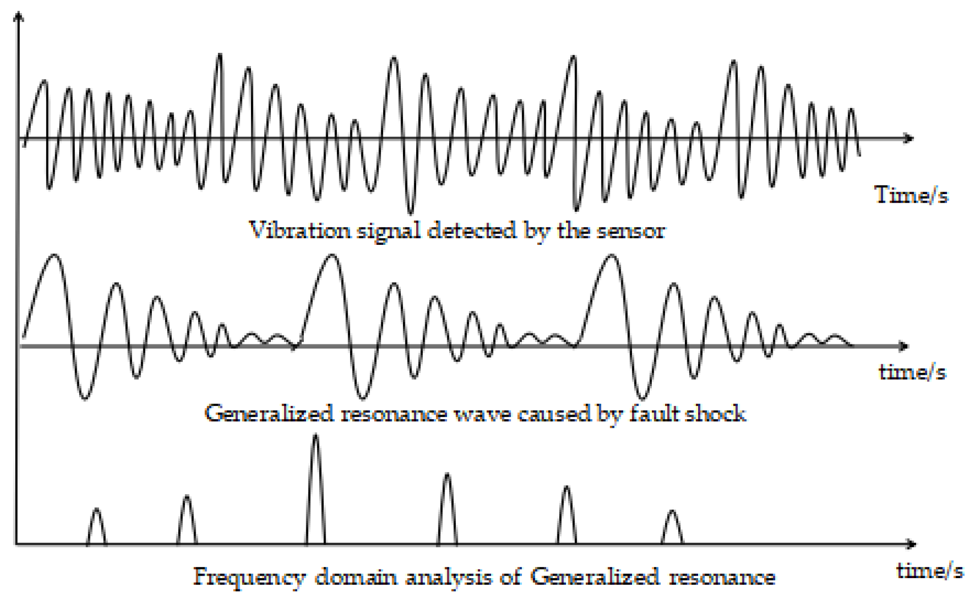
The specific process of fiber Bragg grating resonant sensor monitoring bearing is as follows: when a partial failure occurs on the surface of a certain component of the bearing, it will collide with the surface of other components during the loaded operation. This produces a concentrated shock pulse force. The sensor absorbs shock energy to generate a generalized resonance wave, and releases energy at the sensor’s own high-frequency natural frequency. After processing the high-frequency resonance wave, a vibration waveform that eliminates low-frequency vibration interference but is rich in fault information can be obtained. The vibration signal in this process is measured by the fiber Bragg grating. The fiber Bragg grating converts the vibration signal into the axial strain of the fiber Bragg grating, and then uses the high-speed fiber Bragg grating demodulator to obtain the center wavelength of the fiber Bragg grating. By monitoring the wavelength dynamics of the fiber Bragg grating change, the bearing vibration can be monitored [29,30]. The process of picking up weak faults is shown in Figure 2.

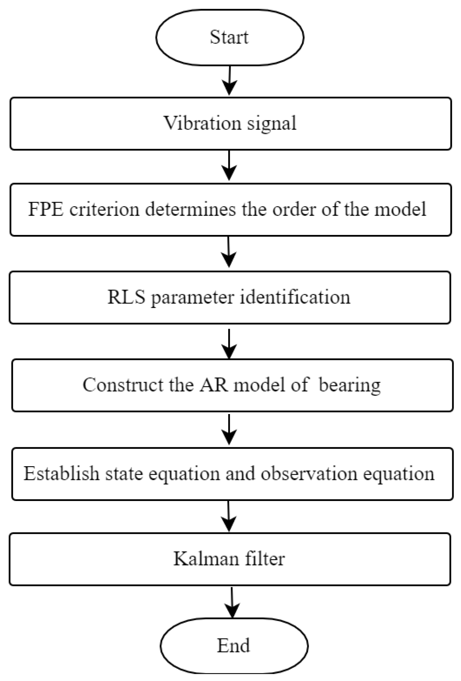
Due to the harsh working environment of the bearing, the vibration signal collected by the sensor contains a lot of noise. In order to accurately realize the detection and identification of the faulty bearing’s signal, it is necessary to reduce the noise of the vibration signal collected by the sensor. This article establishes the AR model, determines the AR model order through the FPE criterion, and then determines the AR model parameters through the RLS algorithm, and finally uses the Kalman filter to achieve noise reduction. The main process is shown in Figure 3.

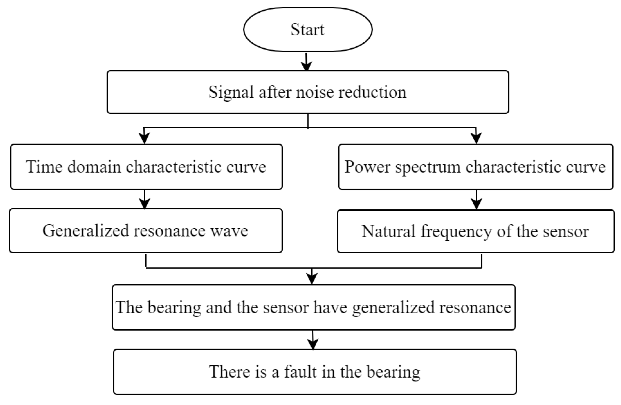
The detection process of the bearing faulty signal is as follows: first, the time-domain analysis is performed on the signal after noise reduction. If the time-domain characteristic curve has attenuated oscillation, it indicates that there is a generalized resonance wave. Then, analyze the power spectrum of the signal after noise reduction, and the extracted high frequency components is close to the natural frequency of the fiber Bragg grating resonant sensor, which further shows that the bearing and the fiber Bragg grating resonant sensor have a generalized resonance phenomenon. According to the generalized resonance principle, when there is a weak fault in the bearing, the fault will have a generalized resonance phenomenon with the fiber Bragg grating resonant sensor. Bearing fault detection can be realized by time-domain analysis and power spectrum analysis. Figure 4 shows the process.

The bearing fault identification process is as follows: improved autocorrelation envelope spectrum analysis is performed on the signal after noise reduction, the fault frequency is extracted, and the fault frequency is compared with the fault characteristic frequency of the bearing to determine the location of the bearing fault. The bearing fault identification process is shown in Figure 5.

4. Design of Faulty Bearing Experiment Platform

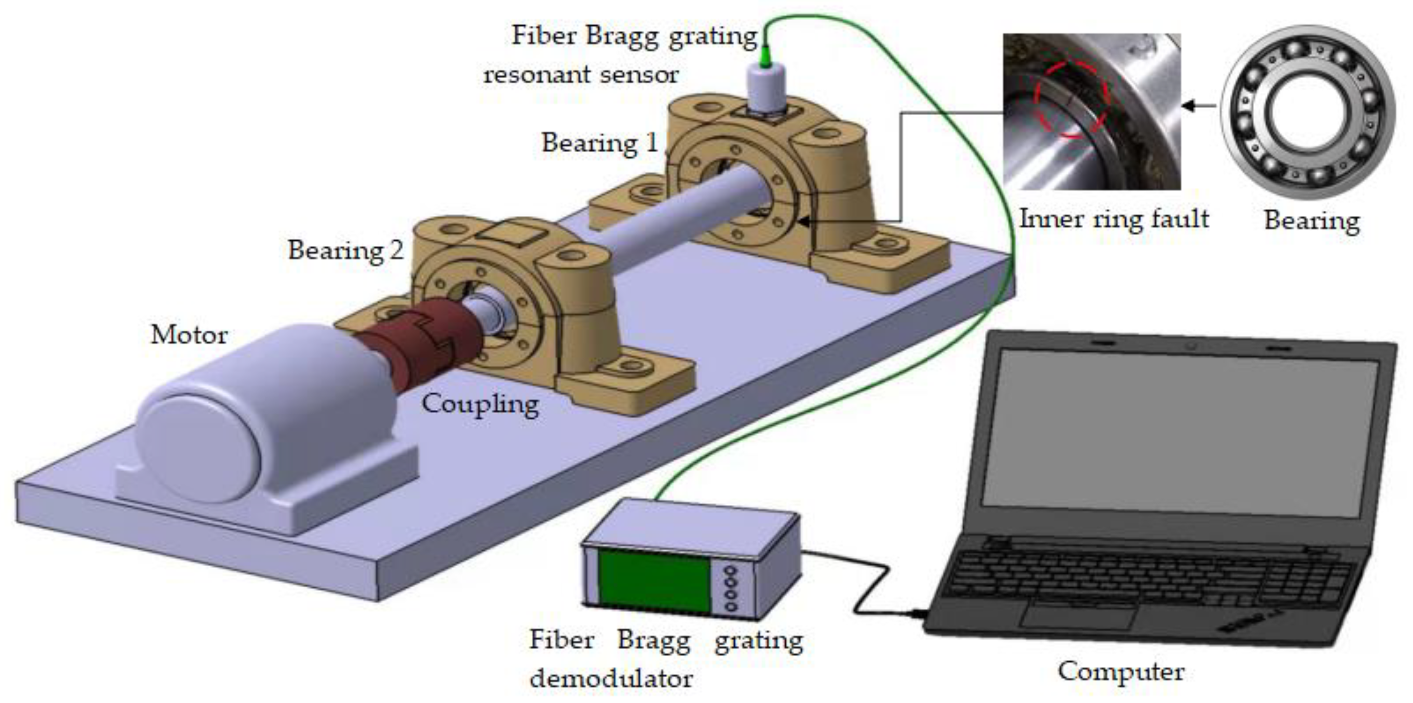
The bearing fault monitoring experiment platform is built with UG software. It mainly includes a drive motor, a coupling, a bearing 1, a bearing 2, a fiber Bragg grating resonant sensor, a fiber Bragg grating demodulator, and a computer, as shown in Figure 6.

The fiber Bragg grating resonant sensor is fixed on bearing 1 and is used to detect shock vibration signals. Bearing 1 is a test bearing, and bearing 2 is a symmetrical support bearing. The diameter of the rotating shaft at the output end of the drive motor is 20 mm. The shaft diameter is 35 mm. The coupling is used to connect the drive motor and the shaft to transmit power and buffer the excessive instantaneous speed difference. When the sensor detects the bearing vibration, the fiber Bragg grating is deformed by force. When a bearing component has a fault and a small shock occurs, the sensor absorbs the shock energy to generate a generalized resonance wave, and releases energy at the natural frequency of the sensor. The vibration signal is collected by fiber Bragg grating, and then the change of central wavelength is read by the demodulator. Finally, the collected data is analyzed by computer to diagnose whether the bearing is faulty.

Based on fiber Bragg grating resonant sensor, signal coupling caused by electromagnetic interference can be effectively avoided, and micro shock monitoring can be realized. The sensor has the advantages of high sensitivity, good stability, small volume, convenient installation, etc.

The sampling rate of the fiber Bragg grating resonant sensor is 200 KHz and the natural frequency is 6325 Hz. This frequency belongs to the high-frequency, which can effectively avoid the influence of low-frequency interference during the bearing rotation process [30].

The bearing model selected in the experiment is Harbin bearing 7307. The number of rolling elements is 8, and the contact angle is 0°. The outer ring diameter and the inner ring diameter of the bearing are 80 mm and 35 mm. The diameter of the rolling element is 14.5 mm. The pitch diameter of the bearing is 57.5 mm. The motor rotates at a constant speed and the speed is 300 rpm (5 Hz).

Substituting the bearing parameters into the formula in

Table 1. The calculation formula of bearing fault characteristic frequency.

Fault Type	Formula	Fault Characteristic Frequency
Inner Ring	$\mathrm{BPFI}/\mathrm{BPFO}=\frac{1}{2}\mathrm{Z}\left(1\pm \frac{\mathrm{d}}{\mathrm{D}}\cos \propto \right){\mathrm{f}}_{\mathrm{s}}$	25 Hz
Outer Ring	$\mathrm{BPFO}=\frac{1}{2}\mathrm{Z}\left(1-\frac{\mathrm{d}}{\mathrm{D}}\cos \propto \right){\mathrm{f}}_{\mathrm{s}}$	15 Hz
Rolling Element	$\mathrm{BSF}=\frac{\mathrm{D}}{\mathrm{d}}\left(1-{\left(\frac{\mathrm{d}}{\mathrm{D}}\right)}^2{\cos }^2\propto \right){\mathrm{f}}_{\mathrm{s}}$	18.57 Hz
Cage	$\mathrm{FTF}=\frac{1}{2}\left(1-\frac{\mathrm{d}}{\mathrm{D}}\cos \propto \right){\mathrm{f}}_{\mathrm{s}}$	1.87 Hz

, the fault characteristic frequencies of four parts can be obtained.

Table 1: Z is the number of rolling elements, $\propto$ is the angle between the force direction of the rolling element and the vertical line of the inner and outer raceways, ${\mathrm{f}}_{\mathrm{s}}$ is the rotation frequency of the bearing, $\mathrm{d}$ is the average diameter of the rolling elements, and $\mathrm{D}$ is the pitch diameter of the bearing and the spherical center distance of the two rolling elements on the same line.

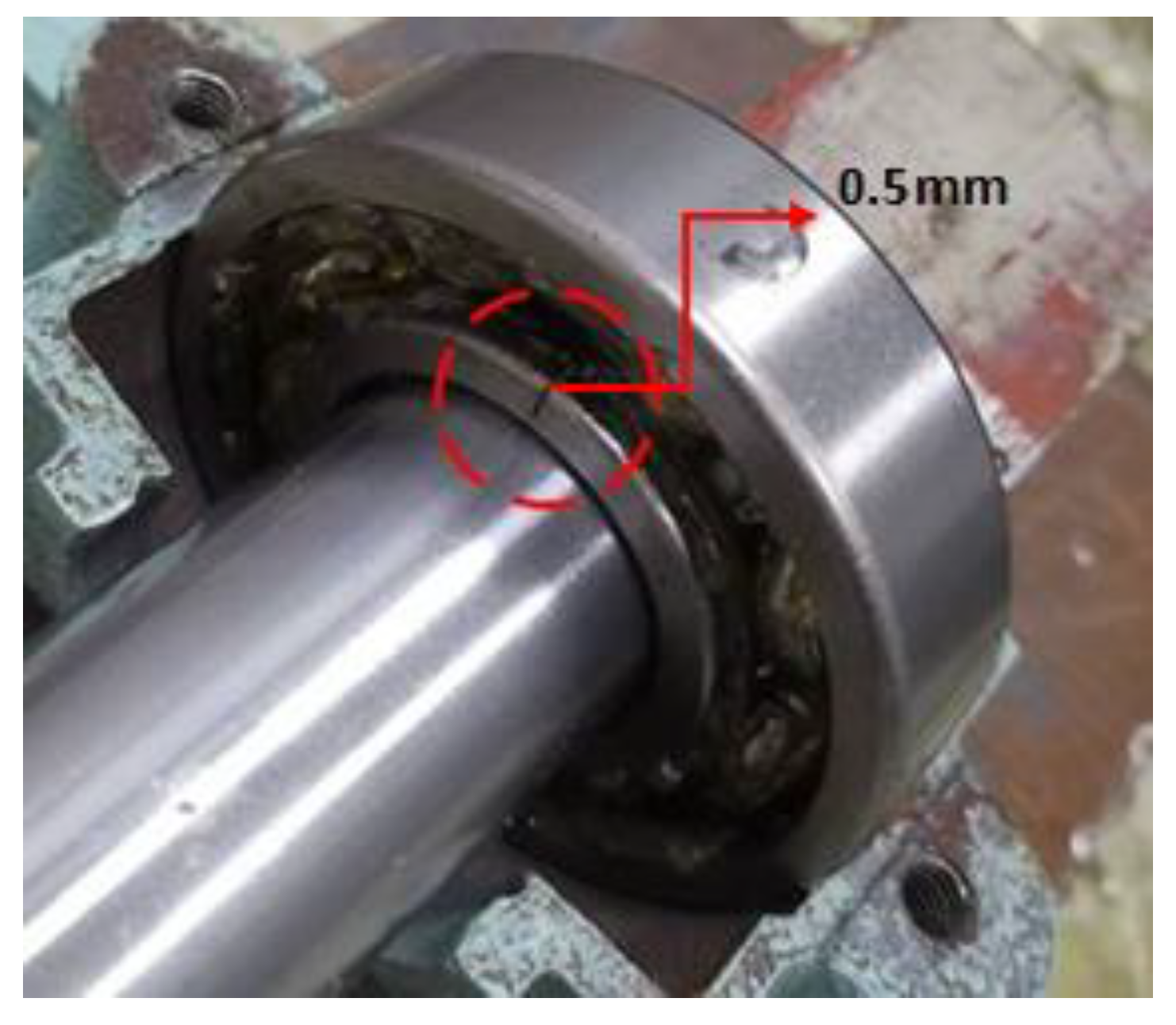
In order to simulate the fault of the bearing in actual operation, a small incision with a width of 0.5 mm is produced in the inner ring of the bearing, as shown in Figure 7.

5. Experiment Data Analysis

5.1. Determination of AR Model Order and Model Parameters of Faulty Bearing Vibration Signal

The following analysis uses MATLAB software to analyze the data. First, zero averaging and smoothing processing are performed on the original data, and then the data is analyzed according to the FPE criterion to obtain the FPE criterion function curve, as shown in Figure 8. The number of data samples is $3\times {10}^4$.

In Figure 8: As the order of the model increases, the overall trend of the FPE criterion curve is decreasing. When n is 5, the corresponding FPE criterion curve is at a lower value, and the curve decreases slowly. When n is 33, the FPE standard curve has the lowest value, the corresponding variance is the smallest, and the FPE standard curve is stable after this point.

Next, the standard deviation (SD) and mean square error (MSE) are calculated for $\mathrm{n}=5$ and $\mathrm{n}=33$, as shown in

Table 2. SD and MSE when $\mathrm{n}=5$ and $\mathrm{n}=33$.

Model Order	SD	MSE
$5$	0.0635	0.0355
33	0.0558	0.0355

. When $\mathrm{n}=5$ and $\mathrm{n}=33$, the SD is close and the MSE is same.

In the AR model, the higher order of the model will improve the accuracy of the estimation, but it will also increase the computational burden, and false peaks or false details will be generated in the power spectrum estimation. Combining the data in Table 2, the model order of this article is chosen to be n = 5.

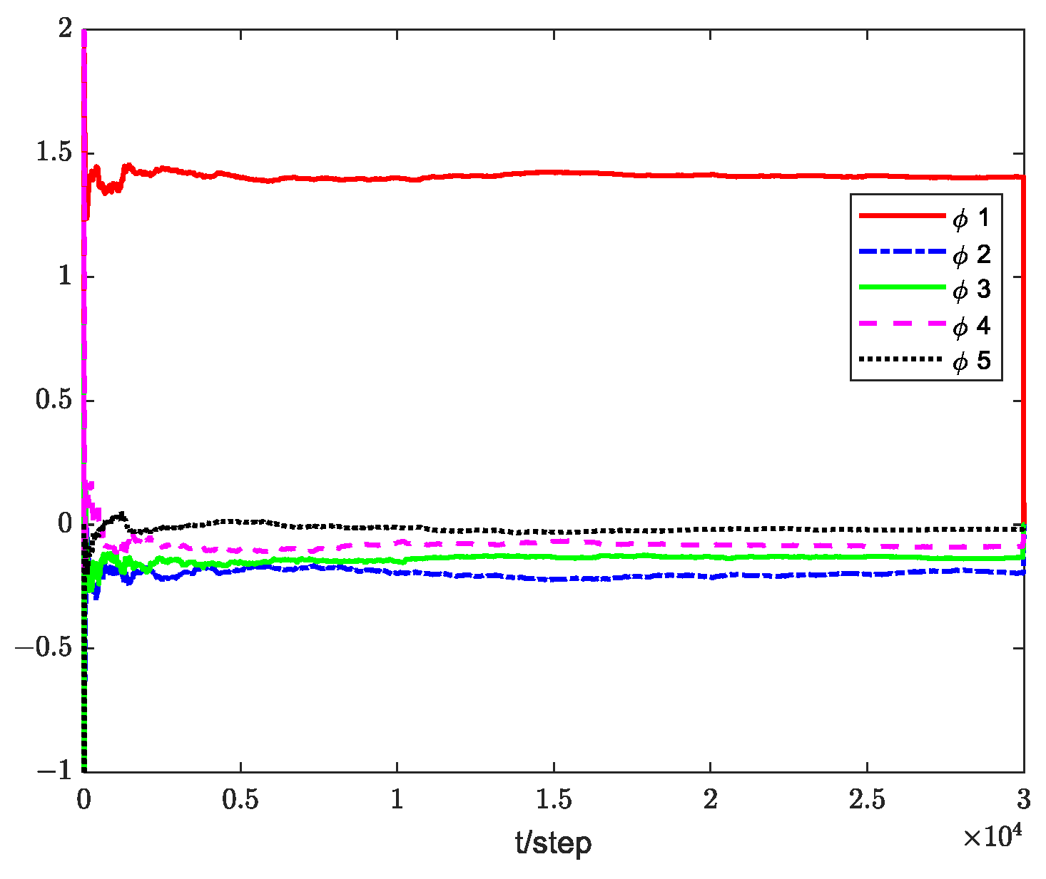
According to the RLS identification algorithm, the AR model parameters are determined. The parameters ${\mathsf{\phi }}_1,{ \mathsf{\phi }}_2,{ \mathsf{\phi }}_3,{\mathsf{\phi }}_4,{ \mathsf{\phi }}_5$ have convergence and the values are 1.4209, −0.2045, −0.1405, −0.0694, −0.0371. The identification result of parameters are shown in Figure 9.

According to the established AR model, its autocorrelation function is obtained, and the autocorrelation function has tailing, as shown in Figure 10.

5.2. Bearing Vibration Signal Analysis and Bearing Fault Detection and Diagnosis

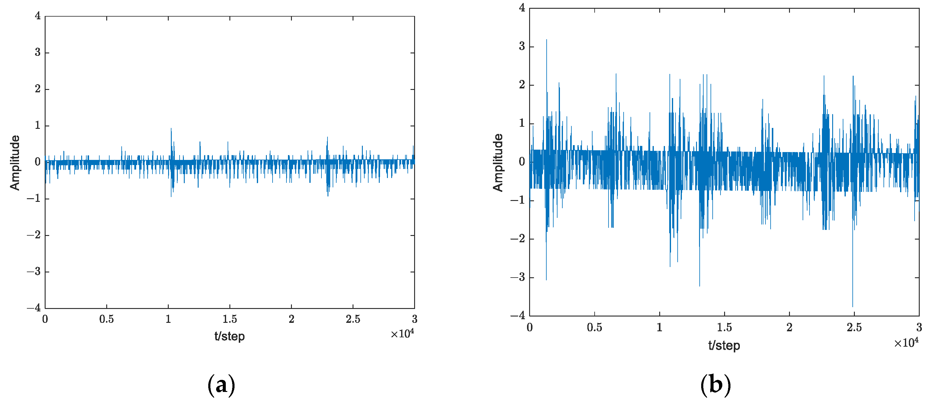
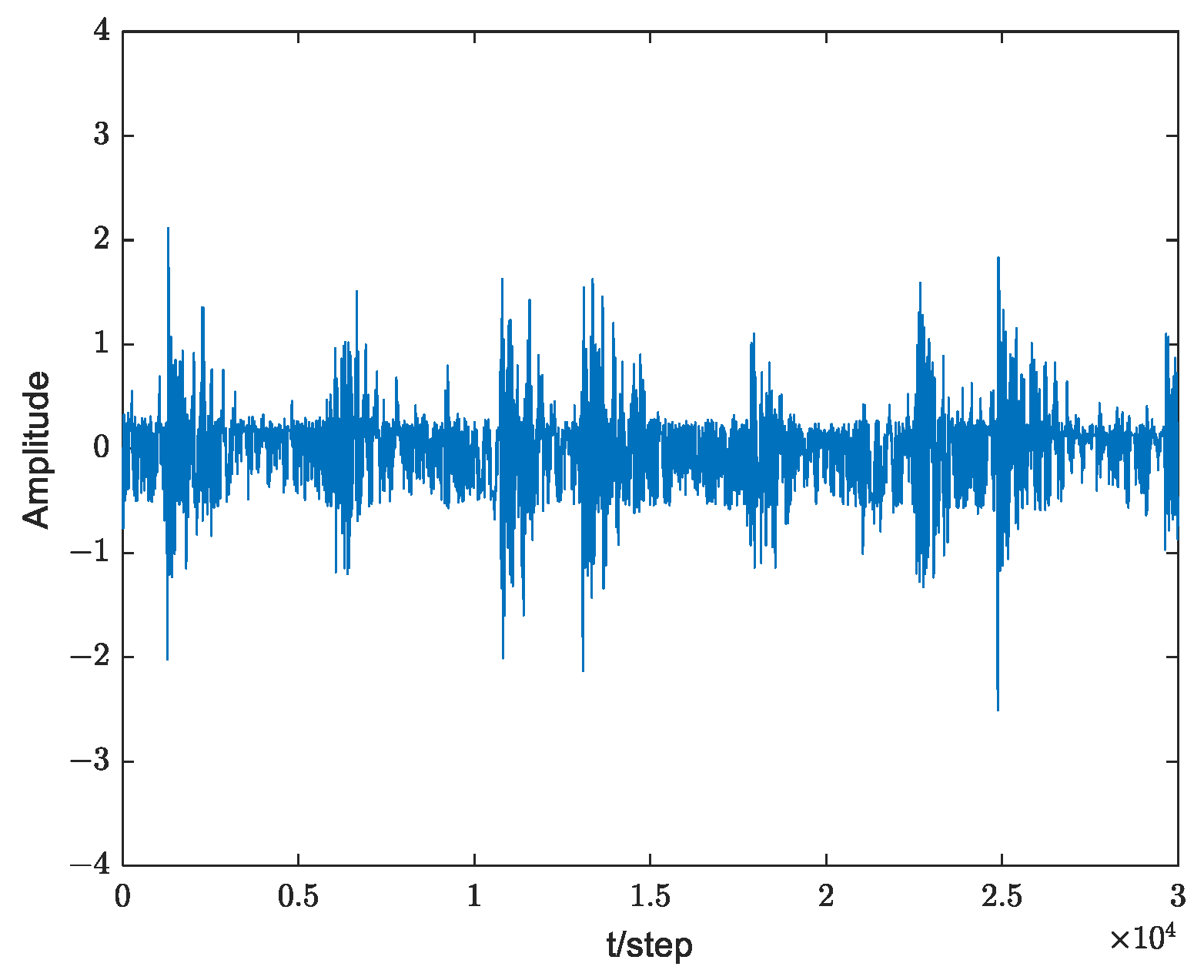
The normal bearing vibration signal and the faulty bearing vibration signal are shown in Figure 11. The vibration signal of the normal bearing is relatively stable, and the vibration signal of the faulty bearing has obvious fluctuations. It is difficult to directly determine the location of the bearing fault from the faulty bearing vibration signal.

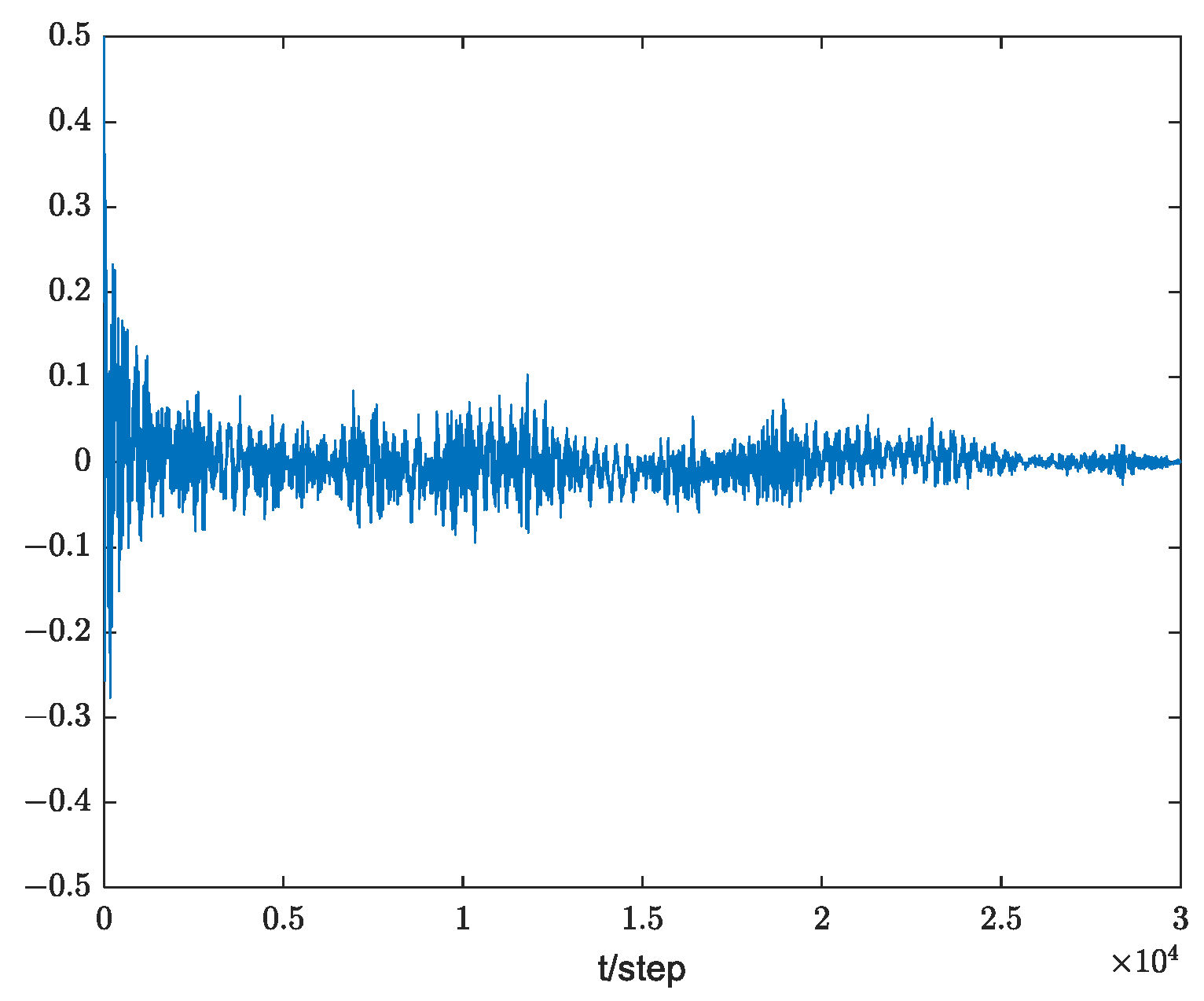
Because the bearing will produce different degrees of vibration when it is running, the vibration signal usually contains noise components and other interference information, resulting in the bearing fault signal shock characteristic’s being not obvious, and affected by external interference. In the case of excessive external interference, the fault feature is often submerged. In addition, when an incipient fault occurs in the bearing, the amplitude of the fault component relative to the frequency of rotation and other components irrelevant to the fault is smaller. In order to accurately diagnose the fault of the bearing, it is necessary to perform noise reduction pretreatment on the bearing vibration signal. Figure 12 shows the state of the bearing after Kalman filter.

Analysis of Figure 11b and Figure 12 shows that the vibration signal after Kalman filter noise reduction maintains the state of the original vibration signal.

The signal after Kalman filter noise reduction has an obvious free damping oscillation process. In order to clearly observe the attenuated oscillation signal, the time domain signal of the first 10,000 points is selected in Figure 13. It is clear from the analysis that the weak vibration generated by the bearing fault and the fiber Bragg grating resonant sensor has generalized resonance, and a generalized resonance wave is generated.

The following analyses are the power spectrum analysis of the vibration signals of the normal bearing and the faulty bearing. If there is a high frequency component around 6325 Hz in the power spectrum, it means that there is a fault in the bearing. The faulty bearing resonates with the sensor, releasing energy at the sensor’s natural frequency [30].

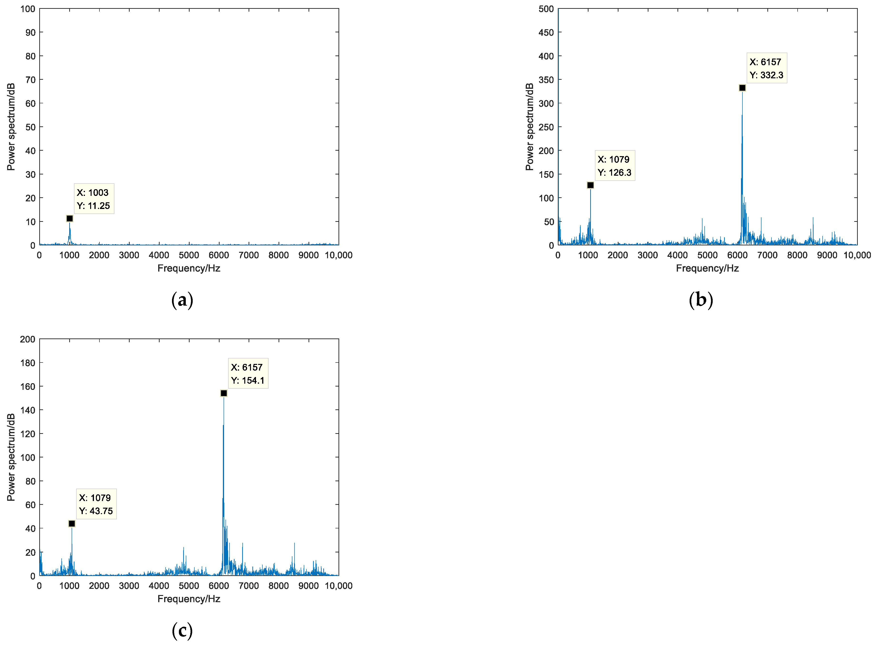
The power spectrum analysis of the normal bearing’s vibration signal, the faulty bearing’s vibration signal and the vibration signal after noise reduction by the Kalman filter are shown in Figure 14. The three power spectrums in Figure 14a–c contain low frequency components of 1003 Hz, 1079 Hz and 1079 Hz respectively. These low frequency values do not affect the diagnosis of bearing faults.

When the frequency value in the power spectrum is close to the natural frequency of the fiber Bragg grating resonance sensor at 6325 Hz, it indicates that the bearing is faulty, and the fault is in resonance with the sensor. In Figure 14b,c, the power spectrum of fault bearing signal includes a 6157 Hz high-frequency component, which is close to the natural frequency of the sensor. From this frequency, it can be determined that the bearing is faulty. Additionally, the extracted components of the filtered power spectrum are the same, without spectral distortion. Figure 14a There is no high-frequency component in the normal bearing signal power spectrum.

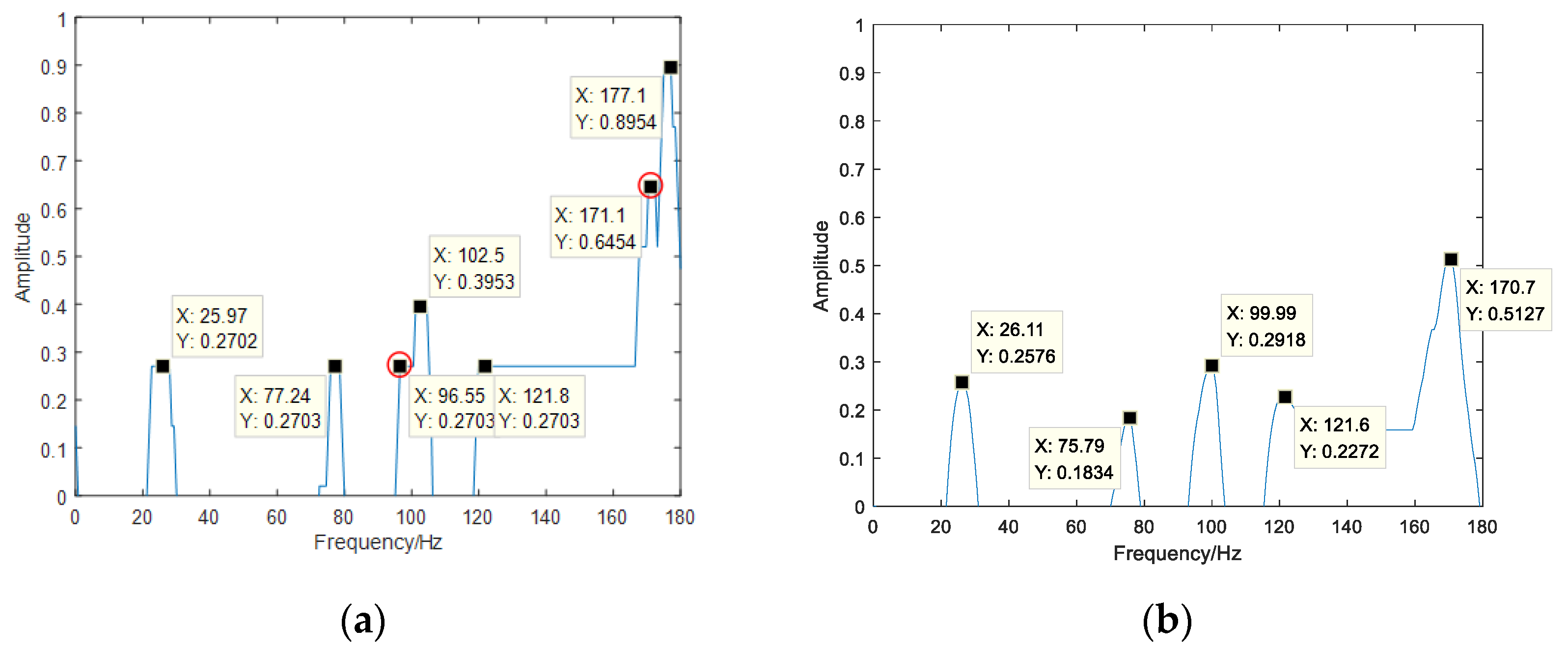
The following is the envelope spectrum analysis of the faulty bearing vibration signal, as shown in Figure 15. Combined with the theoretical value of the bearing fault characteristic frequency in Table 1, f_IR = 25 Hz. In Figure 15a, the frequency components are 25.97 Hz, 77.24 Hz, 102.5 Hz, 121.8 Hz, 177.1 Hz. These frequencies are multiples of the inner ring fault characteristic frequency, respectively, are f_IR, 3f_IR, 4f_IR, 5f_IR, 7f_IR. It can be diagnosed that the bearing fault occurs in the inner ring. Among them, 96.55 Hz, 171.1 Hz are the interference frequencies, which have been marked with a red circle.

Figure 15b is the envelope analysis of the signal after the Kalman filter. The frequency components included are 26.11 Hz, 75.79 Hz, 99.99 Hz, 121.6 Hz, 170.7 Hz. The above frequency components are the inner ring fault characteristic frequency f_IR, 3f_IR, 4f_IR, 5f_IR, 7f_IR.

According to the analysis of Figure 15, the disadvantages of envelope analysis are as follows:

(1)

If the working background of the bearing is noisy and the ambient noise is large, there will be more envelope components obtained through envelope analysis. It is easy to cause the fault signal envelope to be mixed with the noise envelope, and it is not easy to distinguish.

(2)

The envelope of the fault characteristic frequency is not obvious. The largest envelope in the envelope spectrum corresponds to the 7f_IR frequency of the bearing fault characteristic frequency. The analysis of the envelope is required to determine the bearing fault location.

Comparing Figure 15a,b, after Kalman filter noise reduction, the obtained envelope spectrum has the following advantages:

(1)

There is no noise envelope in the envelope spectrum. The obtained envelopes are all multipliers of the fault characteristic frequency.

(2)

The envelope spectrum curve is smooth without any slight noise interference.

The following is the analysis of autocorrelation envelope spectrum, as shown in Figure 16.

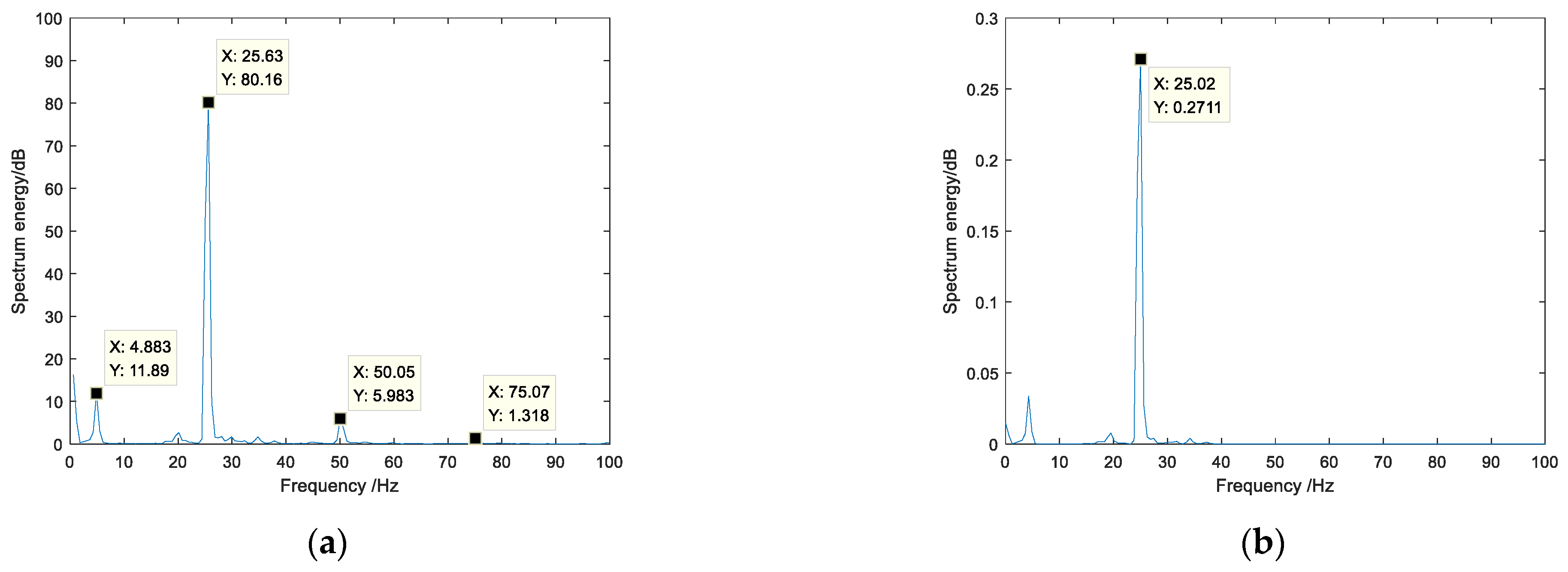
As visible in Figure 16a, in the improved autocorrelation envelope power spectrum, the bearing fault frequency and double frequency 25.63 Hz, 50.05 Hz, 75.07 Hz can be extracted, and the bearing rotation frequency 4.883 Hz can also be extracted.

Compared with Figure 15b, the fault characteristic frequency is obvious, and the corresponding amplitude is the largest. The envelope spectrum is concise, does not contain more frequency components, and is easy to distinguish from other noise components.

Figure 16b is the autocorrelation envelope power spectrum by the literature [31]. Compared with Figure 16a, Figure 16a can not only directly extract the bearing fault characteristic frequency, but also extract other frequency components. From this, the accuracy of the extracted fault frequency can be further proved.

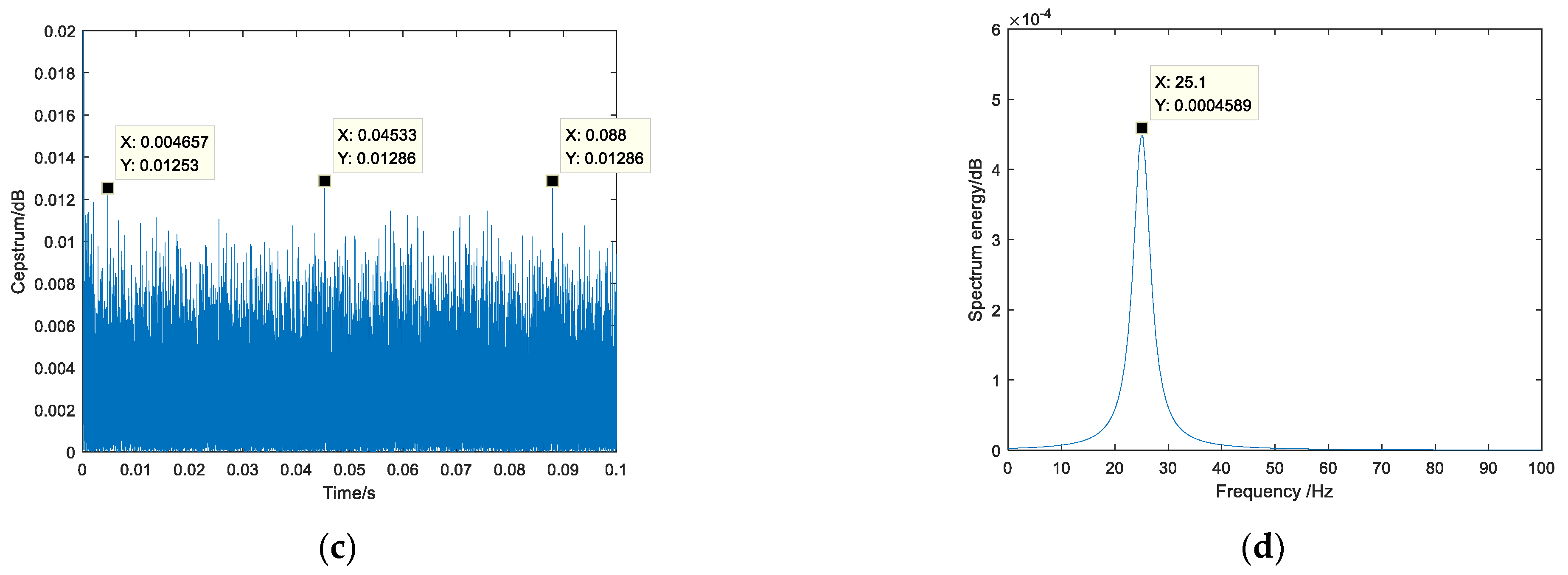
The cepstral analysis method adopted by the literature [32] is shown in Figure 16c. In Figure 16c, the x-axis is the time domain, and the peak value appears every 0.04 s. From this, it can be determined that there is a periodic frequency, which is 25 Hz.

The analyses in Figure 16a,c can both extract the characteristic frequencies of bearing faults. Comparing the two methods, the advantage of the improved autocorrelation envelope power spectrum analysis method is that the extracted fault frequencies are intuitive and do not require further analysis. The cepstrum contains too much noise and is easily disturbed by noise, and further analysis is required to obtain the fault frequency.

As seen in Figure 16d, in the autocorrelation envelope maximum entropy spectrum, the characteristic frequencies of bearing faults are directly extracted without interference frequencies.

Through the above analysis, the method based on Kalman filter and spectrum analysis can effectively realize the detection and identification of the faulty bearing.

5.3. Compare with Existing Method

(1)

Compare with wavelet transform

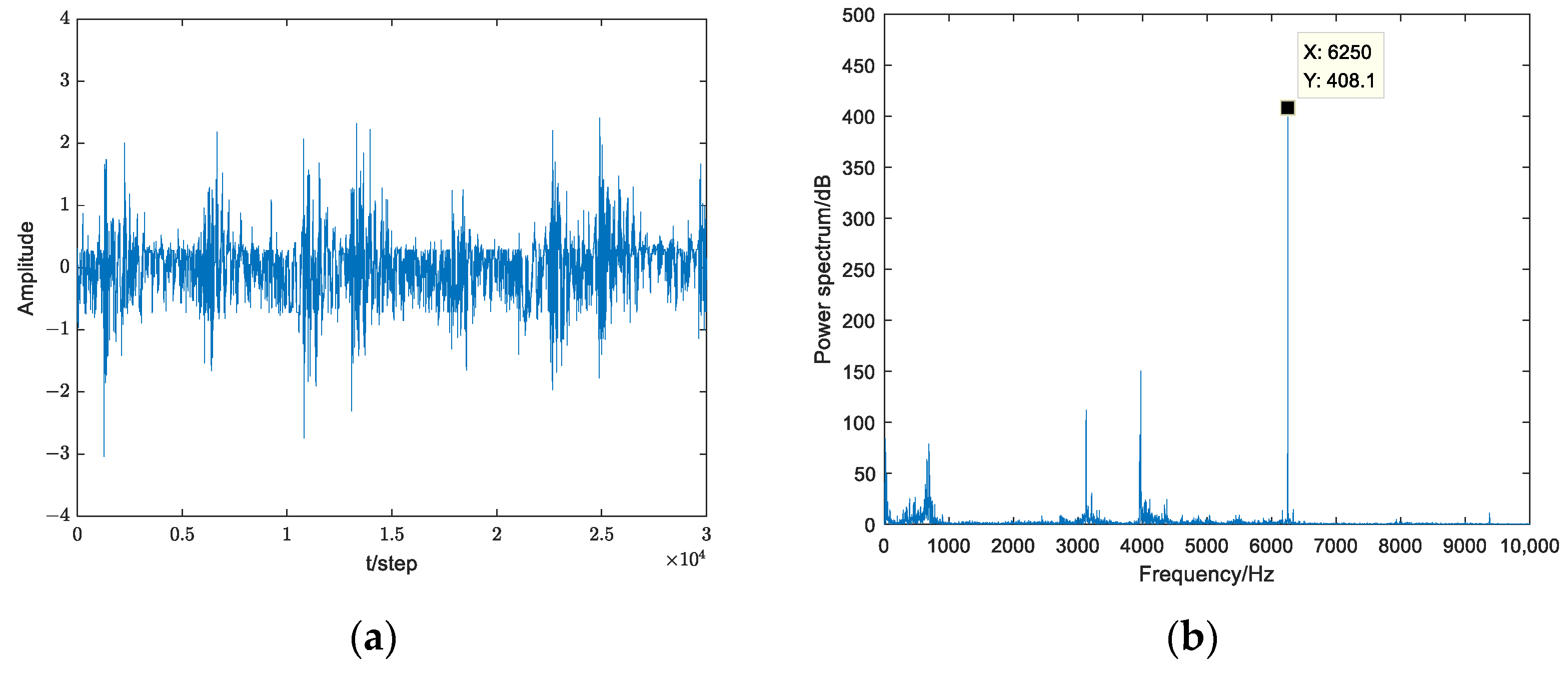
Wavelet transform is a common and effective method in extracting weak signals. The wavelet transform decomposes the signal into the scale domain, and through multi-resolution decomposition, the weak signal components in the original signal become prominent. First of all, the bearing vibration signal is decomposed and reconstructed by 11 layers using Haar wavelet. The reconstructed signal is shown in Figure 17a. The recombined signal is then subjected to power spectrum analysis, as shown in Figure 17b.

Analyzing Figure 17a and Figure 11b, one can see that the time-domain diagram after wavelet transform recombination is deviated from the time-domain diagram of the original signal. The time-domain image reorganized by wavelet transform cannot fully reflect the vibration state. Analyzing the power spectrum of the wavelet-recombined signal of Figure 17b, there is a high frequency component of 6250 Hz, which shows that wavelet transform can realize the detection of bearing faults. Comparing Figure 17b with Figure 14c, it can be obtained that when the wavelet transform’s recombined signal is analyzed for power spectrum, high-frequency components can be extracted, but the extraction of low-frequency components is not accurate.

(2)

Compare with empirical mode decomposition

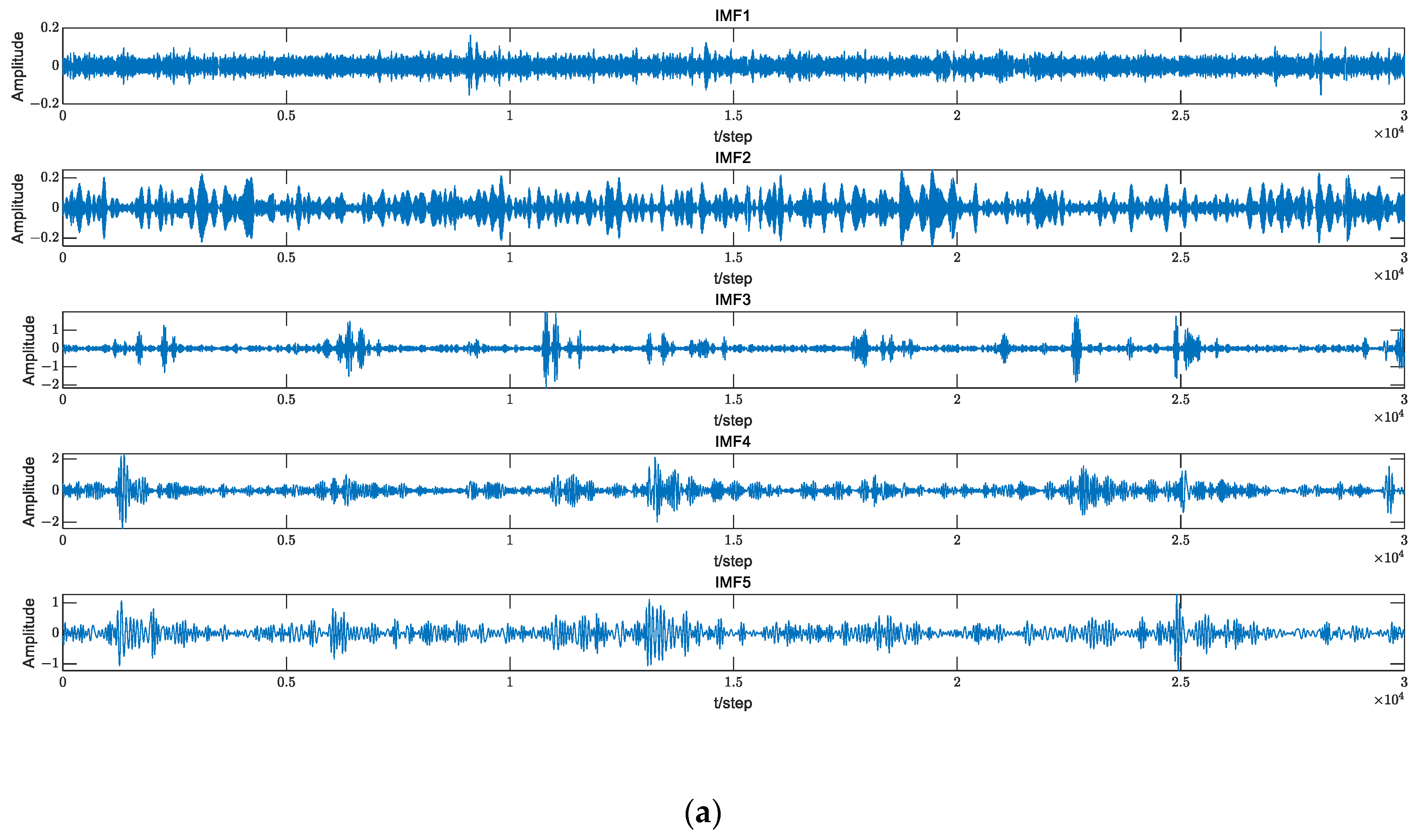
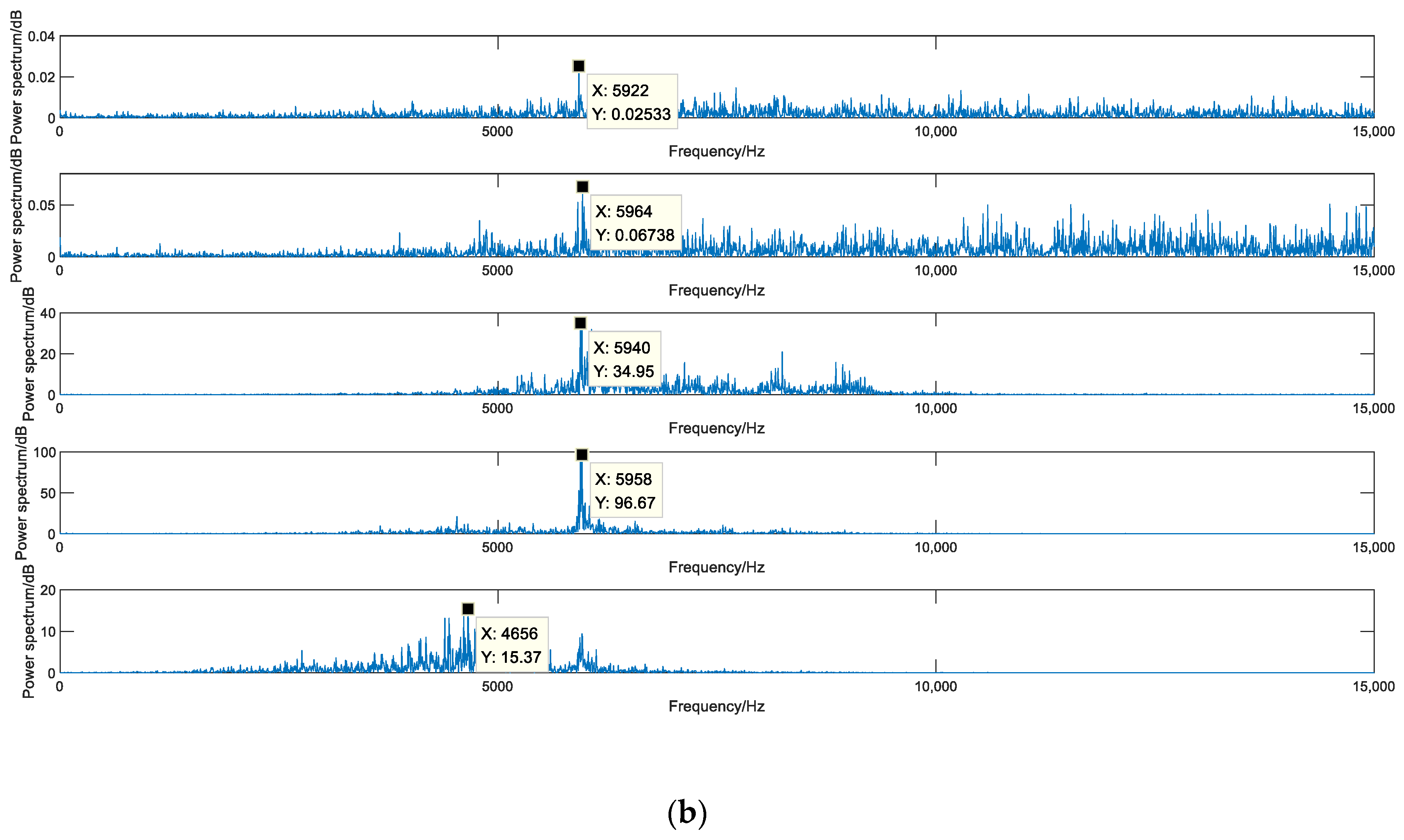
Empirical mode decomposition (EMD) is often used to extract weak faults of bearings. It can decompose complex signals into a limited number of intrinsic mode functions. The decomposed IMF components contain local characteristic signals of different time scales of the original signal. The bearing signal is decomposed by EMD. The time-domain signal and spectrum of 1–5 IMFs are shown in Figure 18.

According to Figure 18, time-domain signals of different IMFs are obtained through EMD decomposition. Different IMFs have different power spectrum. Among them, the power spectrum frequency of IMF4 is the purest, with little noise interference. The peak value is 5958 Hz, which is closing to the natural frequency of the sensor. Compared with Figure 14c, the maximum frequency in the power spectrum obtained after Kalman filter is 6157 Hz, which is close to the natural frequency of the sensor 6325 Hz.

Finally, the signal to noise ratio (SNR) and root mean square error (RMSE) are analyzed, as shown in

Table 3. Noise reduction signal quality evaluation index.

Noise Reduction Method	SNR	RMSE
Kalman filter	5.6302	0.3833
Wavelet transform	1.7621	0.3925
Empirical mode decomposition	1.7039	0.5095

.

The SNR value represents the ratio of the effective signal energy to the noise energy in the signal. The higher the value, the smaller the value of noise mixed in the signal. The RMSE value reflects the difference between the signal after noise reduction and the original signal. The lower the value, the closer the signal after noise reduction is to the original signal.

According to the data in Table 3, the noise reduction effect of the Kalman filter is better than that of wavelet transform and Empirical mode decomposition.

6. Analysis of Bearing Fault Signal of Case Western Reserve University

The bearing fault signals of Case Western Reserve University in the United States are analyzed by this article method. In an experimental device the 1.5 kW 3-phase induction motor is connected to a power meter and a torque sensor through a self-calibrating coupling, and is operated by a driving fan.

The vibration signal is collected by the acceleration sensor and installed on the bearing seat with a magnetic seat. The sampling frequency is 12,000 Hz, and the number of sampling points is 8192. The rolling bearing is SKF6205-2RS JEM deep groove ball bearing. Single point fault is found on the surface of inner ring and outer ring respectively by electro discharge machining, which is then run at constant speed for motor loads of 1 horsepower. The size of faults is 0.18 mm in diameter and 0.28 mm in depth. The rotation frequency fr of the shaft is 1772 rpm (29.53 Hz). According to the literature [33], the inner ring fault frequency is 5.415 fr (159.9 Hz), and the outer ring fault frequency is 3.585 fr (105.9 Hz).

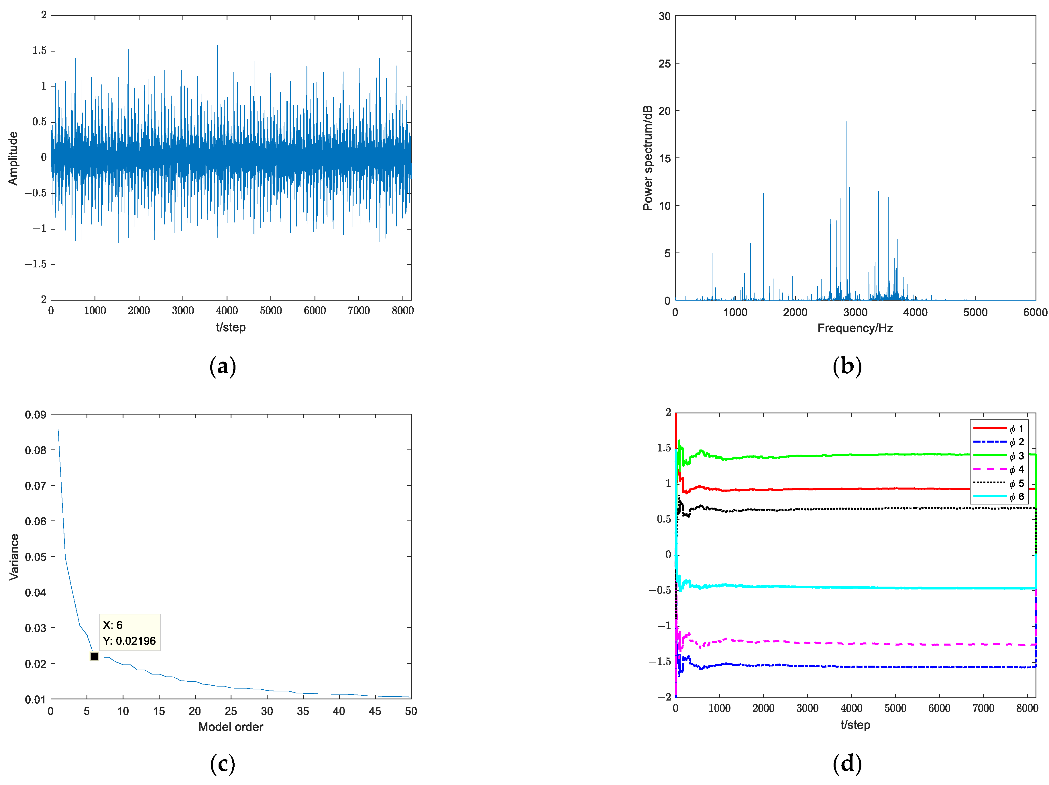
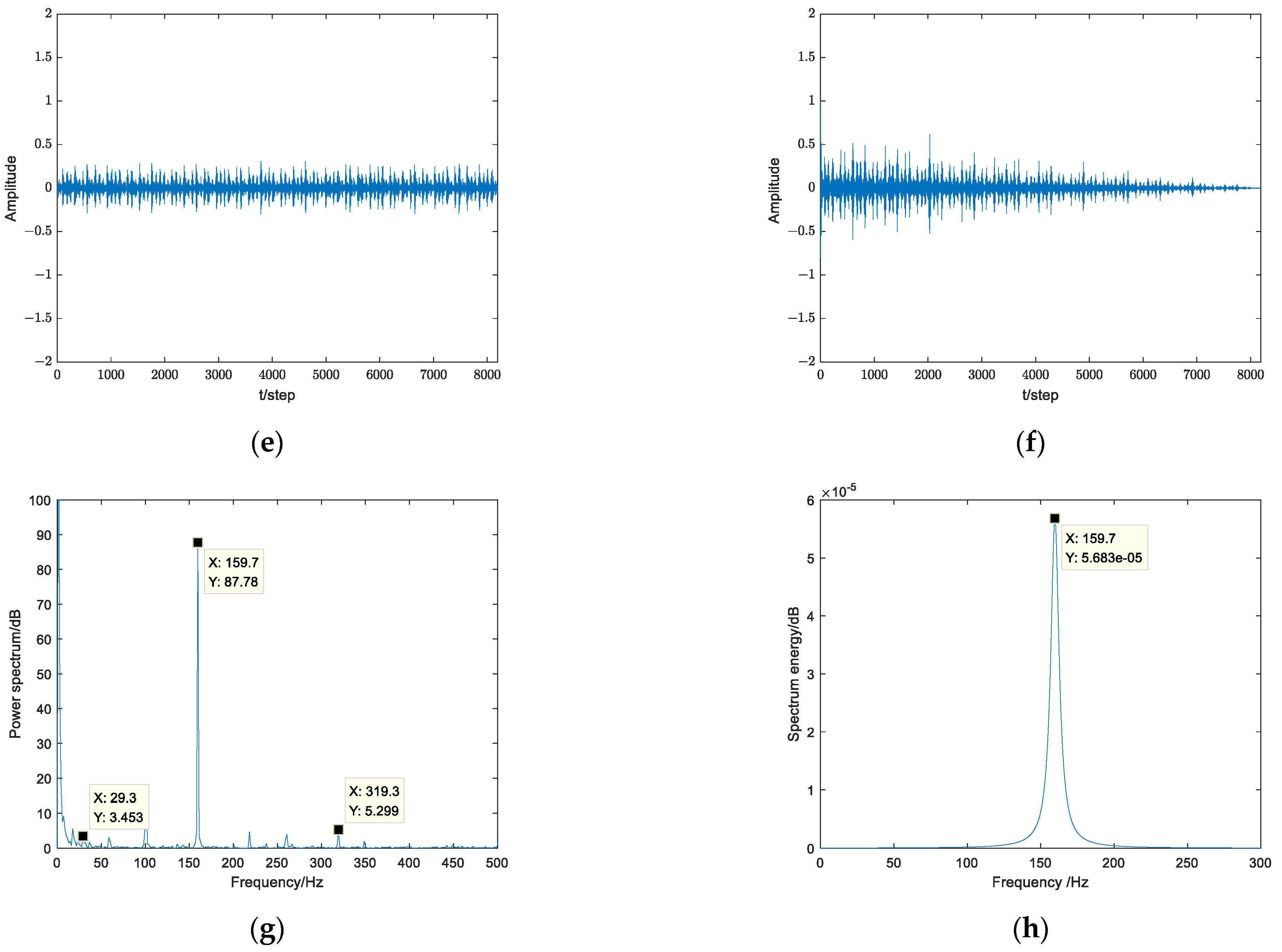
The fault signal of the bearing inner ring and its power spectrum are shown in Figure 19a,b. The AR model is established based on the vibration signal of inner ring, and the model order is 6, as shown in Figure 19c. The model parameters have convergence, respectively 0.9335, −1.5689, 1.4184, −1.2555, 0.6631, −0.4627, as shown in Figure 19d. The signal after the Kalman filter is shown in Figure 19e. The autocorrelation function has tailing, as shown in Figure 19f. The SNR after filtering is 9.1874. An improved autocorrelation envelope power spectrum, 159.7 Hz and 319.3 Hz correspond to the inner ring fault frequency and its multiple frequency, and 29.3 Hz corresponds to the shaft frequency, as shown in Figure 19g. The maximum amplitude extracted by autocorrelation envelope maximum entropy spectrum corresponds to the fault frequency of bearing inner ring, as shown in Figure 19h.

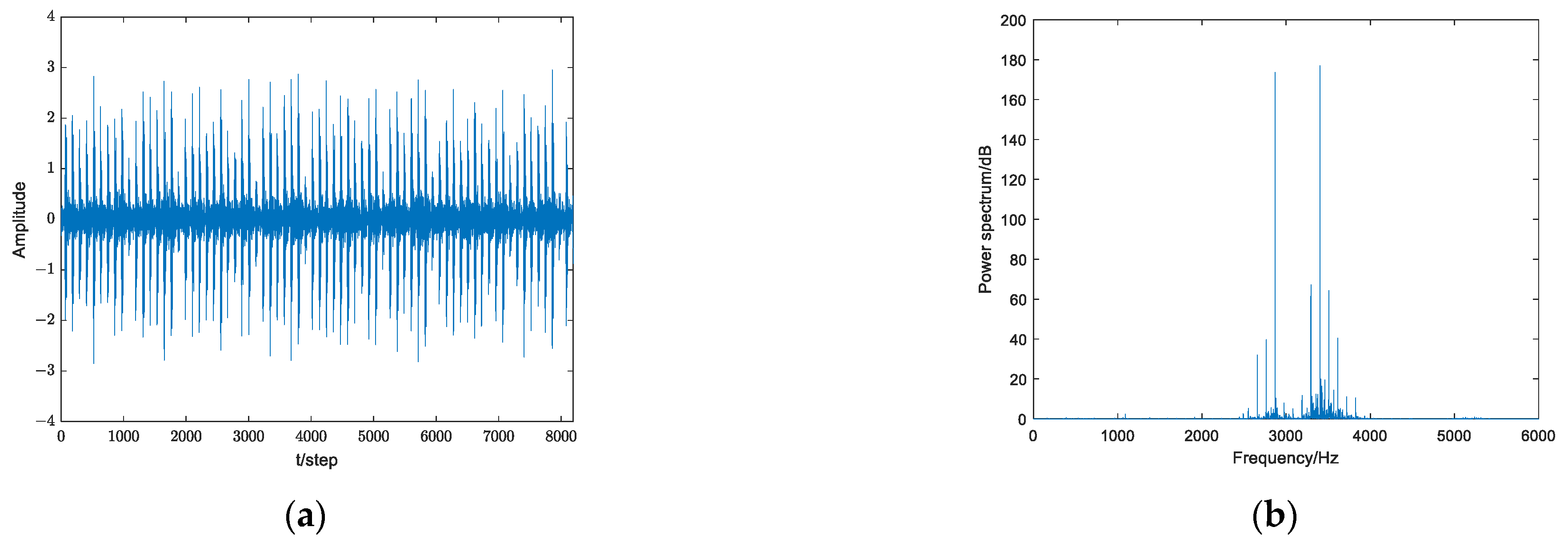
The fault signal of the bearing outer ring is obvious, and the time domain signal and its power spectrum are shown in Figure 20a,b. AR model order is 5, as shown in Figure 20c. Model parameters are −0.1491, −1.1965, 0.1153, −0.3152, 0.1179, as shown in Figure 20d. The signal after the Kalman filter is shown in Figure 20e. The autocorrelation function has tailing, as shown in Figure 20f. The SNR after filtering is 16.3518. Improved autocorrelation envelope power spectrum, 106.9 Hz, 212.4 Hz, 319.3 Hz, 424.8 Hz correspond to the outer ring fault frequency and its multiple frequency, and 29.3 Hz corresponds to the shaft frequency, as shown in Figure 20g. The maximum amplitude extracted by autocorrelation envelope maximum entropy spectrum corresponds to the fault frequency of the bearing outer ring, as shown in Figure 20h.

7. Conclusions

In view of the fact that the fault signal of the bearing is weak, and the detection and diagnosis are difficult, the fiber Bragg grating generalized resonant sensor is used to realize the monitoring of the inner ring fault vibration signal. Combined with the vibration monitoring signal, the state space model is established. The FPE criterion and RLS algorithm are used to determine the model order and model parameters. After establishing a faulty bearing dynamic system, the Kalman filter is used for signal noise reduction processing, and power spectrum analysis is combined with improved autocorrelation envelope spectrum analysis to detect and identify weak bearing faults. This verifies the effectiveness and feasibility of the resonance detection method based on the Kalman filter and spectrum analysis for rolling bearing fault signals. Compared with other methods, the proposed improved autocorrelation envelope spectrum analysis method can better identify the characteristic frequencies of bearing faults. The subsequent research after this article might investigate other effective methods for detection and diagnosis of bearing faults, and the problem of detection and identification of multiple simultaneous bearing faults.

References

1. Xiao, L.; Zhang, X.; Lu, S.; Xia, T.; Xi, L. A novel weak-fault detection technique for rolling element bearing based on vibrational resonance. J. Sound Vib. 2019, 438, 490–505. [Google Scholar] [CrossRef]
2. Hou, B.; Wang, D.; Chen, Y.; Wang, H.; Peng, Z. Interpretable online updated weights: Optimized square envelope spectrum for machine condition monitoring and fault diagnosis. Mech. Syst. Signal Process. 2022, 109, 108779. [Google Scholar] [CrossRef]
3. Abhilash, S.; Pradeep, R.; Rejith, R.; Bijudas, C. Health monitoring of rolling element bearings using improved wavelet cross spectrum technique and support vector machines. Tribol. Int. 2021, 154, 106650. [Google Scholar]
4. Randall, R.; Antoni, J. Rolling element bearing diagnostics-A tutorial. Mech. Syst. Signal Process. 2011, 25, 485–520. [Google Scholar] [CrossRef]
5. Li, C.; Sánchez, V.; Zurita, G.; Lozada, M.; Cabrera, D. Rolling element bearing defect detection using the generalized synchrosqueezing transform guided by time–frequency ridge enhancement. ISA Trans. 2016, 60, 274–284. [Google Scholar] [CrossRef]
6. Ahmadi, A.; Petersen, D.; Howard, C. A nonlinear dynamic vibration model of defective bearings—The importance of modelling the finite size of rolling elements. Mech. Syst. Signal Process. 2015, 52–53, 309–326. [Google Scholar] [CrossRef]
7. Gupta, P.; Pradhan, M. Fault detection analysis in rolling element bearing: A review. Mater. Today 2017, 4, 2085–2094. [Google Scholar] [CrossRef]
8. Djebala, A.; Ouelaa, N.; Hamzaoui, N. Detection of rolling bearing defects using discrete wavelet analysis. Meccanica 2008, 43, 339–348. [Google Scholar] [CrossRef]
9. Wang, H.; Chen, J.; Dong, G. Feature extraction of rolling bearing’s early weak fault based on EEMD and tunable Q-factor wavelet transform. Mech. Syst. Signal Process. 2014, 48, 103–119. [Google Scholar] [CrossRef]
10. Jiang, R.; Chen, J.; Dong, G.; Liu, T.; Xiao, W. The weak fault diagnosis and condition monitoring of rolling element bearing using minimum entropy deconvolution and envelop spectrum. Proc. Inst. Mech. Eng. 2013, 227, 1116–1129. [Google Scholar] [CrossRef]
11. Yao, R.; Jiang, H.; Li, X.; Gao, J. Bearing incipient fault feature extraction using adaptive period matching enhanced sparse representation. Mech. Syst. Signal Process. 2021, 166, 108467. [Google Scholar] [CrossRef]
12. Wang, S.; Niu, P.; Guo, Y.; Wang, F.; Li, W. Early diagnosis of bearing faults using decomposition and reconstruction stochastic resonance system. Measurement 2020, 158, 107709. [Google Scholar] [CrossRef]
13. Rezazadeh, N.; De Luca, A.; Lamanna, G.; Caputo, F. Diagnosing and Balancing Approaches of Bowed Rotating Systems: A Review. Appl. Sci. 2022, 12, 9157. [Google Scholar] [CrossRef]
14. Rezazadeh, N.; Ashory, M.-R.; Fallahy, S. Identifcation of shallow cracks in rotating systems by utilizing convolutional neural networks and persistence spectrum under constant speed condition. J. Mech. Eng. Autom. Control Syst. 2021, 2, 135–147. [Google Scholar] [CrossRef]
15. Rezazadeh, N.; De Luca, A.; Perfetto, D. Unbalanced, cracked, and misaligned rotating machines: A comparison between classification procedures throughout the steady-state operation. J. Braz. Soc. Mech. Sci. Eng. 2022, 44, 450. [Google Scholar] [CrossRef]
16. Sawalhi, N.; Wang, W.; Becker, A. Vibration signal processing for spall size estimation in rolling element bearings using autoregressive inverse filtration combined with bearing signal synchronous averaging. Adv. Mech. Eng. 2017, 9, 1687814017703007. [Google Scholar] [CrossRef] [Green Version]
17. Bastami, A.; Vahid, S. Estimating the size of naturally generated defects in the outer ring and roller of a tapered roller bearing based on autoregressive model combined with envelope analysis and discrete wavelet transform. Measurement 2020, 159, 107767. [Google Scholar] [CrossRef]
18. Wu, Y.; Jiang, B.; Wang, W. Incipient winding fault detection and diagnosis for squirrel-cage induction motors equipped on CRH trains. ISA Trans. 2020, 99, 488–495. [Google Scholar] [CrossRef]
19. Borghesani, P.; Smith, W.; Randall, R.; Antoni, J.; Badaoui, M.; Peng, Z. Bearing signal models and their effect on bearing diagnostics. Mech. Syst. Signal Process. 2022, 174, 109077. [Google Scholar] [CrossRef]
20. Kumar, J.; Chauhan, P.; Pandit, P. Time domain vibration analysis techniques for conditiion monitoring of rolling element bearing: A review. Mater. Today 2022, 62, 6336–6340. [Google Scholar]
21. Deng, Z.; Wang, X.; Gao, Y. Modeling and Estimation; Science Press: Beijing, China, 2016. [Google Scholar]
22. Sun, S.; Deng, Z. Multi-sensor optimal information fusion Kalman filter. Automatica 2004, 40, 1017–1023. [Google Scholar] [CrossRef]
23. Sun, S.; Lin, H.; Ma, J.; Li, X. Multi-sensor distributed fusion estimation with applications in networked systems: A review paper. Inf. Fusion 2017, 38, 122–134. [Google Scholar] [CrossRef]
24. Dolenc, B.; Boškoski, P.; Juričić, D. Distributed bearing fault diagnosis based on vibration analysis. Mech. Syst. Signal Process. 2016, 66–67, 521–532. [Google Scholar] [CrossRef]
25. Chen, B.; Cheng, Y.; Zhang, W.; Gu, F. Enhanced bearing fault diagnosis using integral envelope spectrum from spectral coherence normalized with feature energy. Measurement 2022, 189, 110448. [Google Scholar] [CrossRef]
26. Liu, J.; Xu, Y.; Pan, G. A combined acoustic and dynamic model of a defective ball bearing. J. Sound Vib. 2021, 501, 116029. [Google Scholar] [CrossRef]
27. Nayana, B.; Geethanjali, P. Analysis of statistical time-domain features effectiveness in identification of bearing defects from vibration signal. IEEE Sens. J. 2017, 17, 5618–5625. [Google Scholar] [CrossRef]
28. Sharma, V.; Parey, A. A review of gear fault diagnosis using various condition indicators. Procedia Eng. 2016, 144, 253–263. [Google Scholar] [CrossRef] [Green Version]
29. Lyu, G.; Jiang, Y.; Wang, C.; Zhao, J.; Che, G.; Jiang, X. Simulation design of fiber Bragg grating resonant sensor for train bearing damage detection. In Proceedings of the 2018 Asia Communications and Photonics Conference (ACP), Hangzhou, China, 26–29 October 2018; Volume 10, pp. 26–29. [Google Scholar]
30. Chen, X.; Jiang, Y.; Zhou, B.; Zhan, H.; Li, H.; Lyu, G.; Sun, S. Early Weak Fault Diagnosis of Rolling Bearings Based on Fiber Bragg Grating Sensing Monitoring. Symmetry 2021, 13, 1473. [Google Scholar] [CrossRef]
31. Su, W.; Wang, F.; Zhu, H.; Zhang, Z.; Guo, Z. Rolling element bearing faults diagnosis based on optimal Morlet wavelet filter and autocorrelation enhancement. Mech. Syst. Signal Process. 2010, 24, 1458–1472. [Google Scholar] [CrossRef]
32. Chen, X.; Wang, E.; Jiang, Y.; Zhao, J.; Li, H.; Lyu, G.; Sun, S. Generalized Resonance Sensor Based on Fiber Bragg Grating. Photonics 2021, 8, 156. [Google Scholar] [CrossRef]
33. Smith, W.; Randall, R. Rolling element bearing diagnostics using the Case Western Reserve University data: A benchmark study. Mech. Syst. Signal Process. 2015, 64–65, 100–131. [Google Scholar] [CrossRef]
Figure 1. Bearing fault detection and identification process.
Applsci 13 01472 g001
Figure 2. The weak fault picking-up process based on the principle of generalized resonance.
Applsci 13 01472 g002
Figure 3. Noise reduction process.
Applsci 13 01472 g003
Figure 4. Bearing fault detection process.
Applsci 13 01472 g004
Figure 5. Bearing fault identification process.
Applsci 13 01472 g005
Figure 6. Bearing fault monitoring experiment platform.
Applsci 13 01472 g006
Figure 7. Fault bearing inner ring.
Applsci 13 01472 g007
Figure 8. FPE criterion function curve.
Applsci 13 01472 g008
Figure 9. Model parameter identification curves.
Applsci 13 01472 g009
Figure 10. Autocorrelation function curve.
Applsci 13 01472 g010
Figure 11. Bearing vibration signal: (a) normal bearing vibration signal curve; (b) faulty bearing vibration signal curve.
Applsci 13 01472 g011
Figure 12. State estimation after Kalman filter.
Applsci 13 01472 g012
Figure 13. Free damped oscillation curve of the signal after Kalman filter noise reduction.
Applsci 13 01472 g013
Figure 14. Power spectrum analysis curve: (a) normal bearing power spectrum analysis curve; (b) the power spectrum analysis curve of faulty bearing vibration signal without Kalman filter noise reduction; and (c) the power spectrum analysis curve of faulty bearing vibration signal with Kalman filter noise reduction.
Applsci 13 01472 g014
Figure 15. The envelope spectrum analysis curve: (a) the envelope spectrum analysis curve of faulty bearing vibration signal without Kalman filter noise reduction; and (b) the envelope spectrum analysis curve of faulty bearing vibration signal with Kalman filter noise reduction.
Applsci 13 01472 g015
Figure 16. The analysis of autocorrelation envelope spectrum: (a) improved autocorrelation envelope power spectrum analysis; (b) autocorrelation envelope power spectrum analysis; (c) cepstral analysis; and (d) autocorrelation envelope maximum entropy spectrum analysis.
Applsci 13 01472 g016aApplsci 13 01472 g016b
Figure 17. Wavelet transform noise reduction signal analysis: (a) the time-domain curve of the reconstructed signal after wavelet decomposition; and (b) power spectrum analysis curve.
Applsci 13 01472 g017
Figure 18. Empirical mode decomposition analysis: (a) the time-domain curves of the 1–5 IMFs; and (b) the power spectrum of the 1–5 IMFs.
Applsci 13 01472 g018aApplsci 13 01472 g018b
Figure 19. Inner ring fault analysis results: (a) bearing inner ring fault signal; (b) power spectrum analysis; (c) model order; (d) model parameters; (e) signal after Kalman filter; (f) autocorrelation function curve; (g) improved autocorrelation envelope power spectrum analysis; and (h) autocorrelation envelope maximum entropy spectrum analysis.
Applsci 13 01472 g019aApplsci 13 01472 g019b
Figure 20. Outer ring fault analysis results: (a) bearing inner ring fault signal; (b) power spectrum analysis; (c) model order; (d) model parameters; (e) signal after Kalman filter; (f) autocorrelation function curve; (g) improved autocorrelation envelope power spectrum analysis; and (h) autocorrelation envelope maximum entropy spectrum analysis.
Applsci 13 01472 g020aApplsci 13 01472 g020b