A Unified Mixed Deep Neural Network for Fatigue Damage Detection in Components with Different Stress Concentrations

Abstract

The article presents a mixed deep neural network (DNN) approach for detecting micron-scale fatigue damage in high-strength polycrystalline aluminum alloys. Fatigue testing is conducted using a custom-designed apparatus integrated with a confocal microscope and a moving stage to accurately pinpoint the instance of micron-scale crack emergence. The specimens are monitored throughout the duration of the experiment using a pair of high-frequency ultrasonic transducers. The mixed DNN is trained with ultrasonic time-series data that are obtained from two sets of specimens categorized by different stress concentration factors. To understand the effects of mixing the data from both types of specimens, a parametric analysis is performed by varying the amount of training data from each specimen to develop a series of mixed DNNs. The mixed DNN, when tested on unseen data from both specimens, exhibits an accuracy of over 95%. This article, therefore, demonstrates a successful alternative to customized DNNs for new types, geometries, or stress concentration factors in the materials under consideration.

1. Introduction

Fatigue damage detection is one of the most important challenges that structural engineers encounter [1]. Although fatigue has been studied for a long time, a predictive framework to accurately and comprehensively estimate the fatigue life of a component is still elusive. This is mainly due to the massively vast parameter space that drives such failures in an operational setup [2]. Several factors, such as the load conditions, history, frequency, part geometry, presence of stress concentration factors, material microstructures, and defects, contribute to fatigue failure. While these factors may be accounted for to a certain extent through laboratory-based experiments to develop predictive models, they are often accompanied by unprecedented levels of uncertainties in operation. Hence, a comprehensive experimentation to understand their coupled effects can become overwhelmingly expensive to perform [3]. Analytical and computational modeling are often performed to augment the understanding of fatigue failures. However, owing to their computational cost, these numerical models are often carried out on reduced-scale geometries. Consequently, a quantifiable generalized framework that can predict the fatigue behavior of any new materials and manufacturing processes remains a major research focus to date [4]. A broad categorization of fatigue-related research is shown in Figure 1a. The focus is either toward a ‘prediction’ or a ‘detection’ framework. The prediction framework is mainly targeted toward influencing design criteria that can enable a fatigue-resistant component, whereas the detection framework is useful in a working environment. The studies in the prediction framework can be further divided into three main domains, viz., analytical, computational, and empirical. A recent review paper by Liao et al. [5] summarizes four classes of analytical techniques that are pursued for this problem, viz., nominal stress approaches, local stress-strain approaches, critical distance theories, and weighting control-parameter-based approaches. High-fidelity computational frameworks are being mainly developed using crystal plasticity simulations [6,7]. Empirical frameworks, the oldest and comparatively more error-prone among the three, have been documented through several design criteria [8]. The detection framework on the other hand, is targeted toward developing better sensing mechanisms [9] or improving the data analysis therein [10]. The detection framework provides real-time information about a component’s health and, therefore, is critical in ensuring the safe operation of fatigue-critical components in operation [11].

The elemental philosophy of the sensor-based approach is underpinned by the sensors’ ability to continuously stream data that has the health information of a component encoded in it. By analyzing this stream of data via data-driven approaches, reliable strategies can be developed to detect fatigue damage in real-time [12]. Over the past few decades, rapid growth of deep learning methodologies has ushered a new era in damage detection analysis algorithms [10,13,14,15,16]. As summarized by Zhao et al. [15], the state-of-the-art deep learning methods, such as autoencoders, restricted Boltzmann machines, deep Boltzmann machines, convolutional neural nets (CNNs), and recurrent neural nets (RNNs), have shown promising applications to this field. CNNs have shown a particular proclivity to problems that have dealt with imaging datasets [14,16]. However, in the majority of complex structures, such as aerospace or automobiles, the reliance is solely on time-series-based sensors, which can be processed with varied methods. For instance, through an autoencoder, acoustic emission data were analyzed to localize damage [17]. With Bayesian Graph Neural Nets, Mylonas et al. [18] demonstrated the application of strain gauge sensors. Amiri et al. [19] studied damage detection in spot welds using ultrasonics and artificial neural nets (ANNs). Similarly, Bansode and Billore [20] used ANNs to study fatigue failures in rotary shafts.

Dharmadhikari et al. showed the excellence of deep neural networks (DNNs) for fatigue crack detection in notched specimens using ultrasonics [21]. Along similar lines, Amiri et al. [19], Xu et al. [22] used ultrasonics to study damage detection. In addition to a direct application of such sensors, computational assistance in guided wave-based damage detection has also been studied with neural nets [23,24]. However, much of the existing research has focused on damage detection of specimens having a fixed geometry, as shown in Figure 1b. It is well known that notches create localized stress concentrations that may significantly alter failure mechanisms. Since DNNs are trained with a huge amount of data, a logical follow-up question is: would a similar volume of training data be needed for any new specimen type? This question becomes even more paramount if the specimens are built with new manufacturing processes (e.g., additive manufacturing [25]) or expensive materials (e.g., nickel-based Rhenium containing superalloys [26]). In trying to find a solution to these challenges, if a DNN trained in some other material systems or geometries aids in any way, it would result in huge cost savings. Although there are transfer learning approaches to answer such problems [27], they often result in individual models for each specimen geometry and, therefore, may lead to an intractable number of trained models. While these questions are rather firsts-of-their-kinds in the applied mechanics field, they are not new in other domains, such as natural language processing [28].

A common theme among the language research problems is to develop a unified natural language processing framework for sparsely available language data (such as Urdu or Tibetan) from similar yet vastly available counterparts (such as Hindi or Mandarin) using a mixed learning strategy that can be schematically represented through Figure 1c. Based on the success of this framework in translating a representative phrase from any language to the other, it is hypothesized that a single machine-learning framework can also be developed for fatigue damage detection across different specimen geometries. There can be several ways to design specimens with different geometry. In the structural engineering community, the effects of stress concentration have been studied for a long time and have led to well-defined theories for commonly occurring materials and geometries [3]. This article focuses on understanding the applications of mixed learning to specimens distinguished by stress concentration factors (Figure 1a,b).

Two different stress concentration factors ($K_t$) are considered. The specimens are built from Al7075-T6, an aluminum alloy that is extensively used in aerospace applications. A custom-built fatigue testing apparatus is used to generate the required time-series data during the entire duration of the tests using ultrasonic sensors. The tests provide crack detection at a very early stage (∼45% fatigue life) owing to the use of a high-resolution confocal microscope. Baseline deep neural nets (DNNs), trained individually for each $K_t$, show above 95% accuracy. A unified DNN model is developed by mixing the data from both $K_t\mathrm{s}$ and training a single network. The unified model shows accuracies similar to the baseline DNNs, indicating the success of the unified model through the mixed learning process. To understand the impacts of the data contributions from both $K_t\mathrm{s}$, a parametric analysis is conducted by varying the contribution from each $K_t$. Incredibly, with just 10% training data from both datasets, the performance of the mixed DNN approaches close to 92% accuracy, showing its aptitude for success with scarce data for components with new materials or manufacturing processes.

The article is divided into five sections, including the present one. Section 2 summarizes the experimental protocol, followed by a data analysis methodology in Section 3. Section 4 presents the results and discussion, and Section 5 presents the conclusions and future work.

2. Experimental Method

This section reports the description and methods of the experimental procedure to validate the theoretical results.

2.1. Specimen Design

Figure 2 depicts the specimen designs following the ASTM E466 standard [29] used in this study. The specimens are made of high-strength Al7075-T6 alloy that meets the ASTM B209 standard [30]. The specimens are designed to have a one-sided stress concentration factor ($K_t$) to allow for controlled initiation of fatigue cracks for imaging purposes. Several specimen geometries are simulated using Solidworks and eventually, two geometries yielding $K_t$s of 7.1 and 8 are down-selected. For brevity, the specimens having $K_t$ of 7.1 are attributed as $K_{t1}$ and the specimens having $K_t$ of 8 are attributed as $K_{t2}$. Both sets of specimens, owing to their distinct $K_t$ values, will exhibit different failure lives. A higher $K_t$ implies larger localized stress fields. These fields can be easily computed through a finite element simulation, as shown in Figure 3. The figures depict the stresses in both notches for a tensile load of 2 kN. The simulations are performed using a Linear Elastic Isotropic model with an elastic modulus of 72 GPa, and a Poisson’s ratio of 0.33. These differences ultimately impact the instance of crack detection and the fatigue lives of the specimens, as observed in Figure 4. $K_{t2}$, with a more damaging impact, lowers the fatigue life and accelerates the crack appearance instance as compared to $K_{t1}$. The instance of crack detection (or appearance) corresponds to a crack opening displacement of 3 $\mathsf{\mu }$m [21], as detected by the confocal microscope. An elaborate description of the assistance of the confocal microscope in these experiments is presented later in Section 3.2.

2.2. Fatigue Testing

The experimental protocol has been described in detail by [21,31,32,33] and is briefly summarized in the present work. Figure 5a,b depict the fatigue testing apparatus. The apparatus is made up of four parts: (i) MTS testing equipment, (ii) a confocal microscope mounted on a moving stage, (iii) a moving stage, and (iv) ultrasonic sensors. The MTS testing equipment is a 25 kN servo-hydraulic setup. The specimens are mounted on the apparatus using custom grips and are subjected to tensile-tensile fatigue loading with a mean load of 3 kN and a stress ratio (min. stress/max. stress) of 0.5 at 20 Hz. Data are collected on a regular basis during the test using the confocal microscope and ultrasonic sensors. The tests are conducted through an MTS controller using an automated routine from the Multi-Purpose TestWare software suite.

The placement of the ultrasonic transmitter and receiver utilized during the fatigue test is kept constant at 10 mm for all experiments. The sensors used in the current study are obtained from Olympus (Shinjuku, Japan) and have a base frequency of 10 MHz, and are sampled at 100 MHz while using a pulse-echo scheme. The sensor data are in the form of a time series. In addition to ultrasonic sensors, the specimens are also monitored through a confocal microscope that is focused on the inside surface of the high-stress concentration region where fatigue cracks are likely to originate [34].

2.3. Ultrasonic Signals

A total of 15 specimens each for both $K_t$s are tested using the aforementioned experimental protocol. During the experiments, ultrasonic signals are continuously recorded until the specimen fails. For both the $K_t$s, roughly 30,000 individual signals are collected per specimen leading to a vast volume of data. When these signals are concatenated together sequentially, a visible attenuation is observed, as shown in Figure 6a,b for both specimens. An insight into the nature of the individual signals is shown through zoomed-in plots at three windows (named 1, 2, and 3). A representative concatenation of three individual signals is also shown for all three windows in Figure 6a. Each one of these individual signals is for one data point. The first window depicts a healthy signal, followed by an attenuated version in the second window. The third window is mainly noise, indicating that the specimen has developed a significantly large crack to obstruct the ultrasonic transmission path. At this juncture, there are two major points that need to be addressed to define the problem proposed in this article. First, although signal attenuation is clearly evident while moving towards failure, the exact instance of crack appearance cannot be determined solely with ultrasonic signals. Additional information is needed to corroborate the failure. Secondly, there seems to be no visual difference between the two signals in Figure 6a,b to differentiate between $K_t$s. There is a difference in the nature and amplitudes of the pulses. However, that is merely an experimental artifact and not an indication of any $K_t$.

2.4. Binary Classification Using the Confocal Microscope

The confocal microscope is focused on the location of high stress, shown through a schematic in Figure 7a. This orientation enables the microscope to access the entire region where the stress is likely to be higher (Figure 7b). During the experiment, through continuous monitoring, the microscope can identify the exact instance of the emergence of a crack in the fatigue damage process. Figure 7c depicts a portion of the high-stress region in a healthy state. The detection of a crack is shown in Figure 7d. Making use of the high-resolution capability [34], this instance of crack detection with the confocal microscope corresponds to a crack opening displacement of 3 $\mathsf{\mu }$m. With further loading, the crack continues to grow, as is evident in the images in Figure 7e. The objective of this research is to study the capability of crack detection at the earliest stage (Figure 7d). By mapping this information of crack emergence to the ultrasonic signals, a clear bifurcation between a healthy and a cracked state can be established.

Accordingly, the two ultrasonic signals from Figure 6 are now shown with healthy and cracked labels in Figure 8, and similar labeling is performed for the data from all the specimens.

Table 1. Data distribution among the two classes for both $K_t$s.

Specimen Type	Total Data	Healthy Data	Cracked Data
$K_{t1}$	448,939	204,571	244,368
$K_{t2}$	458,655	196,175	262,480

shows the exact amount of signals collected for each $K_t$ in addition to the relative distribution among the healthy and cracked classes. The signals, while traveling through any material, are impacted by the varied local stress fields, as shown in Figure 3. These differences are created due to the stress concentration factors and, in turn, have their signatures embedded into the ultrasonic signals. Hence, although the signals look virtually similar, the bifurcation between the healthy and cracked states would be heavily dependent on $K_t$s. By virtually similar, the authors imply that the individual signals from both the specimens have three peaks, as indicated in window #1 in Figure 6a; the difference in relative magnitudes of these three peaks is not an indication of the specimen geometry but an experimentally induced random behavior. These observations, thereby, motivate the pursuit of a damage detection methodology that can have a unified basis to identify cracks irrespective of the $K_t$.

3. Data Analysis Methodology

Figure 9 broadly compares the mixed learning framework to a traditional (separate DNN for each $K_t$) approach. Figure 9a shows the commonplace DNN training and testing approaches observed in ref. [21] where a DNN is trained for a particular problem (or $K_t$). In the long run, this may create a hurdle due to the vast number of $K_t$s that can demonstrate minute changes. Mixed learning, as shown in Figure 9, tackles this problem by showing a method to create a single DNN that can adapt to multiple $K_t$s without any modifications. The following paragraphs elaborate on a step-by-step procedure that leads to mixed learning.

3.1. Dataset Bifurcation Strategy, Training of Baseline DNNs, and Transductive Analysis

The first step of training any DNN is to create a training and testing split of the available data from both $K_t$s (i.e., $K_{t1}$ and $K_{t2}$), as shown in Figure 10a. Although fairly common in all machine learning analyses, the distribution of this split is often ad-hoc (80–20% in this case) and is based on an intelligent estimate of the problem. The reason to explicitly mention this step is to emphasize the subsequent parametric analysis that delves into understanding the effects of such data splits. At this stage, however, following the train–test split, a separate DNN (Figure 10b) is trained and tested for each $K_t$ to create a baseline for further performance comparison. The DNN is represented using a consistent nomenclature $DN{N}_{Train:XX}^{Test:YY}$ where $XX$ and $YY$ represent the training and testing data used for the analysis, respectively. For example, the baseline DNN for $K_{t2}$ (denoted as $DN{N}_{Train:80K_{t2}}^{Test:20K_{t2}}$) is trained using 80% of the available data and tested on the remaining 20%. The DNN has a fully connected structure with seven dense hidden layers and one dense output layer with a single neuron. The network receives raw, unprocessed signal data as its input. The hidden layers use the ReLU (Rectified Linear Unit) activation function [35], while the output layer uses a sigmoid activation function [35]. The model is inspired by the encoder-decoder architecture [35], where inputs are compressed to a 2D latent space and then expanded again to reconstruct the original input. A low-dimensional latent space created due to such a structure can help in interpreting the behavior of the DNN in future studies. Logistic regression [35] is carried out on the reconstructed output. Since the task is a mutually exclusive binary classification problem, binary cross-entropy [35] is used as the loss function.

The hyperparameters for the model, i.e., the number of neurons for each hidden layer and the learning rate, are selected through a grid-search algorithm using KerasTuner [36] to ensure the optimality in terms of accuracy and speed of convergence. The optimum network (Figure 10b) has 428, 132, 96, 2, 96, 132, and 428 neurons in the seven layers, with a learning rate of 0.0004 for the Adam optimizer [36]. The fully-connected DNN architecture is shown in Figure 10c. The vast volume of data ensures that the computation rarely encounters over-fitting, and hence techniques such as $L_2$ regularization and dropouts have not been used in this model. Following the construction of these baseline DNNs, their pre-trained capabilities are tested on data from another $K_t$ without any training. $DN{N}_{Train:80K_{t1}}^{Test:20K_{t2}}$ and $DN{N}_{Train:80K_{t2}}^{Test:20K_{t1}}$, therefore, evaluates the universal applicability of pretrained DNNs ($DN{N}_{Train:80K_{t1}}$ and $DN{N}_{Train:80K_{t2}}$) across different stress concentration factors, as shown in Figure 10d. Such an analysis is also termed as ‘transductive’ analysis in the machine learning literature.

3.2. The Mixed Learning Approach

$DN{N}_{Train:80K_{t1}}$ and $DN{N}_{Train:80K_{t2}}$ demonstrate that each $K_t$ may need a customized DNN using the traditional supervised machine learning tools. This is not a sustainable solution in the long run due to the multitude of DNNs that would be needed for different $K_t$s [8]. Therefore, in an attempt to avoid the generation of individual DNNs, the mixed learning approach pools in the data from multiple sources to train a single network. As shown in Figure 11, the training data from $K_{t1}$ and $K_{t2}$ are used together to train a single DNN denoted by $DN{N}_{Train:80K_{t1}+80K_{t2}}$. In doing so, the network is trained to invariably work on both datasets without the need for a $K_t$ identification label.

The mixed DNN is trained to understand these properties through its multi-layered and fully connected network. Although the procedure remains fairly straightforward, the novel applications to fatigue damage detection engender several questions that need to be thoroughly studied. Specifically, the implications of varying the amount of data from both $K_t$s can prove to be beneficial to the structural engineering community that often deals with data and testing limitations. For instance, new materials or expensive manufacturing techniques have limited testing information. Under such circumstances, can an accurate damage detection model be built with such mixed learning? How much data is essential to have a reliable DNN for damage detection? To answer such questions, the mixed DNN is further probed with a parametric analysis by varying the training data from both $K_t$s. A generalized behavior of the mixed DNN is thereby studied by using $DN{N}_{Train:\alpha K_{t1}+\beta K_{t2}}^{Test:(100-\alpha )K_{t1}}$ and $DN{N}_{Train:\alpha K_{t1}+\beta K_{t2}}^{Test:(100-\beta )K_{t2}}$ where $\alpha$ and $\beta$ represent the training data volume variation from 10% to 80%. Since low data can possibly lead to unreliable, underfitted models, the training–testing split followed in this analysis is such that models trained with a lower percentage of the training data are tested on a higher percentage of testing data. In this way, the reliability of the models is also ensured.

Note that, in summary, all DNNs are built with the objective of identifying the health of a specimen by just looking at the ultrasonic signals. To achieve this target, a ground truth needs to be established between the healthy and cracked signals. Since these ultrasonic signals (and sensors) are not capable of segregating healthy signals from cracked ones, a confocal microscope is used as an additional information source. The confocal microscope provides the instant at which a crack emerges. During each fatigue test, all signal data acquired after this instant are labeled as cracked. The labeled data from all the specimens are then pooled together, and a training–testing data split is created. The training data are used to train the DNNs, and the testing data (which are previously unseen) are used to evaluate the capability of the DNNs in correctly distinguishing the healthy and cracked signals. This methodology, therefore, attempts to emulate a real scenario where a lab-trained and confocal-aided DNN is deployed to identify a crack by just processing an ultrasonic signal.

3.3. Performance Metrics

Since the goal of all DNNs discussed in this paper is binary classification, their performance is best represented using a confusion matrix [36] that visualizes the capability of the classifier in accurately predicting a healthy or a cracked signal. In general, the confusion matrix helps in computing three quantifiable metrics, viz., the sensitivity (true positive rate), specificity (true negative rate), and accuracy (average of sensitivity and specificity). As a corollary to the typical positive–negative terminology used in machine learning literature, a positive occurrence in this situation is equivalent to the cracked state, and a negative occurrence corresponds to a healthy state. Accordingly, sensitivity is the percentage of correctly diagnosing the data labeled as cracked, and specificity is the percentage of recognizing healthy data. It is imperative for all DNNs to have high sensitivity in this damage detection problem, particularly in safety-critical environments. This ensures the reliable detection of cracked components. High overall accuracy is indicative of a good all-round performance in identifying both classes of data.

4. Results and Discussion

4.1. Performance of the Baseline DNNs and Transductive Analysis

The individual performance of the baseline DNNs ($DN{N}_{Train:80K_{t1}}^{Test:20K_{t1}}$ and $DN{N}_{Train:80K_{t2}}^{Test:20K_{t2}}$) for both $K_t$s is shown in Figure 12a,b [27]. Both networks show a balanced performance for healthy and cracked classes with over 95% sensitivity and specificity. This performance shows a marginal improvement over other DNN architectures [21] and a significant improvement (∼10%) as compared to the symbolic analysis-based approach on similar data [31,37], which also emphasizes the excellence of DNNs for such problems. The accuracies for each $K_t$ serve as a benchmark to compare against all subsequent modifications to the DNNs. The performance of the transductive analysis (by switching testing data between $K_t$s) is shown in Figure 12c,d [27]. Incredibly, the analysis shows a significant loss in performance with an overall accuracy of 60.9% and 56.99%, respectively, for $K_{t1}$ and $K_{t2}$. Owing to different stress concentrations, the specimens are expected to exhibit different fatigue lives. With this insight, intuitively, one would, therefore, assume that the difference between the signals from both specimens would be predominantly observed after crack initiation. However, the poor performance in Figure 12c,d is balanced across both the classes with low magnitudes of sensitivity and specificity, thereby indicating a variation in the data across both classes. These results from the transductive analysis further motivate the need to develop better learning methods to enable unified damage detection.

4.2. Performance of the Mixed Learning Framework

The poor performance of the transductive analysis provides the motivation for the mixed learning approach. To that end, a single DNN ($DN{N}_{Train:80K_{t1}+80K_{t2}}$) is now trained with 80% of the data from both $K_t$s. The only difference between the baseline DNNs and this mixed DNN is the elimination of individual networks for each $K_t$. Following the training, $DN{N}_{Train:80K_{t1}+80K_{t2}}$ is tested on both datasets separately. The results are shown through confusion matrices in Figure 12e,f. The performance is closely matched to the baseline DNNs in Figure 12a,b. The specificity of the mixed DNN is almost similar to the baselines, whereas sensitivity is impacted by roughly 1.5% due to the new training strategy. This success of the mixed DNN provides several practical advantages that can be reaped for better and more efficient damage detection models in the future. Particularly, mechanical components are bound to have differences in stress concentrations and geometries. The low accuracies in transductive analysis prove the need for DNNs that can work across such changes. The mixed DNN shows that a unified model can help simplify the monitoring of such components.

However, the mixed training also highlights the need for massive amounts of data for a single DNN. Since there are no studies that have analyzed the need for data in such problems, a data-dependent parametric analysis is conducted by varying the training data from 10% to 80% for both $K_t$s. The capabilities of the resulting grid of 64 DNNs are tested on the data from each $K_t$ individually. Through a series of boxplots, Figure 13a shows the nature of the performance metrics of $K_{t1}$ test data when the training data percentage of $K_{t1}$ is varied from 10% to 80%. As expected, an increase in the training data shows an overall increase in all three metrics. On an unexpected note, the lowest accuracy for 10% of the data is still admirably at 92%. The lowest sensitivity, however, is close to 87% at 10% training data. In general, as compared to the specificity, sensitivity is consistently lower across all the networks. This indicates that the DNNs are better at detecting healthy data; or as an alternative corollary, learning to identify the cracked signals is a more difficult problem. The performance at 10% training data offers an interesting comparison to the transductive analysis. The transductive analysis is a special case of mixed DNN where the data contribution of one $K_t$ is 0%. The 60% accuracies from the transductive analysis are spiked to 92% with just 10% of the data. This further emphasizes the learning acumen of the mixed DNNs with sparse data.

In Figure 13b, the performance distribution of $K_{t1}$ test data with variations in $K_{t2}$ training data is shown. The distributions follow no discernible trend, indicating there is no impact of $K_{t2}$ training data on $K_{t1}$ performance. This, in turn, indicates the intricate capability of the mixed DNN to learn specific identifiers for each $K_t$. However, due to the low interpretability of such deep networks, an exact learning criterion of these networks for each $K_t$ cannot be explained within the purview of this analysis. While testing on $K_{t2}$ data, similar trends are observed, as shown in Figure 14a,b. The performance is not impacted by an increase in $K_{t1}$ data, whereas a steady improvement is seen with an increase in $K_{t2}$ data. A different perspective on these results is shown through the six contour plots in Figure 15. For both $K_{t1}$ and $K_{t2}$ testing data, the accuracy ((a) and (b)) and sensitivity ((c) and (d)) show distinct contours. A gradual increase in performance is visible towards the right for $K_{t1}$, whereas the increase is upward for $K_{t2}$. The high magnitudes and low variance of specificity (Figure 15e,f) make it difficult to understand the trends, but, in general, the specificity being higher than sensitivity can be clearly observed.

5. Conclusions and Future Work

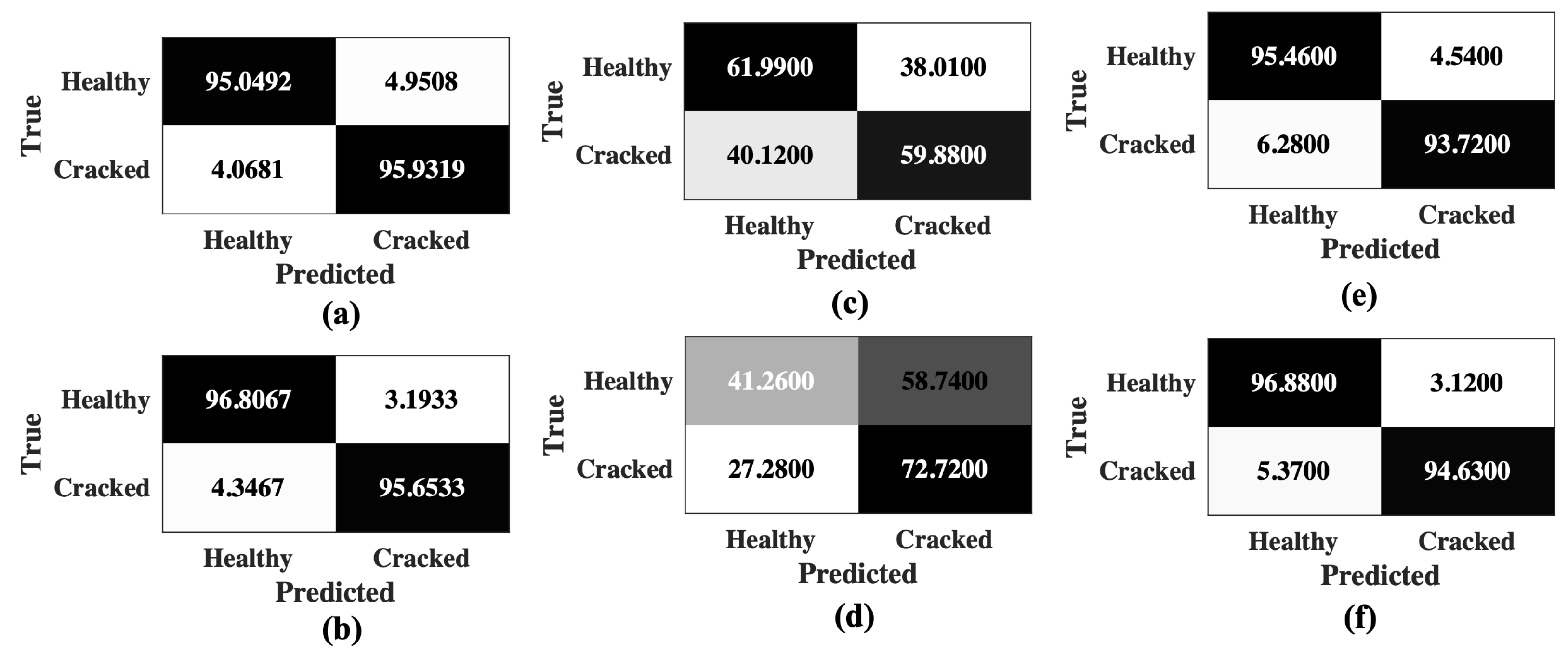
This paper presents a fatigue crack detection paradigm using ultrasonic signals through deep learning across different $K_t$s. Two baseline DNNs are trained for two different stress concentration factors ($K_{t1}$ and $K_{t2}$). An accuracy of 95.8% and 96.1% is observed, respectively, for $K_{t1}$ and $K_{t2}$. A transductive analysis is conducted to understand the capability of these pre-trained DNNs to detect damage in different $K_t$s. The analysis shows a steep drop in performance with accuracies of roughly 60%, indicating the disparity in the seemingly identical data from both the $K_t$s. To build a unified damage detection DNN, a mixed learning approach is developed by combining the data from both $K_t$s and training a single network. The mixed approach successfully demonstrates performance closer to the baseline DNNs. Delving further into the properties of mixed DNNs, a parametric analysis is conducted by varying the amount of training data used from each $K_t$. A gradual increase in performance is observed with an increase in the percentage of training data from 10% to 80% for both $K_t\mathrm{s}$. Incredibly, even with low training data, accuracies above 90% are observed in the analysis. The study, therefore, provides a basis for retraining with scarcely available data.

All DNNs in this analysis are developed in-house without using any of the existing pretrained networks. A study on fatigue-crack detection using a scattered-wave two-dimensional cross-correlation imaging method [38] shows an accuracy of 96% for the detection of 5-mm-long cracks and an accuracy of 99% for the detection of 10-mm-long cracks. However, the proposed method is able to detect cracks of the order of 3 micrometers of crack opening displacements with a maximum accuracy of 96% using relatively inexpensive ultrasonic sensors, thus showing that this method is not just feasible but actually superior to the existing techniques under certain scenarios. From a data analysis perspective, a common competitor to the mixed learning approach is transfer learning [35], which can also be used to solve a similar problem. A preceding study [27] with transfer learning shows similar accuracies to the mixed learning approach. However, mixed learning triumphs over transfer learning by eliminating the need for multiple DNNs. The combination of high accuracy, ease of deployment, and parametric retraining can, therefore, make DNNs a fantastic choice in fatigue-damage detection across industries.

However, the study does have some shortcomings that need to be addressed. The current approach investigates the question at hand as a binary classification problem without taking into consideration the sequence information present inside the time series. This is a reason why most of the erroneous predictions are around the area in the time series where the crack first appears. Such behavior is expected because there is very little visual or mathematical difference between the signals immediately before and after the short crack initiation. Incorporating sequence information within the models, using long short-term memory (LSTM) or generative adversarial network (GAN), might be able to boost our accuracy further. Moreover, DNNs serve very much as a ’black-box’ model: it is difficult to understand what features the model has learned in order to solve the problem of fatigue crack detection. Employing an encoder–decoder-based structure can allow the extraction of features from a 2D latent space. A systemic study of these features may allow us to gain a deeper understanding of the mechanics of fatigue failure and, thus, serve as an area of interest for future investigations.

References

1. Sofronas, A. Case Histories in Vibration Analysis and Metal Fatigue for the Practicing Engineer; John Wiley & Sons: Hoboken, NJ, USA, 2012. [Google Scholar]
2. Stephens, R.I.; Fatemi, A.; Stephens, R.R.; Fuchs, H.O. Metal Fatigue in Engineering; John Wiley & Sons: Hoboken, NJ, USA, 2000. [Google Scholar]
3. Suresh, S. Fatigue of Materials; Cambridge University Press: Cambridge, UK, 1998. [Google Scholar]
4. Besten, H.d. Fatigue damage criteria classification, modelling developments and trends for welded joints in marine structures. Ships Offshore Struct. 2018, 13, 787–808. [Google Scholar] [CrossRef]
5. Liao, D.; Zhu, S.P.; Correia, J.A.; De Jesus, A.M.; Berto, F. Recent advances on notch effects in metal fatigue: A review. Fatigue Fract. Eng. Mater. Struct. 2020, 43, 637–659. [Google Scholar] [CrossRef]
6. Yaghoobi, M.; Stopka, K.S.; Lakshmanan, A.; Sundararaghavan, V.; Allison, J.E.; McDowell, D.L. PRISMS-Fatigue computational framework for fatigue analysis in polycrystalline metals and alloys. NPJ Comput. Mater. 2021, 7, 1–12. [Google Scholar] [CrossRef]
7. Stopka, K.S.; Yaghoobi, M.; Allison, J.E.; McDowell, D.L. Effects of boundary conditions on microstructure-sensitive fatigue crystal plasticity analysis. Integr. Mater. Manuf. Innov. 2021, 10, 393–412. [Google Scholar] [CrossRef]
8. Pilkey, W.D.; Pilkey, D.F.; Bi, Z. Peterson’s Stress Concentration Factors; John Wiley & Sons: Hoboken, NJ, USA, 2020. [Google Scholar]
9. Liu, H.; Guo, S.; Chen, Y.F.; Tan, C.Y.; Zhang, L. Acoustic shearography for crack detection in metallic plates. Smart Mater. Struct. 2018, 27, 085018. [Google Scholar] [CrossRef]
10. Avci, O.; Abdeljaber, O.; Kiranyaz, S.; Hussein, M.; Gabbouj, M.; Inman, D.J. A review of vibration-based damage detection in civil structures: From traditional methods to Machine Learning and Deep Learning applications. Mech. Syst. Signal Process. 2021, 147, 107077. [Google Scholar] [CrossRef]
11. Farrar, C.R.; Lieven, N.A. Damage prognosis: The future of structural health monitoring. Philos. Trans. R. Soc. A Math. Phys. Eng. Sci. 2007, 365, 623–632. [Google Scholar] [CrossRef]
12. Yuan, F.G.; Zargar, S.A.; Chen, Q.; Wang, S. Machine learning for structural health monitoring: Challenges and opportunities. In Proceedings of the Sensors and Smart Structures Technologies for Civil, Mechanical, and Aerospace Systems 2020, Online, 27 April–9 May 2020; Volume 11379, p. 1137903. [Google Scholar]
13. Salehi, H.; Burgueño, R. Emerging artificial intelligence methods in structural engineering. Eng. Struct. 2018, 171, 170–189. [Google Scholar] [CrossRef]
14. Azimi, M.; Eslamlou, A.D.; Pekcan, G. Data-driven structural health monitoring and damage detection through deep learning: State-of-the-art review. Sensors 2020, 20, 2778. [Google Scholar] [CrossRef]
15. Zhao, R.; Yan, R.; Chen, Z.; Mao, K.; Wang, P.; Gao, R.X. Deep learning and its applications to machine health monitoring. Mech. Syst. Signal Process. 2019, 115, 213–237. [Google Scholar] [CrossRef]
16. Munawar, H.S.; Hammad, A.W.; Haddad, A.; Soares, C.A.P.; Waller, S.T. Image-Based Crack Detection Methods: A Review. Infrastructures 2021, 6, 115. [Google Scholar] [CrossRef]
17. Ebrahimkhanlou, A.; Salamone, S. Single-sensor acoustic emission source localization in plate-like structures using deep learning. Aerospace 2018, 5, 50. [Google Scholar] [CrossRef] [Green Version]
18. Mylonas, C.; Tsialiamanis, G.; Worden, K.; Chatzi, E.N. Bayesian graph neural networks for strain-based crack localization. In Data Science in Engineering, Volume 9; Springer: Berlin/Heidelberg, Germany, 2022; pp. 253–261. [Google Scholar]
19. Amiri, N.; Farrahi, G.; Kashyzadeh, K.R.; Chizari, M. Applications of ultrasonic testing and machine learning methods to predict the static & fatigue behavior of spot-welded joints. J. Manuf. Process. 2020, 52, 26–34. [Google Scholar]
20. Bansode, V.M.; Billore, M. Crack detection in a rotary shaft analytical and experimental analyses: A review. Mater. Today Proc. 2021, 47, 6301–6305. [Google Scholar] [CrossRef]
21. Dharmadhikari, S.; Basak, A. Fatigue damage detection of aerospace-grade aluminum alloys using feature-based and feature-less deep neural networks. Mach. Learn. Appl. 2022, 7, 100247. [Google Scholar] [CrossRef]
22. Xu, L.; Yuan, S.; Chen, J.; Ren, Y. Guided wave-convolutional neural network based fatigue crack diagnosis of aircraft structures. Sensors 2019, 19, 3567. [Google Scholar] [CrossRef] [Green Version]
23. Perfetto, D.; De Luca, A.; Perfetto, M.; Lamanna, G.; Caputo, F. Damage Detection in Flat Panels by Guided Waves Based Artificial Neural Network Trained through Finite Element Method. Materials 2021, 14, 7602. [Google Scholar] [CrossRef]
24. Califano, A.; Foti, P.; Berto, F.; Baiesi, M.; Bertolin, C. Predicting damage evolution in panel paintings with machine learning. Procedia Struct. Integr. 2022, 41, 145–157. [Google Scholar] [CrossRef]
25. Basak, A.; Das, S. Epitaxy and microstructure evolution in metal additive manufacturing. Annu. Rev. Mater. Res. 2016, 46, 125–149. [Google Scholar] [CrossRef]
26. Angel, N.M.; Basak, A. On the Fabrication of Metallic Single Crystal Turbine Blades with a Commentary on Repair via Additive Manufacturing. J. Manuf. Mater. Process. 2020, 4, 101. [Google Scholar] [CrossRef]
27. Dharmadhikari, S.; Raut, R.; Bhattacharya, C.; Ray, A.; Basak, A. Assessment of Transfer Learning Capabilities for Fatigue Damage Classification and Detection in Aluminum Specimens with Different Notch Geometries. Metals 2022, 12, 1849. [Google Scholar] [CrossRef]
28. Kannan, A.; Datta, A.; Sainath, T.N.; Weinstein, E.; Ramabhadran, B.; Wu, Y.; Bapna, A.; Chen, Z.; Lee, S. Large-scale multilingual speech recognition with a streaming end-to-end model. arXiv 2019, arXiv:1909.05330. [Google Scholar]
29. ASTM E466-15; Standard Practice for Conducting Force Controlled Constant Amplitude Axial Fatigue Tests of Metallic Materials. ASTM International: West Conshohocken, PA, USA, 2015.
30. ASTM B209; Standards Specification for Aluminum and Aluminum-Alloy Sheet and Plate. ASTM International: West Conshohocken, PA, USA, 1996.
31. Dharmadhikari, S.; Bhattacharya, C.; Ray, A.; Basak, A. A Data-Driven Framework for Early-Stage Fatigue Damage Detection in Aluminum Alloys Using Ultrasonic Sensors. Machines 2021, 9, 211. [Google Scholar] [CrossRef]
32. Dharmadhikari, S.; Basak, A. Energy dissipation metrics for data-driven fatigue damage detection in the short crack regime. In Proceedings of the ASME Turbo Expo, Virtual, 7–11 June 2021. [Google Scholar]
33. Dharmadhikari, S.; Basak, A. Evaluation of Early Fatigue Damage Detection in Additively Manufactured AlSi10Mg. In Proceedings of the 2021 International Solid Freeform Fabrication Symposium, Virtual, 2–4 August 2021. [Google Scholar]
34. Dharmadhikari, S.; Keller, E.; Ray, A.; Basak, A. A dual-imaging framework for multi-scale measurements of fatigue crack evolution in metallic materials. Int. J. Fatigue 2021, 142, 105922. [Google Scholar] [CrossRef]
35. Goodfellow, I.; Bengio, Y.; Courville, A.; Bengio, Y. Deep Learning; MIT Press: Cambridge, UK, 2016; Volume 1. [Google Scholar]
36. Géron, A. Hands-On Machine Learning with Scikit-Learn, Keras, and TensorFlow: Concepts, Tools, and Techniques to Build Intelligent Systems; O’Reilly Media: Sebastopol, CA, USA, 2019. [Google Scholar]
37. Bhattacharya, C.; Dharmadhikari, S.; Basak, A.; Ray, A. Early detection of fatigue crack damage in ductile materials: A projection-based probabilistic finite state automata approach. ASME Lett. Dyn. Syst. Control 2021, 1, 041003. [Google Scholar] [CrossRef]
38. Xiao, W.; Yu, L.; Joseph, R.; Giurgiutiu, V. Fatigue-Crack Detection and Monitoring through the Scattered-Wave Two-Dimensional Cross-Correlation Imaging Method Using Piezoelectric Transducers. Sensors 2020, 20, 3035. [Google Scholar] [CrossRef] [PubMed]
Figure 1. (a) A block diagram highlighting the impact of stress concentration on fatigue failure. A schematic of the (b) traditional machine learning and (c) proposed mixed learning model inspired by multilingual deep neural networks.
Applsci 13 01542 g001
Figure 2. Specimen designs for (a) K t 1 and (b) K t 2 (all dimensions are in mm).
Applsci 13 01542 g002
Figure 3. Local stress field visualization for (a) K t 1 and (b) K t 2 specimens using a finite element-based simulation.
Applsci 13 01542 g003
Figure 4. Comparison between the crack detection and failure instances for K t 1 and K t 2 in terms of the number of load cycles.
Applsci 13 01542 g004
Figure 5. (a) Custom fatigue testing apparatus highlighting the specimen, confocal microscope, moving stage, and grips. (b) Ultrasonic sensors mounted with a 3D-printed housing on the specimens. Reprinted from [27] with permission under the terms and conditions of the Creative Commons Attribution (CC BY) license.
Applsci 13 01542 g005
Figure 6. Concatenated Ultrasonic Signal for (a) K t 1 and (b) K t 2 . Three zoomed-in windows attributed as 1, 2, and 3 are shown in the corresponding insets.
Applsci 13 01542 g006
Figure 7. (a) A schematic showing the orientation of the confocal microscope. (b) A representative imaging of the region of high stress. (ce) Damage progression through a part of the high-stress region in the healthy, crack detection, and crack growth stages, respectively.
Applsci 13 01542 g007
Figure 8. ‘Healthy’ and ‘cracked’ labeling of the ultrasonic signals for (a) K t 1 and (b) K t 2 .
Applsci 13 01542 g008
Figure 9. (a) Using the healthy and cracked labels from the confocal microscope, an individual DNN can be trained and tested for either K t 1 or K t 2 using the respective dataset. (b) A single mixed DNN can be trained and tested from both K t 1 and K t 2 data.
Applsci 13 01542 g009
Figure 10. (a) Training and testing dataset bifurcation independently for K t 1 and K t 2 . (b) Baseline DNN training and testing with respective datasets for both K t s. (c) Baseline DNN architecture. (d) Transductive analysis—evaluating pre-trained DNNs in (b) by switching the test datasets for each K t .
Applsci 13 01542 g010
Figure 11. A single mixed DNN ( D N N T r a i n : 80 K t 1 + 80 K t 2 ) trained using a mixed dataset comprising of both K t 1 and K t 2 data; tested on data from both K t s separately.
Applsci 13 01542 g011
Figure 12. Confusion matrices for (a) K t 1 baseline DNN and (b) K t 2 baseline DNN. Confusion matrices for (c,d) transductive analysis, and (e,f) mixed learning. Reprinted (ad) from [27] with permission under the terms and conditions of the Creative Commons Attribution (CC BY) license.
Applsci 13 01542 g012
Figure 13. Distributions of the sensitivity, specificity, and accuracy of the K t 1 test data with variations in the training data percentages for (a) K t 1 and (b) K t 2 . The center lines in the boxplots represent the median, and the outliers are shown with diamonds.
Applsci 13 01542 g013
Figure 14. Distributions of the sensitivity, specificity, and accuracy of the K t 2 test data with variations in the training data percentages for (a) K t 1 and (b) K t 2 . The center lines on the boxplots represent the median, and the outliers are shown with diamonds.
Applsci 13 01542 g014
Figure 15. Contour plots showing variations in (a,b) Accuracy, (c,d) Sensitivity, and (e,f) Specificity for K t 1 and K t 2 , respectively.
Applsci 13 01542 g015