Comparative Analysis for Slope Stability by Using Machine Learning Methods

Featured Application

The presented paper conducted a comparative analysis based on well-known MLP, SVM, DT, and RF learning methods to assess/predict the safety factor (F.S) of earthslopes.

Abstract

Earth slopes’ stability analysis is a key task in geotechnical engineering that provides a detailed view of the slope conditions used to implement appropriate stabilizations. In the stability analysis process, calculating the safety factor (F.S) plays an essential part in the stability assessment, which guarantees operations’ success. Providing accurate and reliable F.S can be used to improve the stability analysis procedure as well as stabilizations. In this regard, researchers used computational intelligent methodologies to reach highly accurate F.S calculations. The presented study focused on the F.S estimation process and attempted to provide a comparative analysis based on computational intelligence and machine learning methods. In this regard, the well-known multilayer perceptron (MLP), decision tree (DT), support vector machines (SVM), and random forest (RF) learning algorithms were used to predict/calculate F.S for the earth slopes. These machine learning classifiers have a strong capability predict the F.S under certain conditions for slope failures and uncertainties. These models were implemented on a dataset containing 100 earth slopes’ stabilities, recorded based on F.S from various locations in the provinces of Fars, Isfahan, and Tehran in Iran, which were randomly divided into the training and testing datasets. These predictive models were validated by Janbu’s limit equilibrium analysis method (LEM) and GeoStudio commercial software. Regarding the study’s results, MLP (accuracy = 0.901/precision = 0.90) provides more accurate results to predict the F.S than other classifiers, with good agreement with LEM results. The SVM algorithm follows MLP (accuracy = 0.873/precision = 0.85). Regarding the estimated loss function, MLP obtained a 0.29 average loss in the F.S prediction process, which is the lowest rate. The SVM, DT, and RF obtained 0.41, 0.62, and 0.45 losses, respectively. This article tried to fill the gap in traditional analysis procedures based on advanced procedures in slope stability assessments.

1. Introduction

Slope stability is a crucial representation of rock, soil, or combined mass under various failures that lead to moving removable masses on a slope downstream [1]. Slope failures lead to ground deformation on a different scale and cause damage to facilities, roads, railways, infrastructures, and foundations [2,3]. The instabilities occurred under certain conditions or triggering factors, which can be related to the slope mass geometry, stress–strain history, geo-material status, external loadings, regional climate, seismic activity, pore water pressure conditions, and geo-structures. These triggering factors are used to determine the behavior of sliding mass and the potential slip surface expansion in slopes [4]. Slope mass geometry, or slope topography, can provide favorable conditions for slope mass sliding, falling, and overturning. In general, the likelihood of sliding rises as the slope angle gets steeper [2]. The presence of stress–strain history in a slope can cause ground movements, such as plastic slips and creep, which are mainly a time-dependent behavior of loose soils. Geo-material status is one of the well-known conditions that might provide a suitable condition for slope instabilities. The existence of loose layers or clay lenses, organic soils, marl, and glacial deposits are always considered essential drivers in slope failures [1]. External loadings and seismic activities can trigger the slope to failure under dynamic conditions, especially in an earthquake event, liquefaction, sand boils, dewatering of dams, tunnel boring, or heavy machinery. Regional climate responsibility for slow changes in slope conditions is known as weathering.

Weathering can be caused a decrease in the shear strength and durability of soil grains, which is considered a trigger for sliding in the slope [5,6]. Pore water pressure is one of the well-known motivating factors that leads slopes to failure. Most stability analysis equations consider the pore water pressure as one of the critical parameters in their calculations [1]. Pore water pressure is the pressure of groundwater held in soil (or rocks) at the pores between particles, increasing the fluidization of particles and reducing soil interparticle friction [4]. Finally, geo-structures are mostly related to faults, folding, and complex geological deformations that make ground changes. These structures provide appropriate conditions for particular failures such as debris, slope toe erosion, or side-base instabilities. Although many of these failures are related to rock slopes, numerous cases have also been observed in earth slopes [7,8].

In slope stability analysis, the slip surface that is considered as keyline between stable and unstable masses in a slope can be calculated based on the safety factor (F.S) index [1]. Regarding the geological composition of slopes, failures can be classified as earth slope and rock slope instabilities. Earth slopes act as homogeneous masses, which leads to the generation of the rotational (or massive failure) and planar forms. In rock slopes, the failure types are more varied, and the slope condition can be categorized as planar, wedge, toppling, and rotational failures [9,10]. Regardless of the type of failure that occurs in slopes, using the possible slippery mass condition can lead to the calculation of the F.S for the slope. F.S can be estimated by closing the polyhedral forces’ vectors or moments in an equilibrium state at the assumed sliding surface regarding dynamic and/or static conditions for two- and/or three-dimensional spaces [4].

$$\mathrm{F}.\mathrm{S}=\frac{{\displaystyle \sum \mathrm{Resistance} \mathrm{forces} \mathrm{or} \mathrm{moments}}}{{\displaystyle \sum \mathrm{Activation} \mathrm{forces} \mathrm{or} \mathrm{moments}}}$$

(1)

If all assumptions and requirements are met, and these polyhedral force vectors are closed, the slope mass must be in equilibrium, and the stability analysis must be reliable. The non-closure polyhedral vectors (forces and/or moments) are exemplified by the failure to satisfy several key requirements [9].

In earth slopes, in the absence of resistant surfaces or bedrock or layering with high strength, the sliding surface passes through locations with the lowest resistance, and F.S will be at its minimum. Thus, the slope will be stable if the F.S_min is over the critical state (F.S = 1). On the other hand, if the F.S_min value is less than the critical state, the slope is unstable. Accurate estimation of the F.S value can be used for stabilizations and provide reliable stability analysis for the slopes. Various stability analysis techniques have been developed over 300 years to calculate the F.S and identify the probable slip surface, the instability scale, and failure mechanism, which are categorized as routine evaluations, limit state criteria, planar failure, limit equilibrium, numeric, hybrid, high-order, and intelligent methods [10,11,12,13]. Each of these approaches has its benefits and limitations; some of them, such as limit equilibrium methods (LEMs), have been of more interest due to their simplicity in implementation, fewer assumptions, and the capability of generalization and inoculation with other methods. Varied types of LEMs were used in stability analysis with a historical background, but Fellenius [14] is one of the pioneers of stability analysis by engineering and computational methods. The Fellenius method is an established stability analysis based on the moment equilibrium around the failure circle center was applied on a circular slip surface, which is correct for rotational failures. Bishop [15] provides a vertical force equilibrium and moment equilibrium-based method to quantify rotational failures. Nonveiller [16] extended Bishop’s method for the more complicated condition of massive failures. Fredlund et al. [17] introduce a simplified methodology based on slicing a main movable mass on an earth slope, which is used to calculate the F.S in rotational failures with circular slip surfaces. Janbu and his colleagues [18,19] provide detailed LEMs-based methods for analyzing the stability conditions of earth slopes, which are capable of implementation in the general shape of slip surfaces. After these, researchers developing LEMs-based stability methods received considerable attention, which led to the introduction and application of various LEMs in stability analysis. Several of the well-known methods can be mentioned, such as the Swedish [20], USACE [21], Lowe–Karafiath [20], Sarma [22], Spencer [23], Morgenstern–Price [24], and Correia [25] methods. LEMs provide close results in calculating F.S, and the difference in the estimated values for F.S is generally about 6% [26]. Zhu et al. [27] stated that the LEM-based methods could be generalized for all types of methods, which can be applied to all kinds of slip surfaces for different failure mechanisms. The conventional LEMs methods perform the progressive instability analysis using iterative processes due to the limitations of the assumed surface for slip parameter evaluations. By advancing computer application in slope stability analysis, the LEM-based methods are significantly improved and capable of solving more complicated equations regarding F.S, which cover the traditional procedures in LEM analysis. Particularly, computational intelligent methods provide a highly accurate prediction about the slope condition, failure mechanism, and risk potential to slip [5,27,28,29,30].

Advanced technologies including artificial intelligence, especially machine learning, have provided significant help in the stability analysis of earth slopes regarding F.S estimation using predictive models. Predictive models attempt to forecast and evaluate the F.S according to the machine learning rate and specific accuracy. Machine learning algorithms attempt to build methods to understand the current circumstance of target data, learn, and operate to learn using training data. Machine learning uses different applications of various algorithms, which are classified as shallow, and deep learning techniques also attempt to make predictions or decisions [31]. The predictions’ accuracy directly depends on the learning rate of the algorithms, which can correspond to learning paradigms, such as supervised, unsupervised, or reinforcement learning [32]. No matter what type of learning is utilized in predictions, each algorithm can be analyzed for performance to understand its precision and accuracy [33].

The main ideas of using machine learning techniques to provide a safety factor or F.S for slopes can be classified based on several motivations: (i) F.S is a crucial value to the safety design, and an essential reliance of innovation and reliability against slope failure is directly related to this factor. Therefore, providing a reliable F.S with a low error rate and high precision is crucial. Traditional procedures are primarily based on simplified analyses and certain assumptions, which increase the error rate of calculations. (ii) In slope stability analysis, there are typically uncertainties in the evaluation process, which reduces the precision of calculations. Traditional methods usually do not have the possibility to cover such uncertainties. However, machine learning, with the amount of repetition in learning, can cover these uncertainties laterally and improve performance. (iii) The important point of reliance in machine learning analysis is the possibility of measuring the accuracy and performance of learning models during prediction processes, which can be estimated by the confusion matrix, error table, or loss function. There is no such capability in the usual stability analysis methods. Assessing the model’s accuracy can be very useful in decision-making and conducting optimal stabilization strategies. Therefore, in traditional methods, stabilization strategies are made based on experience.

Generally, machine learning techniques can effectively be used to develop robust predictive models for slope stability and to predict key parameters and stabilize behaviors in geotechnical engineering applications where uncertainty is inherent. Uncertainty considerations are the main deficiency in empirical and statistical assessments, leading to an increased error rate for stability analysis. The most significant uncertainties in estimating the slope safety coefficient (F.S) for various indicators include pore water pressure, geo-material characteristics, slope geometry, and slope strength properties [4]. Therefore, it is considered a priority to use approaches that can best cover the uncertainties or have a better ability and performance than these uncertainties. Machine learning procedures are strong tools to reach that goal.

The present study attempted to use several well-known machine learning algorithms to provide highly accurate predictive models to estimate the F.S for earth slopes. In this regard, the multilayer perceptron (MLP), decision tree (DT), support vector machines (SVM), and random forest (RF) learning algorithms were considered as the primary analysis core. These algorithms have features and advantages that have caused researchers to use them in different works, especially geotechnical analysis and domain stability. These benefits are summarized as follows:

They can handle both classification and regression on linear and non-linear data;

-

They use hyperplane, nodes, and neurons, which act like a decision boundary between different classes;

-

Options and choices are set out logically at the same time, and costs are considered as well as potential benefits, which leads to calculating the capabilities and errors;

-

There is the possibility of measuring the amount of error and the accuracy of calculations depending on the complexity level of the analysis;

-

There is a reduction of calculation time and the possibility of using it in all stages of evaluation and stabilization;

-

They provide a higher level of accuracy in predicting outcomes, which automatically reduces the error rate;

-

They are easy to understand and provide tangible results.

2. Analysis Methods Principles

Machine learning is a field of artificial intelligence study devoted to understanding and developing “learn” methods or techniques that use data to enhance performance on a particular set of tasks. To make predictions, classifications, or decisions without being explicitly programmed to do so, machine learning algorithms construct a predictive model from training data and test from testing data. These processes help in understanding the models regarding learning stages, which are presented as ‘learning rate’. By increasing the learning rate of the predictive model, it is expected that the accuracy will increase and the calculation error will decrease [33]. The model performance was controlled using a confusion matrix and loss functions, the main controlling criteria in machine learning-based evaluations. Optimization is also closely related to machine learning: many learning problems are formulated on a training set to minimize loss function [31].

The confusion matrix is liable to evaluate the performance of the predictive models, and the loss function represents the learning rate and the model’s capability to operate accordingly. In both the matrix and loss table, criteria are varied from 0 to 1, 0 being the lowest performance and 1 being the highest performance. Thus, the models that reach 1 or near it obtain reliable operation. On the other hand, reaching 0 represents unreliable modeling. The loss function provides information about mathematical optimization and seeks to minimize errors regarding the prediction and measured values. Therefore, there is a difference between estimated and valid values for a data instance [31]. The matrix has calculated precision, recall, f1-score, and accuracy elements, known as evaluation criteria.

3. Methods and Materials

3.1. Analysis Method

The stability analysis of the earth slopes, MLP, SVM, DT, and RF classifiers are utilized, which are considered benchmark algorithms in machine learning. MLP is a fully-connected feed-forward type of artificial neural network (ANN) classifier that refers to an ANN-based net consisting of multiple perceptron layers. MLP contains at least three layers of nodes as input, hidden, and output, which are supervised learning techniques [31]. MLP mainly uses fully connected activation functions such as sigmoids or rectifier linear units (ReLU) to join the nodes in different layers and supervise learning techniques. Learning in the perceptron net occurred by changing connection weights after data processing according to the error rate in the output as opposed to the expected result [34]. The SVM is a supervised model for data analysis for regression and classification objectives [35]. SVM is a prediction procedure built on statistical learning frameworks or the Vapnik–Chervonenkis theory [36]. SVM can effectively carry out a linear or non-linear classification by kernel tricks that implicitly translate their inputs into feature spaces with high dimensions [35]. An SVM constructs hyperplane(s) in a high- or infinite-dimensional space, which is utilized for prediction, classification, regression, and outlier detection [37]. A decision tree (DT) is a tool for decision support that uses a tree-like model of decisions and the potential outcomes of those decisions. An algorithm that only contains conditional control statements can be displayed in this manner. DT is frequently applied in operations, primarily in decision analysis, to assist in determining the most effective strategy for achieving a goal, but it is also a well-liked machine learning tool. DT is a flowchart-like structure whose internal nodes each represent a “test” on an attribute; the closely related influence diagram is used as a visual and analytical tool to help make decisions that can be linearized into decision rules [38]. Many decision trees are built during training to carry out the classification, regression, and prediction steps of the random forest (RF) algorithm, an ensemble-based learning technique [39].

Precision can be estimated as true positive/(true positive + false positive); recall is true positive/(true positive + false negative); accuracy is (true positive + true negative)/(true positive + true negative + false positive + false negative); and f1-score is 2 × (precision × recall)/(precision + recall). The coordination of the positivity and negativity of the variables is presented in Figure 1 [40]. The models learned under specific optimizing functions that improve the learning rates. The learning rate is a configurable hyperparameter utilized in the training procedures for machine learning algorithms.

Table 1. The hyperparameters used in the utilized models.

Classifier	Hyperparameters	Elements
MLP	Hidden layers’ size Learning rate Optimization	Activation = ’relu’; Optimization = rmsprop; Loss_function = ’mse’; Metrics = ’mae’
SVM	Kernels C value	Kernel =‘poly’; Degree = 2 C = 100; Epsilon = 0.1
DT	Max depth Random state	Criterion = ‘gini’; Max_depth = 5 Ccp_alpha = 0.0; Min_samples_leaf = 1 Random_state = 100
RF	Number of estimators Max depth	Criterion = ‘entropy’; N_estimators = 10; Max_depth = 5; Min_samples_leaf = 1; Min_sanmples_split = 2

provides information about the utilized hyperparameters in different applied classifiers.

3.2. Data Preparations

To utilize the benchmark learning algorithms that were carried out in the Python programming language, an extensive primary dataset was used. The main dataset contains 100 earth slope stability records based on F.S from various locations in Fars, Isfahan, and Tehran in Iran. The mentioned dataset was randomly divided into a training set (70% of the primary dataset) and a testing set (30% of the primary dataset). All predictive models were trained by the training set and validated with the testing set. The training set contains 70 slope stability records and the testing set contains 30 remaining slope data. The coefficient of Determination (R²) was used to establish correlations between the predicted and measured data during the evaluation steps.

3.3. Model Implementations

The first step in modeling is providing the primary dataset, which plays a key role in the prediction process. The main dataset provided actual data from the different earth slope investigations and was utilized in the preparation of testing and training sets. Models were trained with a training set and tested with a testing set regarding the accuracy, model performance, and capability, which were estimated by the confusion matrix and loss function.

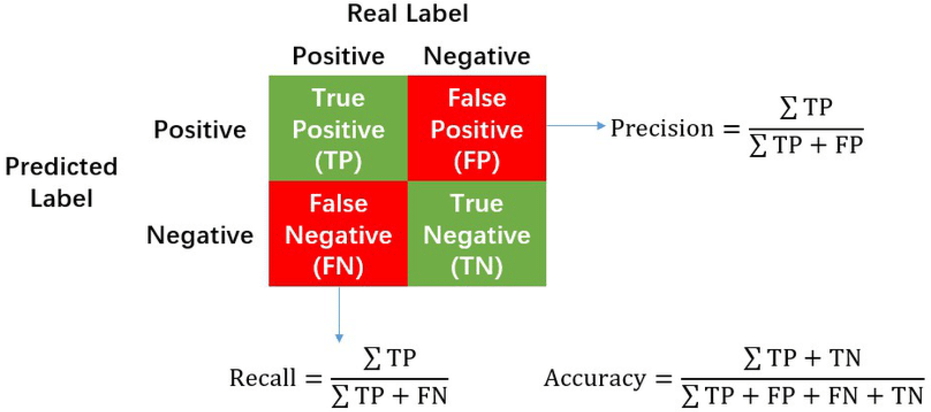
3.4. Models Validations

The ROC (receiver operating characteristic) curve is applied to validate the predictive models. ROC is a diagram made by plotting the true positive rate against the false positive rate, which represents an overall accuracy, and it shows the diagnostic capacity of a binary classifier system, as well as the range of its discrimination threshold. In this study, comparative verification was also provided by the ROC curve. On the other hand, it is necessary to provide the reliability of the estimated F.S the models, which were justified by limit equilibrium analysis methods (LEMs). The entire database was analyzed regarding slope stability by LEMs and GeoStudio commercial software. The results of the LEMs were used to trace the degree of reliability for predicted F.S by the machine learning methods.

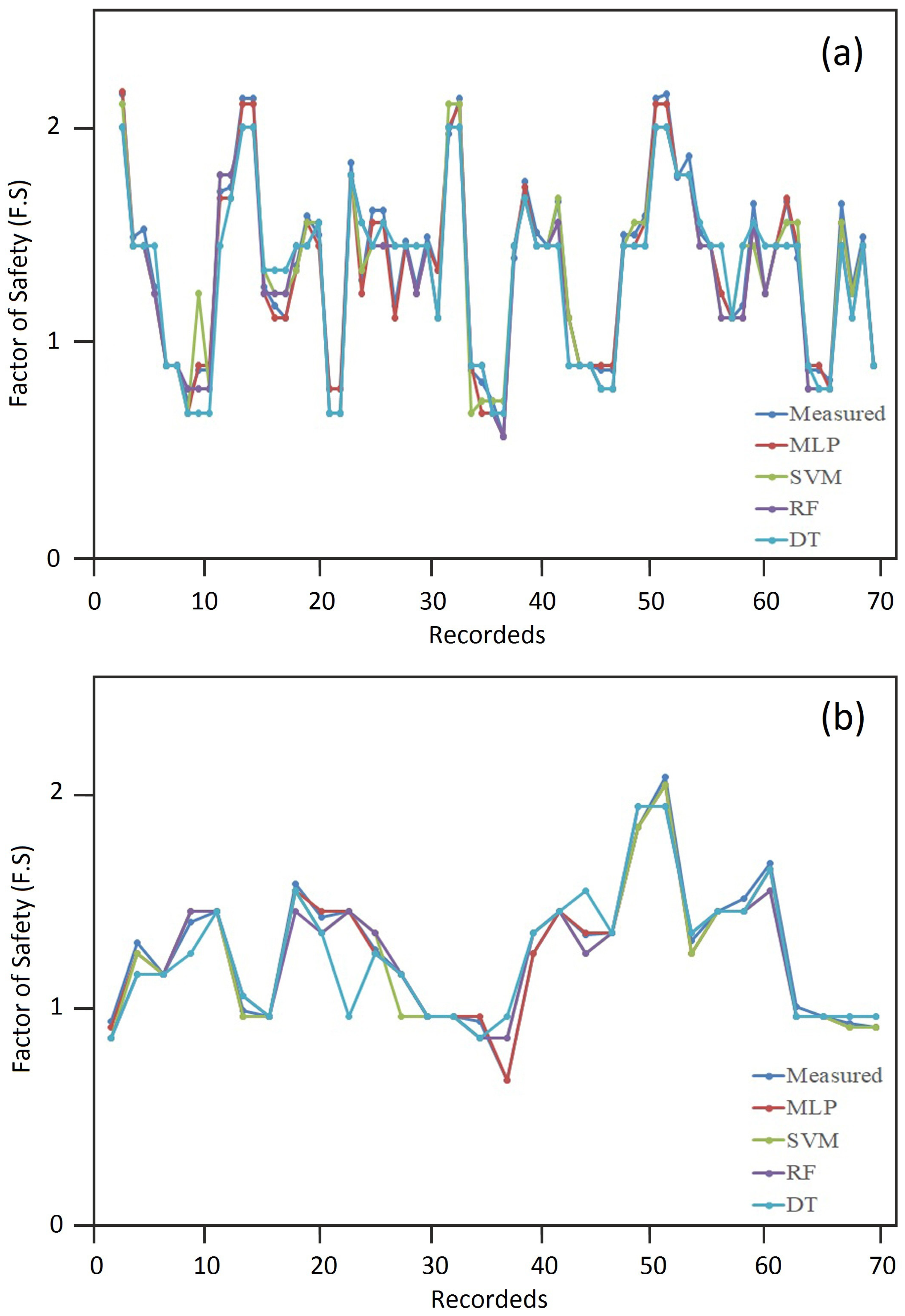
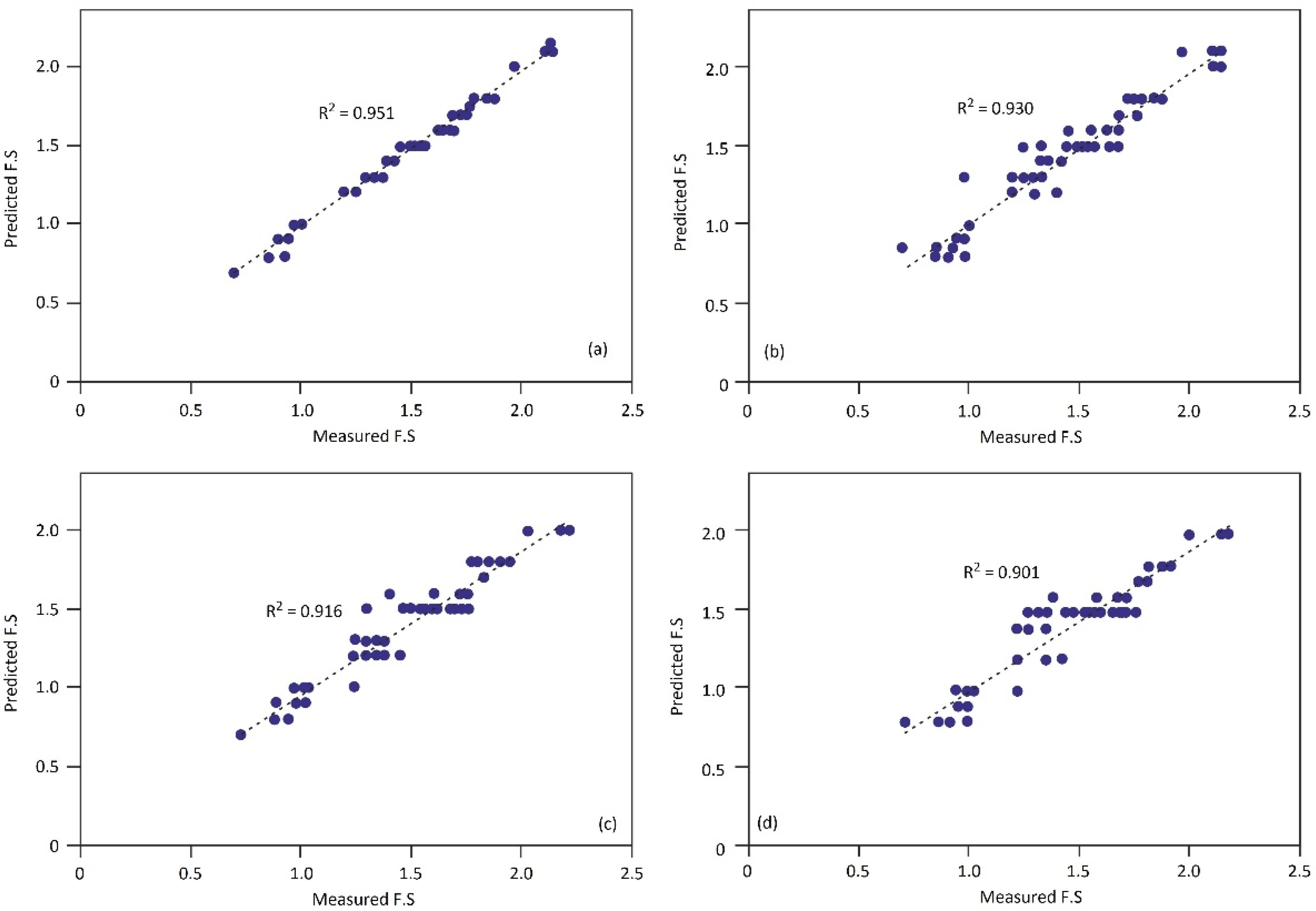
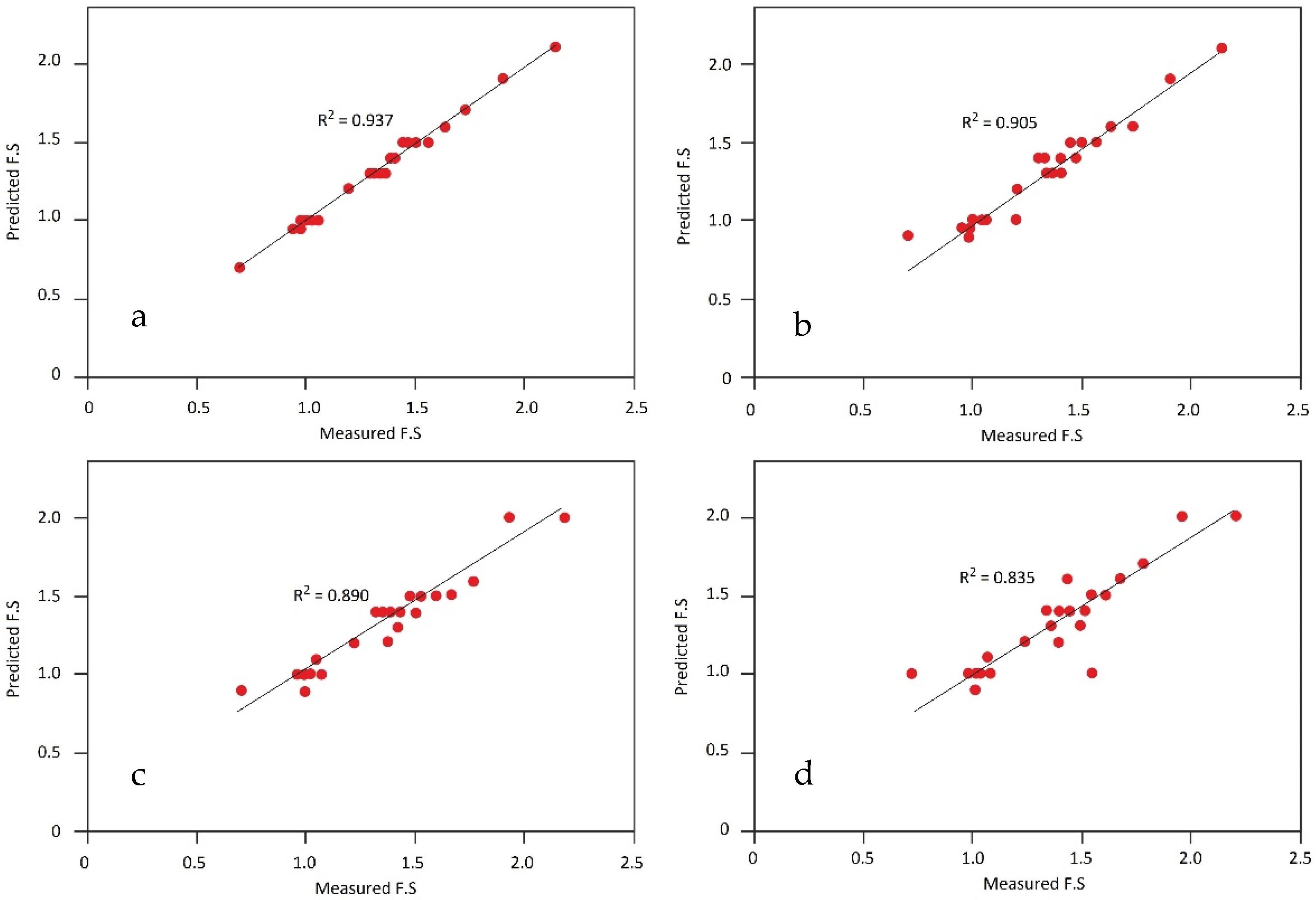
4. Results and Discussion

Slope stability analysis evaluates the stability condition of a slope undergoing movement. F.S is a crucial aspect of a numerical description of slope stability. Various methodologies are used to investigate slope stability conditions, which have a background of up to 300 years [6]. With the advancement of technology, these methods have become more complex and their accuracy has increased. Generally, all applied/introduced methods require several input data which are measured by geotechnical procedures and tests known as geotechnical characteristics of the slope, and output became F.S. using artificial intelligence (machine learning) approaches, which are one of the most recently developed techniques that have received remarkable attention from geo-engineers, due to their capability for accurate evaluations of stability and F.S. Typical machine learning methods are utilized in this article to process and predict the F.S for earth slopes.

The predictive models were implemented on actual data to construct the primary dataset. The dataset belongs to 100 stability analyses recorded from the Fars, Isfahan, and Tehran provinces in Iran. The slopes are mainly selected from the road cut projects concerned about stability condition and its effects on roads. Therefore, the study results are susceptible to stabilization methods that imply rectification of the situation. All slopes were investigated and the geotechnical properties of earth slopes were estimated during field surveys and laboratory experiments.

Table 2. Studied slopes’ geometrical properties.

Parameter	Unit	Max	Min	Mean	St.Dv.
Slope height (H)	m	25	5.5	15.25	9.75
Slope angle (β)	Degree	73	30	51.5	21.25
Slope topography *	-	Rough	Smooth	-	-
Water level in slope	m	3	0	1.5	1.5
Layers number	-	1	1	1	0
Tensile crack depth	m	1.75	0.12	0.935	0.815
Sliding surfaces depth **	m	27.4	1.3	14.35	13.05

* Slope topography is estimated by intuitive mean ** Sliding surface is estimated by GeoStudio.

and

Table 3. Studied slopes’ geotechnical properties.

Parameter	Unit	Max	Min	Mean	St.Dv.
Water content	%	37.2	5.44	21.32	22.457
Specific gravity (Gs)	-	2.63	2.60	2.61	0.0212
γd	kN/m3	19	17	18	1.4142
Slope height	m	25	12	18.5	9.1923
Slope angle	Degree	72	40	56	22.627
Cohesion (c)	kPa	185	93	139	63.053
Friction (φ)	Degree	35	32	33.5	2.1213
Poisson’s ratio (υ)	-	0.35	0.33	0.034	0.0141

provide information about the analyzed slopes’ geometrical and geotechnical properties.

To obtain the geotechnical characteristics of the earth slope mass, some specimens were taken and moved to the geotechnical laboratory. The index geotechnical tests, such as uniaxial compression strength, UCS [41], direct-shear [42], and physical properties [43], are directly used in the stability analysis of slopes. Physical properties of the soils can be categorized as water content, specific gravity, and density (γ_d), which has a standard procedure for estimation developed by the American Society for Testing and Materials (ASTM). The density (γ_d) is the fundamental physical properties used in stability assessment as well as soil strength parameters, which include cohesion (c), soil internal friction (φ), Poisson’s ratio (υ), and stiffness indexes. The stiffness indexes are the soil’s deformational modulus, such as young or elastic modulus (E), shear modulus (G), and bulk modulus (k). The stiffness parameters can be calculated by using empirical equations, which are presented as follows [1]:

G = E/2 (1 + v)

(2)

K = E/3 (1 − 2v)

(3)

The properties of the slope materials estimated by these tests used to investigate the general stability of the earth slope are based on computer-based calculations. The index geotechnical properties of the slope mass that are considered for calculation are presented in Table 3. These data were used for stability analysis in both machine learning-based and LEMs modeling as input data, which led to obtaining F.S as output. The information about the geotechnical properties of earth slopes builds the primary dataset used in predictions. The training set is utilized for training the models, and the test set is applied to validate the predictions. Measured and predicted values obtained from LEM and predictive models were correlated by the R² index. R² is the link between the actual outcomes and the prediction values that generally range from 0 to 1, where if the value is closer to 1, a higher accuracy of the data overlap appears. Figure 2 provides the prediction results of F.S by different machine learning classifiers on recorded samples in different earth slope training and testing sets. According to this figure, generally, predictive models have learned the process at an appropriate rate. In the meantime, the MLP classifier reaches more predictability for F.S estimation.

The results of the prediction process that led to evaluating the F.S were controlled by GeoStudio commercial software. GeoStudio is a two-dimensional, fully integrated software suite with LEM-based stability analysis and six finite element applications in various sub-models. Utilizing Janbu’s method, the SLOPE/W was used in this study to determine the F.S. Table 3 provides the geotechnical properties of the main slopes used in the stability analysis. The data from this table were entered into machine learning algorithms and the SLOPE/W program. SLOPE/W followed the several-stage modeling process, which can be categorized as geometric modeling, assignment of behavioral and materials characteristics, boundary conditions, and stability solutions. These steps are performed for the entire dataset (100 different slopes) and solved to calculate the minimum F.S of slopes. The calculated F.S was compared with the results of the machine learning predictive models. During geometric modeling, the geometry and topography of the slope, such as height, slope angle, layers, thickness of layers, slope surface conditions, and other (any) morphological complications, are designed and simulated. The studied earth slopes are composed of Quaternary alluvium, and no special layering or unique feature has been observed. Therefore, the main variables in geometric modeling are height and slope angle, which are illustrated in Table 2. Using this information helps to provide appropriate geometrical modeling for slopes. After preparing the slope geometry, the boundary conditions and behavioral model must be assigned to the model. The boundary conditions are easily defined in SLOPE/W. The Mohr–Coulomb (MC) failure criteria were selected as a behavioral model for stability analysis. The Mohr–Coulomb criteria, which represent the linear envelope obtained from a plot of the shear strength of a material versus the applied normal stress, are used to define the shear strength of soils at various effective stresses [44,45,46,47,48]. Table 3 is the index geo-materials properties used in modeling that are estimated based on ground survey and laboratory experiments assigned into the model as ‘material’ specifications. When the models are prepared, they are solved based on Janbu’s method for slope stability analysis, and results are reported as F.S for slopes.

Table 4. Studied slopes’ geometrical properties.

No.	Slope Location	Gs	γd (kN/m3)	H (m)	β (o)	c (kPa)	φ (o)	F.S
1	Tehran	2.62	18.22	12	45	124	35	1.65
2	Fars	2.63	18.71	10	60	117	33	1.57
3	Fars	2.60	18.20	7	63	93	33	0.98
4	Isfahan	2.60	18.20	15	52	117	35	1.54
5	Tehran	2.62	17.93	17	45	128	35	1.42
6	Fars	2.62	18.00	20	63	155	32	1.57
7	Fars	2.60	18.22	10	67	155	32	1.65
8	Tehran	2.60	18.70	15	40	142	33	1.25
9	Tehran	2.60	17.57	7	45	120	35	1.73
10	Isfahan	2.63	18.00	17	52	117	35	1.33

summarizes the ten studied slope stability calculations conducted by GeoStudio software as an illustration of the primary database used in predictive and LEM-based modeling.

Figure 3 and Figure 4 provide the results of the prediction process by the different classifiers plotted against measured data obtained from the LEM method via GeoStudio commercial software. The R² coefficients are estimated for both training and testing sets for all predictive algorithms with LEMs. According to these figures, MLP with R² = 0.951 in training and R² = 0.937 in testing stages reached the highest correlation with LEMs’ results. This shows that the MLP classifier can effectively and accurately evaluate the F.S coefficient for earth slopes and provides more reliable results. A look at other class clauses, such as SVM, shows that this classifier is in second place after the MLP method in the prediction of F.S. The SVM provides R² = 0.930 in training and R² = 0.905 in the testing process, which can be considered as near approximations of F.S values to actual data. DT and RF provide less correlation with the LEMs-based results.

A confusion matrix verified the entire predictive models and evaluation criteria (accuracy, precision, and recall), and the models’ loss rates were also estimated.

Table 5. The evaluation criteria estimate for predictive models.

Classifier	Dataset	Assessment Score			Accuracy
		Precision	Recall	F1-Score
MLP	Training	0.90	0.90	0.91	0.901
	Testing	0.91	0.85	0.91
SVM	Training	0.85	0.85	0.87	0.873
	Testing	0.85	0.87	0.87
DT	Training	0.81	0.83	0.83	0.812
	Testing	0.80	0.80	0.80
RF	Training	0.85	0.83	0.83	0.835
	Testing	0.83	0.83	0.85

and

Table 6. Estimated loss functions for used models.

Classifier	Maximum Loss	Minimum Loss	Mean Loss
MLP	0.4873650	0.1104769	0.298921
SVM	0.5798631	0.2546394	0.417251
DT	0.7506439	0.4934867	0.622065
RF	0.6007535	0.3010182	0.450886

provide information about the confusion matrix and loss function for different classifiers. Results of the confusion matrix approved the R² coefficient results, which show that the MLP operates with high accuracy (0.901) and precision (0.90). The SVM algorithm follows the MLP with accuracy (0.873) and precision (0.85). Regarding the estimated loss function results, it can be mentioned that MLP obtains a 0.29 average loss or cost in the prediction process, which is the lowest rate among the machine learning classifiers. The SVM, DT, and RF obtain 0.41, 0.62, and 0.45 losses, respectively. In Figure 5, the ROC curve analysis results of all models to evaluate the degree of the capability, which indicates that MLP provided the highest overall accuracy regarding the AUC (area under the curve) in the ROC curve, are illustrated. Based on the ROC curve results, MLP and SVM are reliable machine learning methods that can estimate F.S for earth slopes and provide suitable results. In the meantime, MLP can be recommended as an alternative technique that provides results that are appropriate and accurate. Referring to the ROC curve, MLP reaches an overall accuracy of up to AUC = 0.901 as the highest rank for the performance analysis of the machine learning classifier compared to the other classifiers. SVM and RF reach AUC = 0.873 and AUC = 0.835 as well. The lowest overall accuracy belongs to DT, with AUC = 0.812. In this regard, it is possible to say that the application of MLP can provide reliable and accurate results for F.S with good agreements with LEMs. Using such machine learning algorithms can help to develop an optimized method to understand the stability condition of earth slopes and suggest appropriate stabilization techniques to stabilize the slope. Other benefits of applying such techniques are reducing the cost of surveys, reducing calculation time, and increasing accuracy in complex stability analysis. Using these advantages helps geo-engineers to proceed with the stability analysis in the initial time of earthwork and the conduction of on-time stabilizations.

Compared to traditional methods, using machine learning techniques to develop an accurate prediction of F.S has a number of advantages and limitations. An advantage of the predictive models offered in this study is that they predicted a suitable and trustworthy estimate of F.S that could be applied to an analysis of the stability of an earth slope. Additionally, the comprehensibility and quickness of the achievements for prediction and classification have made it possible for users and personnel with low experience to use it well. Increases in the estimation’s accuracy for predicted outcomes can be presented by lowering error rates capable of being implemented in less time. An attitude towards the achievements of this research can state that the use of machine learning algorithms (mentioned classifiers) for predictions is independent of the sliding surface types and related to the input–output parameters for each stability class. Thus, it is possible to develop an extension method for other slope instabilities such as rock falls, shallow movements, debris, and toppling.

On the other hand, using machine learning algorithms has some limitations that should always be considered. The most important limit of machine learning algorithms is the database. A more extensive database is better and increases the learning rate. In geotechnical engineering, the input parameters are usually broad, with many uncertainties, so the development of highly accurate models must always have sufficient coverage in its database (both in the training and testing sets). The other limitation usually faced in the implementation process of predictive models is related to hardware and system analysis power. The higher system power is responsible for higher accuracy, higher complexity, and speed of analysis. Nevertheless, for future scientific research that might be conducted using machine learning applications by various researchers, it is recommended that scholars give specific attention to these limitations when they want to utilize machine learning methods.

5. Conclusions

The purpose of the presented study was to provide a comparative assessment of earth slope stability using benchmark learning classifiers. The objective of the study was to provide a more reliable and accurate procedure that can be used to estimate F.S for earth slope instability assessments. The MLP, SVM, DT, and RF algorithms were used to predict the F.S value as the primary variable or output of the models for the earth slopes. The primary database was prepared based on 100 records of earth slopes in Iran’s Fars, Isfahan, and Tehran provinces. The dataset contains records and geotechnical investigations of the slopes that were used in stability analysis. The main dataset was randomly divided into training and testing sets, which included 70% and 30% of the primary dataset. The classifiers were learned with a training set and validated with a testing set. Models were controlled by LEM-based stability analysis and measured F.S with GeoStudio software. For performance and capability analysis of the machine learning algorithms, confusion matrix, loss function, and ROC curves were utilized for all models and implemented in the Python programming language. As modeling results showed, MLP reached the highest accuracy (0.901) and precision (0.900). SVM and RF with accuracy = 0.873/precision = 0.850; and accuracy = 0.835/precision = 0.850 are ranked as the second and third algorithms that are properly used in F.S prediction. DT obtains the lowest accuracy in the confusion matrix, with accuracy = 0.812/precision = 0.810. The results were approved based on overall accuracy with ROC. The estimated losses for the models revealed that MLP is associated with the lowest loss rate (0.298921) and DT is associated with the highest loss rate (0.622065). This article tried to fill the gap in traditional analysis procedures based on advanced procedures in slope stability assessments.

References

1. Huang, Y.H. Slope Stability Analysis by the Limit Equilibrium Method; ASCE Publications: Reston, VA, USA, 2014. [Google Scholar]
2. Bromhead, E. The Stability of Slopes; Spon Press: New York, NY, USA, 1992. [Google Scholar]
3. Akgün, H.; Koçkar, M.K. Design of Anchorage and Assessment of the Stability of Openings in Silty, Sandy Limestone: A Case Study in Turkey. Int. J. Rock Mech. Min. Sci. 2004, 41, 37–49. [Google Scholar] [CrossRef]
4. Abramson, L.W.; Lee, T.S.; Sharma, S.; Boyce, G.M. Slope Stability Concepts: Slope Stabilization and Stabilization Methods, 2nd ed.; Wiley-Interscience: Millburn, NJ, USA, 2001. [Google Scholar]
5. Azarafza, M.; Hajialilue Bonab, M.; Derakhshani, R. A novel empirical classification method for weak rock slope stability analysis. Sci. Rep. 2022, 12, 14744. [Google Scholar] [PubMed]
6. Azarafza, M.; Akgün, H.; Ghazifard, A.; Asghari-Kaljahi, E.; Rahnamarad, J.; Derakhshani, R. Discontinuous rock slope stability analysis by limit equilibrium approaches–a review. Int. J. Digital Earth 2021, 14, 1918–1941. [Google Scholar] [CrossRef]
7. Bordoni, M.; Vivaldi, V.; Lucchelli, L.; Ciabatta, L.; Brocca, L.; Galve, J.P.; Meisina, C. Development of a data-driven model for spatial and temporal shallow landslide probability of occurrence at catchment scale. Landslides 2021, 18, 1209–1229. [Google Scholar]
8. Rotigliano, E.; Martinello, C.; Hernandéz, M.A.; Agnesi, V.; Conoscenti, C. Predicting the landslides triggered by the 2009 96E/Ida tropical storms in the Ilopango caldera area (El Salvador, CA): Optimizing MARS-based model building and validation strategies. Environ. Earth Sci. 2019, 78, 210. [Google Scholar] [CrossRef]
9. Kaur, A.; Sharma, R.K. Slope stability analysis techniques: A review. Int. J. Eng. Appl. Sci. Technol. 2016, 1, 52–57. [Google Scholar]
10. Albataineh, N. Slope Stability Analysis Using 2D and 3D Methods; University of Akron: Akron, OH, USA, 2006. [Google Scholar]
11. Azarafza, M.; Akgün, H.; Feizi-Derakhshi, M.-R.; Azarafza, M.; Rahnamarad, J.; Derakhshani, R. Discontinuous rock slope stability analysis under blocky structural sliding by fuzzy key-block analysis method. Heliyon 2020, 6, e03907. [Google Scholar]
12. Chen, Z.; Mi, H.; Zhang, F.; Wang, X. A Simplified Method for 3D Slope Stability Analysis. Canadian Geotech. J. 2003, 40, 675–683. [Google Scholar] [CrossRef]
13. Kliche, C.A. Rock Slope Stability, 2nd ed.; Society for Mining, Metallurgy, and Exploration Press: Englewood, NJ, USA, 2018. [Google Scholar]
14. Fellenius, W. Calculation of the Stability of Earth Dams. In Proceedings of the 2nd Transaction Congress on Large Dams (ICOLD), Washington, DC, USA, 1936. [Google Scholar]
15. Bishop, A.W. The use of Failure Circle in the Stability Analysis of Slopes. Geotechnique 1955, 5, 7–17. [Google Scholar] [CrossRef]
16. Nonveiller, E. The Stability Analysis of Slopes with a Slide Surface of General Shape. In Proceedings of the 6th International Conference on Soil Mechanics and Foundation Engineering, Montreal, QC, Canada, 8–15 September 1965. [Google Scholar]
17. Fredlund, D.D.; Krahn, J.; Pufahl, D.E. The relationship between limit equilibrium slope stability methods. In Proceedings of the International Conference on Soil Mechanics and Foundation Engineering, Stockholm, Sweden, 15–19 June 1981. [Google Scholar]
18. Janbu, N. Application of Composite Slip Surface for Stability Analysis. In Proceedings of the European Conference on Stability Analysis, Stockholm, Sweden, 1954. [Google Scholar]
19. Janbu, N.; Bjerrum, L.; Kjaernsli, B. Soil Mechanics Applied to Some Engineering Problems; Norwegian Geotechnical Institute Publication: Oslo, Norway, 1956. [Google Scholar]
20. US Army Corps of Engineers, USACE. Slope Stability: Engineering and Design; US Army Corps of Engineers Publications: Washington, DC, USA, 2003. [Google Scholar]
21. Lowe, J.; Karafiath, L. Stability of Earth Dams Upon Drawdown. In Proceedings of the 1st Pan American Conference on Soil Mechanic and Foundation Engineering, São Paulo, Mexico, 1960. [Google Scholar]
22. Sarma, S.K. Stability Analysis of Embankments and Slopes. Geotechnique 1973, 23, 423–433. [Google Scholar] [CrossRef]
23. Spencer, E. A Method of Analysis of the Stability of Embankments Assuming Parallel Inter-Slice Forces. Geotechnique 1967, 17, 11–26. [Google Scholar] [CrossRef]
24. Morgenstern, N.R.; Price, V.E. The Analysis of the Stability of General Slip Surfaces. Geotechnique 1965, 15, 79–93. [Google Scholar]
25. Correia, R.M. A limit equilibrium method of slope stability analysis. In Proceedings of the 5th International Symposium on Landslides, Lausanne, Switzerland, 10–15 July 1988. [Google Scholar]
26. Wyllie, D.C.; Duncan, C.; Mah, C. Rock Slope Engineerin, 4th ed.; Spon Press: London, UK, 2004. [Google Scholar]
27. Zhu, D.Y.; Lee, C.F.; Jiang, H.D. Generalized Framework of Limit Equilibrium Methods for Slope Stability Analysis. Geotechnique 2003, 53, 377–395. [Google Scholar] [CrossRef]
28. Ahangari Nanehkaran, Y.; Pusatli, T.; Chengyong, J.; Chen, J.; Cemiloglu, A.; Azarafza, M.; Derakhshani, R. Application of Machine Learning Techniques for the Estimation of the Safety Factor in Slope Stability Analysis. Water 2022, 14, 3743. [Google Scholar] [CrossRef]
29. Li, Y.X.; Yang, X.L. Soil-slope stability considering effect of soil-strength nonlinearity. Int. J. Geomech. 2019, 19, 04018201. [Google Scholar] [CrossRef]
30. Mathe, L.; Ferentinou, M. Rock slope stability analysis adopting Eurocode 7, a limit state design approach for an open pit. IOP Conf. Series: Earth Environ. Sci. 2021, 833, 012201. [Google Scholar]
31. Müller, A.C.; Guido, S. Introduction to Machine Learning with Python: A Guide for Data Scientists; O’Reilly Media: Sebastopol, CA, USA, 2016. [Google Scholar]
32. Aggarwal, C.C. Neural Networks and Deep Learning: A Textbook; Springer: Berlin/Heidelberg, Germany, 2018. [Google Scholar]
33. Azarafza, M.; Hajialilue Bonab, M.; Derakhshani, R. A Deep Learning Method for the Prediction of the Index Mechanical Properties and Strength Parameters of Marlstone. Materials 2022, 15, 6899. [Google Scholar] [CrossRef]
34. Vang-Mata, R. Multilayer Perceptrons: Theory and Applications; Nova Publications: Hauppauge, NY, USA, 2020. [Google Scholar]
35. Awad, M.; Khanna, R. Support vector regression. In Efficient Learning Machines; Apress: New York, NY, USA, 2015. [Google Scholar]
36. Cortes, C.; Vapnik, V.N. Support-vector networks. Machine Learning 1995, 20, 273–297. [Google Scholar] [CrossRef]
37. Cristianini, N.; Shawe-Taylor, J. An Introduction to Support Vector Machines and Other Kernel-based Learning Methods; Cambridge University Press: Cambridge, UK, 2000. [Google Scholar]
38. Sheppard, C. Tree-Based Machine Learning Algorithms: Decision Trees, Random Forests, and Boosting; Createspace Independent Publishing: Scotts Valley, CA, USA, 2017. [Google Scholar]
39. Pavlov, Y.L. Random Forests; De Gruyter Press: Berlin, Germany, 2018. [Google Scholar]
40. Ma, J.; Ding, Y.; Cheng, J.C.; Tan, Y.; Gan, V.J.; Zhang, J. Analyzing the leading causes of traffic fatalities using XGBoost and grid-based analysis: A city management perspective. IEEE Access 2019, 7, 148059–148072. [Google Scholar] [CrossRef]
41. ASTM D2166; Standard Test Method for Unconfined Compressive Strength of Cohesive Soil. ASTM International: West Conshohocken, PA, USA, 2006.
42. ASTM D3080; Standard Test Method for Direct Shear Test of Soils under Consolidated Drained Conditions. ASTM International: West Conshohocken, PA, USA, 2004.
43. ASTM C830; Standard Test Methods for Apparent Porosity, Liquid Absorption, Apparent Specific Gravity, and Bulk Density of Refractory Shapes by Vacuum Pressure. ASTM International: West Conshohocken, PA, USA, 2016.
44. Labuz, J.F.; Zang, A. Mohr–Coulomb failure criterion. Rock Mech. Rock Eng. 2012, 45, 975–979. [Google Scholar]
45. Yang, X.L.; Yin, J.H. Slope stability analysis with non-linear failure criterion. J. Eng. Mech. 2004, 130, 267–273. [Google Scholar]
46. Barvor, Y.J.; Bacha, S.; Qingxiang, C.; Zhao, C.S.; Siddique, M. Surface mines composite slope deformation mechanisms and stress distribution. Min. Mineral Dep. 2020, 14, 1–16. [Google Scholar] [CrossRef]
47. Sedina, S.; Altayeva, A.; Shamganova, L.; Abdykarimova, G. Rock mass management to ensure safe deposit development based on comprehensive research within the framework of the geomechanical model development. Min. Mineral Dep. 2022, 16, 103–109. [Google Scholar] [CrossRef]
48. Barvor, Y.J.; Bacha, S.; Qingxiang, C.; Zhao, C.S.; Mohammad, N.; Jiskani, I.M.; Khan, N.M. Research on the coupling effect of the composite slope geometrical parameters. Min. Mineral Dep. 2021, 15, 35–46. [Google Scholar] [CrossRef]
Figure 1. Basic information about the confusion matrix and evaluation criteria [40].
Applsci 13 01555 g001
Figure 2. Measured and predicted results’ correlation on different classifiers based on (a) training and (b) testing sets.
Applsci 13 01555 g002
Figure 3. Measured and predicted correlation for training results: (a) MLP, (b) SVM, (c) DT, (d) RF.
Applsci 13 01555 g003
Figure 4. Measured and predicted correlation for testing results: (a) MLP, (b) SVM, (c) DT, (d) RF.
Applsci 13 01555 g004
Figure 5. ROC curve analysis for different machine learning approaches.
Applsci 13 01555 g005