Abstract
Images taken with different sensors and transmitted through different channels can be noisy. In such conditions, the image most often suffers from random-valued impulse noise. Denoising an image is an important part of image preprocessing before recognition by a neural network. The accuracy of image recognition by a neural network directly depends on the intensity of image noise. This paper presents a three-stage image cleaning and recognition system, which includes a developed detector of pulsed noisy pixels, a filter for cleaning found noisy pixels based on an adaptive median, and a neural network program for recognizing cleaned images. It was noted that at low noise intensities, cleaning is practically not required, but noise with an intensity of more than 10% can seriously damage the image and reduce recognition accuracy. As a training base for noise, cleaning, and recognition, the CIFAR10 digital image database was used, consisting of 60,000 images belonging to 10 classes. The results show that the proposed neural network recognition system for images affected by to random-valued impulse noise effectively finds and corrects damaged pixels. This helped to increase the accuracy of image recognition compared to existing methods for cleaning random-valued impulse noise.
1. Introduction
Currently, solutions to the problem of pattern recognition are used in many applied and theoretical areas of modern science. Based on this, intensive research is being carried out on the creation of artificial intelligence systems in order to develop mathematical and software tools for modeling human thinking processes for the automatic solution of various applied and theoretical concerns. Applications of neural networks for solving such problems are security systems [1], educational [2] and advertising systems [3], art [4], gardening [5], image restoration [6], face recognition systems [7], etc.
However, it is impossible to use conventional methods with strict algorithms and limitations to solve recognition problems. Recognition issues do not have an algorithmic solution, so the initial data may be incomplete or erroneous. Also, the data used in recognition is often large, at a time when a person needs to set parameters and supplement information about an object. An automatic system that solves such problems should not be programmed but trained. For this reason, neural networks are one of the most promising tools for solving pattern recognition difficulties [8].
1.1. Related Works
Among all artificial intelligence technologies, convolutional neural networks (CNNs) are the most workable technology for pattern recognition, since such a ratio of hardware costs and the resulting accuracy is recognized as the most effective [9]. Among the main areas of application of neural networks are forecasting, decision-making, pattern recognition, optimization, and data analysis. Neural networks underlie most modern speech recognition and synthesis systems, as well as image recognition and processing. In [10], a modular model for predicting the level of tides was proposed, which could predict the level of tides by analyzing not only the movements of celestial bodies but also environmental factors. The work [11] is devoted to improving the accuracy of predicting metro traffic flows using a neural network with three recurrent blocks and a long short-term memory (LSTM) network. Convolutional networks have gained great popularity in the field of medical diagnostics. The authors of [12] used CNN and LSTM for natural language processing to extract features from an mRNA sequence to predict the miRNA sequence. The work [13] presented an improved cancer segmentation and detection method based on a generalized loss function with functional parameters determined adaptively during model training, to provide a universal basis for optimal decision-making based on a neural network. The problem of decision support under conditions of uncertainty can be solved using a fuzzy set model based on a backpropagation neural network [14]. In [15], a self-organizing computing network was presented based on the concepts of fuzzy conditions, beliefs, probabilities, and neural networks. It was presented in order to make decisions in intelligent systems that are necessary to process data sets with various types of data. The task of recognition and classification is one of the main tasks that neural networks solve. Recently developed capsule networks have already been used successfully for text recognition tasks [16]. Also, neural networks have been successfully applied to solve global optimization problems [17]. However, despite the scope of the neural network, the main task that is solved in all the above works is the task of increasing the recognition accuracy of given objects.
On the other hand, when creating, transmitting, and processing images, various noises arise [18], such as Gaussian, salt-pepper, Poisson, impulse, speckle noise, etc. Noise distorts image pixels. It is a destructive factor when training neural networks and it complicates the recognition and classification of objects not only for computer vision systems but also for the human eye [19]. Various types of noise, such as impulse noise, missing image samples, image packet loss, corrupted images, and distorted images, affect image quality and render images unsuitable for processing. For this reason, there is a search for a development of methods and for algorithms to solve the problems of cleaning digital images from various kinds of noise.
It should be noted that one of the most common types of noise that occurs when receiving, transmitting, and recording images is impulse noise. Impulse noise is explained by the fact that the intensity of the damaged pixel differs from the intensity of its neighbors [20]. In [21], for the task of removing impulse noise, the authors used non-linear filters; for example, an ascending M-estimator was introduced in the modified nearest neighbor filter. Work [22] is devoted to the use of a median filter, which replaces the value of the brightness of a distorted pixel with the average of its neighbors. Adaptive median filtering first determines if a pixel is skewed and then changes its value to avoid blurry objects [23]. The research [24] offers a convolutional neural network that can recognize noisy images without pre-processing by adding a noise map layer and an adaptive resizing layer, and by improving the overall noise resilience of the CNN. In recent years, scientists and researchers have often engaged in the development of various filters for cleaning random-valued impulse noise. The research [25] aimed to clean the image from impulse and Gaussian noise, using a method that was presented as a refinement of the bilateral filter for determining distorted pixels [26]. In [27], a method is described as an improvement to the method of [25] using a logarithmic function and threshold transformations. The authors of [28] also described a comparison of methods [25,27] and proposed a method that is another modification of the method [25]. The method introduced a new statistic of the Local Consensus Index (LCI), which is calculated by summing all pixel similarity values in its vicinity and finding the value of the central element. In [29], an algorithm was developed for detecting and cleaning random-valued impulse noise using the Gaussian probability distribution function and a median filter. The research [30] submits a two-stage denoising algorithm based on local pixel similarity and the subsequent purification of pulses by an improved bilateral filter. The work of [31] is similar to previous works in that it applied a two-stage denoising method—LCI and edge pixel detectors and an LCI-based filter were used. Some scientists have been able to apply fuzzy logic methods to effectively remove up to 50% of impulse noise from any image [32]. Our previous work is devoted to the use of a combination of a median and bilateral filter, which effectively removes high-intensity impulse noise [33].
1.2. Research Motivation
Thus, it is very important to completely clean up noisy images with a high noise density at the pre-processing stage [19]. However, this is not always possible, and the pre-processing for image restoration itself is an expensive and time-consuming process, which leads to low efficiency of training and validation of the neural network [24]. One of the ways to eliminate distortions is to use mathematical (and computer) processing of measurement results in order to eliminate distorting factors, and increase the resolution of instruments and the quality of image visualization. After obtaining a clearer image, the accuracy of identification (classification, recognition, diagnostics) of the object increases. Researchers [18] were among the first to implement Principal Component Analysis for filter generation in a convolutional neural network, which helped combine the neural network’s image classification capabilities with PCA’s reduction in computational overhead. In their research [19], Zheng et al. proposed to use a two-channel convolutional neural network model containing additional image features with enhanced contours. Thus, using the original and enhanced image, the accuracy of the dataset did not decrease. Some researches proved that training a neural network on mixed data (noisy and clean images) increases its resistance to these noises and improves classification accuracy [34]. To do this, special resizing layers must be used, as well as an adaptive union operator, to reduce noise interference [24]. For noise reduction reconstructed using positron emission tomography, a convolutional neural network can also be used. The classification of reconstructed images, compared to conventional noise smoothing, showed better results [35]. The DeQCANet quaternion convolutional neural network can remove color random-valued impulse noise using a new scheme for constructing a quaternion map and obtaining color characteristics by channels [36]. Jang et al. showed in their work that DNNs are susceptible to spatially uncorrelated white noise, and by introducing a noise learning procedure, it is possible to provide a better qualitative match to human performance [37]. In [38], a controlled random quantum neural network was proposed that used hybrid classical quantum algorithms with superposition and amplitude state coding functions, which improved not only the classification accuracy on MNIST, FashionMNIST, and KMNIST data, but also stability under conditions of increased noise. Also, a complex valued multilayer neural network with multivalued neurons (MLMVN) was adapted and successfully applied to filter impulse noise [39]. Despite a fairly large knowledge base and ongoing research in the field of image recognition using neural networks, none of the works offer a complex of a preprocessing filter and a recognizer. The pre-processing stage is necessary for a more accurate recognition result that is not spoiled by noise and impulses.
In general, the researchers either recognized noisy images or cleaned the image of impulse or other noise. There were no works that would combine the search and elimination of noisy pixels and their further recognition. We have combined these important steps and created a system that denoises images efficiently and recognizes pre-processed images with high accuracy. In this paper, we propose a neural network complex for recognizing images exposed to random-valued impulse noise. The presented system for the recognition of noisy images consists of a preprocessing stage, which includes a detector of distorted pixels, a system for their cleaning, and a neural network complex for recognizing cleaned images. The proposed method, in comparison with the existing ones, allows obtaining a gain in the accuracy of image recognition, which is confirmed by the experimental results of recognition of the same image, cleared of noise by different methods.
2. Methods
A neural network is a sequence of neurons connected by synapse connections. Neural network systems are mainly used for three tasks: classification, prediction, and pattern recognition [40]. In this case, the image is a complete or partial reflection of the properties of the object, while the result of recognition is the assignment of these initial data to a certain class, which means the establishment of the subject.
An important indicator of the accuracy of the neural network is the error. The error is the percentage of discrepancy between the expected and actual results of calculations [41]. Most often, MSE is used to maintain balance in the error calculation:
where —is an expected network response, —is an actual answer, and —is the number of training sets.
The Convolutional Neural Network (CNN) showed its best results in the field of recognition. Unlike a multilayer perceptron, this type of network takes into account the two-dimensional topology of the image and provides invariance to scaling, rotation, shifts, and spatial distortions [42]. The structure of the network is based on the implementation of a mathematical operation for extracting a feature map (convolution). If there are multiple convolutions in a layer Υ, each operation has an output dimension:
where —input image dimension, —the number of convolutions in the layer, and —is kernel size. Convolution kernels can be three-dimensional, in which case the dimension convolution is used on the first layer, and the output will be one image instead of three. Thus, the convolution operation reduces the image, while the outer pixels participate in fewer convolutions, which causes the need to complement the image at the edges. When applying the shift parameter, the output μ will look like:
When transmitting an image, various errors such as noise or loss of quality may occur. Most often, under these conditions, the image suffers from impulse noise. Impulse noise is characterized by the replacement of a part of the pixels in the image with the values of a fixed or random variable. Impulse noise is divided into fixed (“salt and pepper”) and random-valued [43]. In the second type of impulse noise, the distortions and their location are random and uniformly distributed in brightness and spatial arrangement. In an image noisy with random-valued impulse noise, the brightness value of some pixels is replaced by a random one [44]. Mathematically, this noise is described as:
where —image pixel, —original image, —noise value in the range [0,255].
Median filtering is used to eliminate impulse noise. This non-linear filtering handles the non-Gaussian distribution of real noise better than linear filters. When the differences in signal values are large compared to the variance of the Gaussian noise, the median filter gives a smaller value of the RMS error of the output signal with respect to the input, i.e., the non-noisy signal, with comparison to optimal linear filters. It is a window that sequentially slides over an array of image pixels and, at each step, returns one of the elements that fell into the aperture. The output signal of the moving median filter of width n for the current sample k is formed from the input time series in accordance with the formula:
where —elements of the variation series.
The width of the median filter is chosen, taking into account that it is able to suppress a pulse of width samples, provided that is an odd number. For each position of the window, the samples selected in it are ranked in ascending or descending order of values, and the sample average in its position in the ranked list is called the median if the number of samples is odd. This sample replaces the central sample in the window for the processed signal. For an even number of samples, the median is set as the arithmetic mean of the two average samples. Due to their characteristics, median filters with an optimally selected aperture can preserve sharp object edges without distortion, suppressing uncorrelated and weakly correlated noise and small-sized details.
3. Proposed Method and Results
3.1. Proposed Method
The paper proposes a neural network system for recognizing images exposed to random-valued impulse noise; the system has been built taking into account the stage of preliminary processing of incoming images for recognition by the system. Figure 1 shows the scheme of the proposed neural network system. The input was a color or grayscale image and entered the distorted pixel detector. Each pixel was examined for the presence of a pulse. Information about the location of noisy pixels in the form of a noise map G entered the cleaning system based on an adaptive median filter. A 3 × 3 window was used, but if all the pixels in this small window were noisy, then the filter was applied iteratively. After calculating the median of the neighbors of the distorted pixel, this value was assigned to it. Furthermore, the already cleaned image entered the neural network recognizer, and the result is displayed as a percentage between 10 categories, since the network was trained and tested on the basis of CIFAR10.
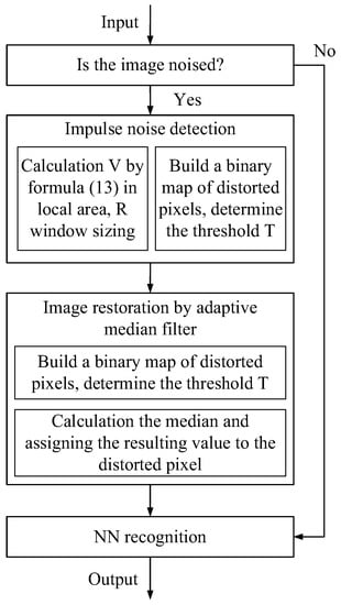
Figure 1.
Scheme of a neural network system for recognizing images exposed to random-valued impulse noise.
Recognizing and cleaning up random-valued impulse noise was a more difficult task than removing salt and pepper noise. A distinctive feature of the proposed scheme is the presence of a detector. The distorted pixel detector was specially designed and tested on various noise efficiencies and showed high cleaning results.
The developed detector, which is part of the image recognition neural network complex, is a 3 × 3 filter, which, by comparing the brightness of the central pixel and the brightness of its neighbors, revealed whether the pixel is noisy. The original brightness values may be close to the pulse values, and the distorted pixels may be nearby. The detection depends on the Euclidean distance between pixels and their brightness difference and calculates a weighted average value over a certain neighborhood. The similarity between any two pixels can be set as follows [45]:
where —coefficient of influence of the geometric distance between pixels, —coefficient of influence of brightness difference between pixels, and denote the pixel coordinates in the local area Ω, and —parameters of standard deviation of coefficients. The sum θ is calculated as follows:
Assuming that T is a threshold value selected empirically, and the array —map of noisy pixels, then from (8):
Thus, the value obtained from (8) is compared with the threshold T.
In known approaches, the threshold is usually selected experimentally, based on an empirical analysis of the results of the detector operation. In the proposed method, we will apply a similar approach for this purpose. We recommend choosing a threshold according to Table 1. It can be concluded that as the noise intensity in the image increases, the threshold value T decreases.

Table 1.
Threshold value T chosen for noise intensities N.
The proposed method used the distance between pixels and the difference in brightness values in the local window to determine the similarity between pixels. First, the pixel in question must be defined as noisy or clean. An estimate of the difference in the distance between pixels in the local window was calculated using (5). The figure represents the squared distances according to the Euclidean metric between the central pixel and its neighbors located in the window. The set of pixels, the coordinates of which are removed from the central pixel by a distance not greater than the specified R, represent the local window Ω of the detector. The distance between pixels and in the metric is determined according to:
In Figure 2, for a local window Ω with a radius of 4, the distance between the central and selected pixels is .
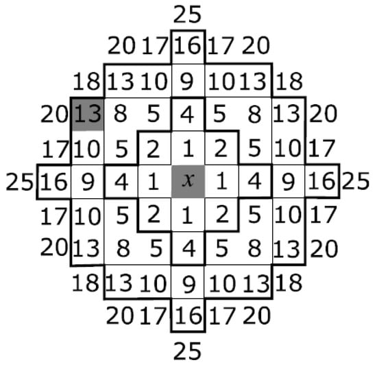
Figure 2.
The distance squared between the central pixel x and its neighbors. Lines mark local windows Ω with different radii.
For the convenience of visual perception of the result of cleaning the image from noise, the Euclidean metric was used. The metric is sufficiently suitable for calculating filter masks for cleaning images from impulse noise using adaptive median filtering [46]. When using pixel values from the previous and next frames, it was possible to create a mask to clean video data from random-valued impulse noise using the same metric [47].
The function of the absolute difference between the processed pixel and other pixels in the local window Ω is used to estimate the difference in brightness values between pixels:
where —is the bit depth of the image pixels. The smaller the value of is, the greater the brightness difference. Dividing by keeps non-negative. The logarithmic function indicates the most significant bit of the difference between pixels and is well suited to explain the digital nature of the data and to align with the visual perception of the human eye [48].
The second step is to sort the array in ascending order and sum the first elements of the sorted array, where is the number of elements in the local window Ω:
The similarity score between pixels W is calculated from (5) and (12):
To determine the presence of pixel distortion, a threshold is introduced:
If the array is a map of noisy pixels and if an element in is 1, the corresponding pixel in the image is noisy. The size of the local window Ω depends on the noise level. Experiments carried out within the framework of the proposed work showed that the direct relationship between the intensity of impulse noise and the size of the mask for its purification is the most effective.
For the recognition task, a neural network with a pretrained VGG16 architecture was used [49]. The 16-layer model, pretrained on the ImageNet data set, showed high results in the recognition accuracy of the CIFAR10 base, which is inferior to ImageNet in the amount of training data, that is 60,000 images versus 14,000,000 images. The model is an improved version of the first convolutional network AlexNet [50], in which large filters (sizes 11 and 5 in the first and second convolutional layers, respectively) are replaced by several filters of size 3 × 3, one after the other. Despite significant drawbacks, such as the heavy weight of the architecture and the low learning rate, the network is easily implemented and surpasses many other models in accuracy.
Let us present the results of the experiment of the influence of image cleaning methods from random-valued impulse noise on the accuracy of recognition of objects in the image by a neural network.
3.2. Experiment
Each RGB channel of the noise-exposed image was denoised separately from the other two at a fixed intensity 1%, 10%, 25%, or 50%. The 1, 10, 25, and 50 percent mean that the number of pixels in each image were randomly distributed. The experiment included recognition using a pretrained network of both individual noisy and clean images, and the entire test database. Table 2 shows the accuracies of pretrained architects to justify the choice of the basis of the image recognition program. A total of 20 epochs of each architectural network was trained and the highest value was chosen. The table shows that the best learning outcome was the VGG16 architecture. For 13 training epochs, the network recognized 8799 out of 10,000 test images, and thus the network reached a maximum accuracy of 87.99%, and the error at this epoch was 0.5190 (Figure 3). The learning rate was chosen as 0.01, the training batch had 64 images, and the test batch had 1000 images. The convolution filter 3 × 3 was used.
Table 2.
Best learning outcomes for architectures on CIFAR10 database.
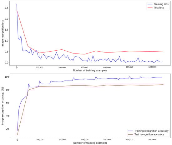
Figure 3.
Training plots and losses plots for the VGG16 network over 13 epochs, the maximum accuracy reached is 87.99%.
To solve the recognition problem, a program modeled in the Jupiter Notebook environment on the Conda core was used. First, the necessary libraries and the databases on which the network will be tested, noisy or cleared, must be downloaded. When the VGG16 architecture was loaded, the last line layer was changed to match the 10 classification classes, and the weights of the architecture network trained on CIFAR10 were imported. The network was trained on an HP Laptop 15s-fq1xxx with an Intel(R) Core(TM) i5-1035G1 CPU @ 1.00 GHz 1.20 GHz, 8.00 GB RAM and a 64-bit operating system. Full-color images 32 × 32 are fed to the input of the first convolutional layer. The next step involved image processing with several convolution layers with 3 × 3 receptive fields. This choice was due to the fact that this is the smallest filter size for determining orientations in the image. Next in the architecture are three fully connected layers, two with 4096 channels each and one with 10 channels by the number of dataset output classes. Accordingly, the soft-max layer performed the classification. All hidden layers were equipped with ReLU. The network did not contain a normalization layer to reduce memory consumption and training time. Also, when testing an actual assembled base, it is necessary to load a file with classes in order to display names instead of class numbers. Then, the testing process takes place on the loaded image database and the result is given as a percentage, by using the confusion matrix.
Table 3 shows the recognition results of the CIFAR10 test bases. The proposed method showed good results in image cleaning. It should be noted that at 1% noise, images during recognition show an accuracy higher than known methods, which is explained by a greater degree of image blur when cleaning noise with these methods.
Table 3.
Comparison of the recognition accuracy of a noisy and cleaned by different methods image database CIFAR 10.
Various criteria and metrics were used to assess the recognition accuracy of the image database:
- F1score is calculated as:where —true positive result, —false positive result and —false-negative recognition result. The range of F1 is in [0, 1] where 1 is the ideal classification.
- The Matthews Correlation Coefficient (MCC) belongs to the range [−1, 1] and has the form:where —true-negative recognition result.
Confusion matrices for the recognition of the CIFAR10 base, noisy with 25% random-valued impulse noise, are shown in Figure 4. The matrix corresponding to the noisy image base shows that the neural network was not able to qualitatively recognize objects in the images. This confirms the importance of image preprocessing before loading into the neural network classifier.
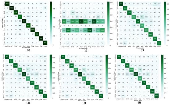
Figure 4.
Comparison of recognition results of original and cleaned from 25% random-valued impulse noise images of CIFAR10 test database: (a) original database recognition accuracy is 87.99%; (b) accuracy of 25% noised database is 17,31%; (c) accuracy of denoised base by [28] is 67.87%; (d) accuracy of denoised base by [27] is 72.99%; (e) accuracy of denoised base by [25] is 73.08%; (f) accuracy of denoised base by proposed method is 74.25%.
Table 4, Table 5, Table 6 and Table 7 present the values of the F1score criterion and the Matthews correlation coefficient obtained by cleaning images from random-valued impulse noise of different intensities. The results reflect that the higher quality of image cleaning by the proposed method—the recognition accuracy of the cleaned base is higher by 56.94% compared to the noisy image, and also higher by 6.38%, 1.26%, and 1.17% compared to the methods from [25,27,28], respectively. In some areas that use computer vision for image classification, such gains in accuracy of 1.26% and 1.17% can be of great importance.
Table 4.
Criteria and metrics of recognition accuracy of the CIFAR10 base, previously cleared of 1% random-valued impulse noise.
Table 5.
Criteria and metrics of recognition accuracy of the CIFAR10 base, previously cleared of 10% random-valued impulse noise.
Table 6.
Criteria and metrics of recognition accuracy of the CIFAR10 base, previously cleared of 25% random-valued impulse noise.
Table 7.
Criteria and metrics of recognition accuracy of the CIFAR10 base, previously cleared of 50% random-valued impulse noise.
We chose the original “Cat_ Maine_Coon “ image (Figure 5a), we then reduced it to 32 × 32 and noised it with random-valued impulse noise of various intensities. Figure 5, Figure 6, Figure 7 and Figure 8 show the results of the recognition of images noisy with impulse noise, which were cleaned by known methods [25,27,28] and the proposed one. As noted earlier, at 1% noise, the recognition accuracy did not differ by a large amount, from which it is concluded that it does not always make sense to remove noise of such intensity from the image. A noise intensity of 10% had already significantly spoiled the image—the neural network showed the class “deer” for this image even after cleaning with known methods. At 25% noise, the neural network showed similar results, except that the proposed method outperformed the next hypothesized category by only 17.1%. Noise with an intensity of 50% or more could not be completely removed for high-quality recognition by the system, for all cleaning methods could not cope with such an intensity, but such a dense noise very rarely appears when transmitting images. In general, when cleaning by the proposed method, the neural network recognized the image cleaned by the proposed method as being better by 13.62% and higher.
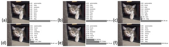
Figure 5.
Results of image “Cat_ Maine_Coon” recognition: (a) original image; (b) image noisy with random-valued impulse noise of intensity 1%; (c) image cleaned by the method [28]; (d) image cleaned by the method [25]; (e) image cleaned by the method [27]; (f) image cleaned by the proposed method.
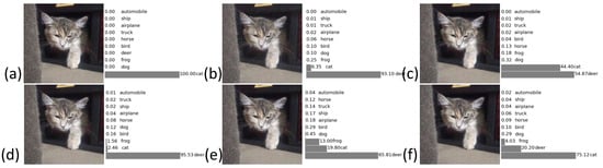
Figure 6.
Results of image “Cat_ Maine_Coon” recognition: (a) original image; (b) image noisy with random-valued impulse noise of intensity 10%; (c) image cleaned by the method [28]; (d) image cleaned by the method [25]; (e) image cleaned by the method [27]; (f) image cleaned by the proposed method.
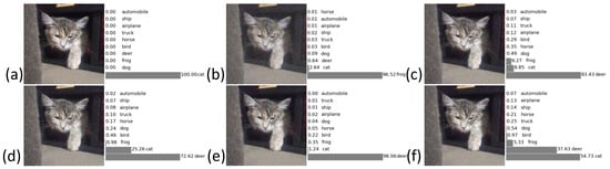
Figure 7.
Results of image “Cat_ Maine_Coon” recognition: (a) original image; (b) image noisy with random-valued impulse noise of intensity 25%; (c) image cleaned by the method [28]; (d) image cleaned by the method [25]; (e) image cleaned by the method [27]; (f) image cleaned by the proposed method.
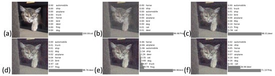
Figure 8.
Results of image “Cat_ Maine_Coon” recognition: (a) original image; (b) image noisy with random-valued impulse noise of intensity 50%; (c) image cleaned by the method [28]; (d) image cleaned by the method [25]; (e) image cleaned by the method [27]; (f) image cleaned by the proposed method.
4. Discussion
The results of recognition of the test, noisy and cleared CIFAR10 bases, showed good results of image cleaning by the proposed method, which directly affected the ability of the neural network to correctly classify the image—from 1.16% to 14.95% recognition accuracy advantage over known methods. It is noted that at 1% of the noise intensity, the uncleaned image is recognized with a higher percentage of belonging to the class. This is due to the fact that any filtering for the purpose of restoring the image can have some degree of blurring, which can impact the quality of feature extraction by the neural network. With noise intensities of 10% and 25%, the proposed method helped to clean the image for recognition with the highest possible accuracy. Noise with an intensity of 50% or more is quite rare in image acquisition or transmission. The proposed method was able to cope with the noise of this intensity visually better than the known methods, but this did not improve the quality of image recognition, as well as in the case of other methods. The results of modeling the recognition of images that fit the category “cat” at a noise intensity of 10% and 25% showed that neither on the noisy nor on the images cleaned by known methods, the neural network was able to identify features to determine belonging to the class, but the image cleared by the proposed method was correctly assigned to the “cat” class. In general, the neural network recognized the original image after cleaning by the proposed method better than after cleaning by known methods. A small difference in the recognition accuracy of cleaned images is not always of great importance, but there are areas where any gain in accuracy is important; for example, in the field of medicine.
5. Conclusions
In the work, a neural network system consisting of a noisy pixel detector, an image cleaning system, and a neural network for image recognition and classification was developed and tested. The problem of determining and removing random-valued impulse noise was solved, which confirms the high accuracy of recognition of cleaned images by a neural network. The high recognition accuracy of the image database cleaned by the proposed method shows the advantage of using such a system in any area. The accuracy increased to 14.95% in some cases, which can be of great importance when solving an applied concern. In the case of solving the difficulty of recognition of one noisy and cleaned image, the proposed system increased the accuracy to 30.72% compared to known methods. It was found that, in most cases, noise with an intensity of 1% does not make it difficult to select a feature map, and it does not make sense to remove it from all images, since the borders are blurred during filtering, which can complicate classification. Noise with an intensity of 50% or more in images is not always possible to remove completely, which affects the quality of class feature extraction by a neural network.
The results of this work can be applied in various areas. In medicine, recognition accuracy is very important for correct and timely diagnoses. In unmanned vehicles, object recognition makes it possible to correctly identify obstacles and quickly respond to them. In the case of data transmission over various communication channels, where they can be affected by noise, the developed system can help not only to qualitatively clean images from noise, but also to recognize noise with high accuracy, even if it is impossible to completely remove noise.
Author Contributions
Conceptualization, A.O., P.L. and V.B.; methodology, A.O., P.L. and V.B.; software, A.O. and V.B.; validation, A.O. and V.B.; formal analysis, V.B.; investigation, A.O., P.L., V.B. and D.K.; resources, A.O. and V.B.; data curation, V.B. and D.K.; writing—original draft preparation, V.B.; writing—review and editing, A.O., P.L., V.B. and D.K.; visualization, V.B.; supervision, P.L.; project administration, D.K.; funding acquisition, P.L. All authors have read and agreed to the published version of the manuscript.
Funding
The research in Section 3.1 was supported by the Russian Science Foundation (Project No. 21-71-00017). Other sections were funded by North-Caucasus Center for Mathematical Research under agreement No. 075-02-2022-892 with the Ministry of Science and Higher Education of the Russian Federation.
Institutional Review Board Statement
Not applicable.
Informed Consent Statement
Not applicable.
Data Availability Statement
Not applicable.
Acknowledgments
The authors would like to thank the North Caucasus Federal University for their support in the project competitions of scientific groups and individual scientists of the North Caucasus Federal University.
Conflicts of Interest
The authors declare no conflict of interest.
References
- Pawlicki, M.; Kozik, R.; Choraś, M. A Survey on Neural Networks for (Cyber-) Security and (Cyber-) Security of Neural Networks. Neurocomputing 2022, 500, 1075–1087. [Google Scholar] [CrossRef]
- Fiore, U. Neural Networks in the Educational Sector: Challenges and Opportunities. In Proceedings of the Balkan Region Conference on Engineering and Business Education, Sibiu, Romania, 16–19 October 2019; Volume 3, pp. 332–337. [Google Scholar] [CrossRef]
- Syam, N.; Kaul, R. Neural Networks in Marketing and Sales. In Machine Learning and Artificial Intelligence in Marketing and Sales; Emerald Publishing Limited: Bingley, UK, 2021; pp. 25–64. [Google Scholar] [CrossRef]
- Romero, J.; Machado, P. Neural Networks in Art, Sound and Design. Neural Comput. Appl. 2020, 33, 1. [Google Scholar] [CrossRef]
- Kumar, V.S.; Gogul, I.; Raj, M.D.; Pragadesh, S.K.; Sebastin, J.S. Smart Autonomous Gardening Rover with Plant Recognition Using Neural Networks. Procedia Comput. Sci. 2016, 93, 975–981. [Google Scholar] [CrossRef]
- Sajna Tasneem, S.; Shabeer, S. Optimized Image Restoration Based on Residual Cascade Convolution Neural Networks. In Proceedings of the International Conference on Intelligent Computing and Control Systems, Secunderabad, India, 15–17 May 2019; pp. 550–553. [Google Scholar] [CrossRef]
- Lou, G.; Shi, H. Face Image Recognition Based on Convolutional Neural Network. China Commun. 2020, 17, 117–124. [Google Scholar] [CrossRef]
- Yun, K.; Huyen, A.; Lu, T. Deep Neural Networks for Pattern Recognition. Adv. Pattern Recognit. Res. 2018, 49–79. [Google Scholar] [CrossRef]
- Zhang, J.; Shao, K.; Luo, X. Small Sample Image Recognition Using Improved Convolutional Neural Network. J. Vis. Commun. Image Represent. 2018, 55, 640–647. [Google Scholar] [CrossRef]
- Wu, W.; Li, L.; Yin, J.; Lyu, W.; Zhang, W. A Modular Tide Level Prediction Method Based on a NARX Neural Network. IEEE Access 2021, 9, 147416–147429. [Google Scholar] [CrossRef]
- Wu, Q.; Jiang, Z.; Hong, K.; Liu, H.; Yang, L.T.; Ding, J. Tensor-Based Recurrent Neural Network and Multi-Modal Prediction with Its Applications in Traffic Network Management. IEEE Trans. Netw. Serv. Manag. 2021, 18, 780–792. [Google Scholar] [CrossRef]
- Chakraborty, R.; Hasija, Y. Predicting MicroRNA Sequence Using CNN and LSTM Stacked in Seq2Seq Architecture. IEEE/ACM Trans. Comput. Biol. Bioinform. 2020, 17, 2183–2188. [Google Scholar] [CrossRef]
- Seo, H.; Bassenne, M.; Xing, L. Closing the Gap between Deep Neural Network Modeling and Biomedical Decision-Making Metrics in Segmentation via Adaptive Loss Functions. IEEE Trans Med. Imaging 2021, 40, 585–593. [Google Scholar] [CrossRef]
- Wang, S.; Archer, N.P. A Neural Network Based Fuzzy Set Model for Organizational Decision Making. IEEE Trans. Syst. Man Cybern. Part C Appl. Rev. 1998, 28, 194–203. [Google Scholar] [CrossRef]
- Wu, Q.X.; McGinnity, M.; Bell, D.A.; Prasad, G. A Self-Organizing Computing Network for Decision-Making in Data Sets with a Diversity of Data Types. IEEE Trans Knowl. Data Eng. 2006, 18, 941–953. [Google Scholar] [CrossRef]
- Steur, N.A.K.; Schwenker, F. Next-Generation Neural Networks: Capsule Networks with Routing-by-Agreement for Text Classification. IEEE Access 2021, 9, 125269–125299. [Google Scholar] [CrossRef]
- Schaller, H.N. Problem Solving by Global Optimization: The Rolling-Stone Neural Network. Proc. Int. Jt. Conf. Neural Netw. 1993, 2, 1481–1484. [Google Scholar] [CrossRef]
- Khaw, H.Y.; Soon, F.C.; Chuah, J.H.; Chow, C.O. Image Noise Types Recognition Using Convolutional Neural Network with Principal Components Analysis. IET Image Process. 2017, 11, 1238–1245. [Google Scholar] [CrossRef]
- Yim, J.; Sohn, K.-A. Enhancing the Performance of Convolutional Neural Networks on Quality Degraded Datasets. In Proceedings of the International Conference on Digital Image Computing, Sydney, Australia, 29 November–1 December 2017. [Google Scholar]
- Zhang, Z.; Han, D.; Dezert, J.; Yang, Y. A New Adaptive Switching Median Filter for Impulse Noise Reduction with Pre-Detection Based on Evidential Reasoning. Signal Process. 2018, 147, 173–189. [Google Scholar] [CrossRef]
- Mújica-Vargas, D.; de Jesús Rubio, J.; Kinani, J.M.V.; Gallegos-Funes, F.J. An Efficient Nonlinear Approach for Removing Fixed-Value Impulse Noise from Grayscale Images. J. Real-Time Image Process. 2018, 14, 617–633. [Google Scholar] [CrossRef]
- Lone, M.R.; Khan, E. A Good Neighbor Is a Great Blessing: Nearest Neighbor Filtering Method to Remove Impulse Noise. J. King Saud Univ. Comput. Inf. Sci. 2022, 34, 9942–9952. [Google Scholar] [CrossRef]
- Singh, A.; Sethi, G.; Kalra, G.S. Spatially Adaptive Image Denoising via Enhanced Noise Detection Method for Grayscale and Color Images. IEEE Access 2020, 8, 112985–113002. [Google Scholar] [CrossRef]
- Momeny, M.; Latif, A.M.; Agha Sarram, M.; Sheikhpour, R.; Zhang, Y.D. A Noise Robust Convolutional Neural Network for Image Classification. Results Eng. 2021, 10, 100225. [Google Scholar] [CrossRef]
- Garnett, R.; Huegerich, T.; Chui, C.; He, W. A Universal Noise Removal Algorithm with an Impulse Detector. IEEE Trans Image Process. 2005, 14, 1747–1754. [Google Scholar] [CrossRef] [PubMed]
- Tomasi, C.; Manduchi, R. Bilateral Filtering for Gray and Color Images. In Proceedings of the IEEE International Conference on Computer Vision, Bombay, India, 7 January 1998; pp. 839–846. [Google Scholar] [CrossRef]
- Dong, Y.; Chan, R.H.; Xu, S. A Detection Statistic for Random-Valued Impulse Noise. IEEE Trans Image Process. 2007, 16, 1112–1120. [Google Scholar] [CrossRef] [PubMed]
- Xiao, X.; Xiong, N.N.; Lai, J.; Wang, C.D.; Sun, Z.; Yan, J. A Local Consensus Index Scheme for Random-Valued Impulse Noise Detection Systems. IEEE Trans Syst. Man Cybern. Syst. 2021, 51, 3412–3428. [Google Scholar] [CrossRef]
- Kumar, S.; sen Yadav, J.; Kurmi, Y.; Baronia, A. An Efficient Image Denoising Approach to Remove Random Valued Impulse Noise by Truncating Data inside Sliding Window. In Proceedings of the 2nd International Conference on Data, Engineering and Applications, IDEA 2020, Bhopal, India, 28–29 February 2020. [Google Scholar]
- Lin, C.; Li, Y.; Feng, S.; Huang, M. A Two-Stage Algorithm for the Detection and Removal of Random-Valued Impulse Noise Based on Local Similarity. IEEE Access 2020, 8, 222001–222012. [Google Scholar] [CrossRef]
- Lin, C.; Qiu, C.; Wang, W.; Zhou, H.; Feng, S.; Huang, M. A New Denosing Method Based on Local Similarity for Removing Impulse Noise. In Proceedings of the Proceedings of 2021 5th Asian Conference on Artificial Intelligence Technology, ACAIT 2021, Haikou, China, 29–31 October 2021. [Google Scholar]
- Hamid, M.M.; Fathi Hammad, F.; Hmad, N. Removing the Impulse Noise from Grayscaled and Colored Digital Images Using Fuzzy Image Filtering. In Proceedings of the 2021 IEEE 1st International Maghreb Meeting of the Conference on Sciences and Techniques of Automatic Control and Computer Engineering, MI-STA 2021, Tripoli, Libya, 25–27 May 2021. [Google Scholar]
- Lyakhov, P.A.; Voznesensky, A.S.; Shalugin, E.D.; Orazaev, A.R.; Baboshina, V.A. Bilateral and Median Filter Combination for High-Quality Cleaning of Random Impulse Noise in Images. In Proceedings of the 11th Mediterranean Conference on Embedded Computing, MECO 2022, Budva, Montenegro, 7–11 June 2022. [Google Scholar] [CrossRef]
- Nazaré, T.S.; da Costa, G.B.P.; Contato, W.A.; Ponti, M. Deep Convolutional Neural Networks and Noisy Images. In Progress in Pattern Recognition, Image Analysis, Computer Vision, and Applications; Lecture Notes in Computer Science, Including Subseries Lecture Notes in Artificial Intelligence and Lecture Notes in Bioinformatics; Springer: Cham, Switzerland, 2018; Volume 10657, pp. 416–424. [Google Scholar]
- Schaefferkoetter, J.; Yan, J.; Ortega, C.; Sertic, A.; Lechtman, E.; Eshet, Y.; Metser, U.; Veit-Haibach, P. Convolutional Neural Networks for Improving Image Quality with Noisy PET Data. EJNMMI Res. 2020, 10, 105. [Google Scholar] [CrossRef] [PubMed]
- Cao, Y.; Fu, Y.; Zhu, Z.; Rao, Z. Color Random Valued Impulse Noise Removal Based on Quaternion Convolutional Attention Denoising Network. IEEE Signal Process. Lett. 2022, 29, 369–373. [Google Scholar] [CrossRef]
- Jang, H.; McCormack, D.; Tong, F. Noise-Trained Deep Neural Networks Effectively Predict Human Vision and Its Neural Responses to Challenging Images. PLoS Biol. 2021, 19, e3001418. [Google Scholar] [CrossRef]
- Konar, D.; Gelenbe, E.; Bhandary, S.; das Sarma, A.; Cangi, A. Random Quantum Neural Networks (RQNN) for Noisy Image Recognition. arXiv 2022, arXiv:2203.01764. [Google Scholar]
- Keohane, O.; Aizenberg, I. Impulse Noise Filtering Using MLMVN. In Proceedings of the International Joint Conference on Neural Networks, Glasgow, UK, 19–24 July 2020. [Google Scholar]
- Kim, T.H. Pattern Recognition Using Artificial Neural Network: A Review. Commun. Comput. Inf. Sci. 2010, 76, 138–148. [Google Scholar] [CrossRef]
- Bickel, P.J.; Doksum, K.A. Mathematical Statistics: Basic Ideas and Selected Topics; CRC Press: Boca Raton, FL, USA, 2015; ISBN 9781498723800. [Google Scholar]
- Aggarwal, C.C. Neural Networks and Deep Learning. In Neural Networks and Deep Learning; Springer: New York, NY, USA, 2018. [Google Scholar] [CrossRef]
- Nadeem, M.; Hussain, A.; Munir, A.; Habib, M.; Naseem, M.T. Removal of Random Valued Impulse Noise from Grayscale Images Using Quadrant Based Spatially Adaptive Fuzzy Filter. Signal Process. 2020, 169, 107403. [Google Scholar] [CrossRef]
- George, G.; Oommen, R.M.; Shelly, S.; Philipose, S.S.; Varghese, A.M. A Survey on Various Median Filtering Techniques For Removal of Impulse Noise From Digital Image. In Proceedings of the IEEE Conference on Emerging Devices and Smart Systems, ICEDSS 2018, Tiruchengode, India, 2–3 March 2018. [Google Scholar]
- Lan, X.; Zuo, Z. Random-Valued Impulse Noise Removal by the Adaptive Switching Median Detectors and Detail-Preserving Regularization. Optik 2014, 125, 1101–1105. [Google Scholar] [CrossRef]
- Lyakhov, P.A.; Orazaev, A.R.; Chervyakov, N.I.; Kaplun, D.I. A New Method for Adaptive Median Filtering of Images. In Proceedings of the 2019 IEEE Conference of Russian Young Researchers in Electrical and Electronic Engineering, ElConRus 2019, Moscow, Russia, 28–31 January 2019; pp. 1197–1201. [Google Scholar] [CrossRef]
- Chervyakov, N.I.; Lyakhov, P.A.; Orazaev, A.R. 3d-Generalization of Impulse Noise Removal Method for Video Data Processing. Comput. Opt. 2020, 44, 92–100. [Google Scholar] [CrossRef]
- Cui, H.; Xiong, R.; Luo, C.; Song, Z.; Wu, F. Denoising and Resource Allocation in Uncoded Video Transmission. IEEE J. Sel. Top. Signal Process. 2015, 9, 102–112. [Google Scholar] [CrossRef]
- Simonyan, K.; Zisserman, A. Very Deep Convolutional Networks for Large-Scale Image Recognition. In Proceedings of the 3rd International Conference on Learning Representations, ICLR 2015—Conference Track Proceedings 2014, San Diego, CA, USA, 7–9 May 2015. [Google Scholar] [CrossRef]
- Krizhevsky, A.; Sutskever, I.; Hinton, G.E. ImageNet Classification with Deep Convolutional Neural Networks. Commun. ACM 2017, 60, 84–90. [Google Scholar] [CrossRef]


Disclaimer/Publisher’s Note: The statements, opinions and data contained in all publications are solely those of the individual author(s) and contributor(s) and not of MDPI and/or the editor(s). MDPI and/or the editor(s) disclaim responsibility for any injury to people or property resulting from any ideas, methods, instructions or products referred to in the content. |
© 2023 by the authors. Licensee MDPI, Basel, Switzerland. This article is an open access article distributed under the terms and conditions of the Creative Commons Attribution (CC BY) license (https://creativecommons.org/licenses/by/4.0/).