Paper Tissue Softness Rating by Acoustic Emission Analysis

Abstract

Softness is one of the essential properties of hygiene tissue products. Reliably measuring it is of utmost importance to ensure the balance between customer expectations and cost-effective tissue production. This study presents a method for assessing softness by analyzing acoustic emissions produced while tearing a tissue specimen. The aim was to train neural network models using the corrected results of human panel tests as the ground truth labels and to predict the tissue softness in two- and three-class recognition tasks. We also investigate the possibility of predicting some production parameters related to the softness property. The results proved that tissue softness and production parameters could be reliably estimated only by the tearing noise.

1. Introduction

The hygiene tissue market is growing [1] with the most significant amount of tissue paper products consumed in East Asia, North America, and Europe [2]. Tissue is a particular type of paper used in daily hygiene, such as table napkins, toilet paper, kitchen towels, cosmetic tissues, and industrial wipes [3]. Depending on the intended product end use, specific physical attributes of tissue products (such as softness, strength, fluid absorbency, and bulkiness) are targeted in the production, closely linked to the machine technologies, fiber types and the chemical additives [4].

One of the essential properties of hygiene tissue products for consumers is their softness. Therefore, properly assessing these properties is of utmost importance for hygiene tissue production. Softness as a sensory characteristic can be defined as a complex set of inputs, including appearance, mechanical properties (bulk), friction properties (smoothness), vibration characteristics, and sound [1].

Consumers will not prefer a tissue that does not meet the expected level of perceived softness and smoothness (too rough or unpleasant). Furthermore, they place high demands on the softness in hygiene tissues in contrast to other materials or papers of higher strength. On the one hand, tissues that are too soft arouse higher demands from the customer, but, on the other hand, such product is expensive to produce. Therefore, a reliable measurement method is necessary to balance the softness and the production costs. It is not yet possible to give an objective and quantitative measure of the respective softness, as is possible, for example, for strength or water absorption capacity.

The widely accepted method for softness assessment is the panel test, where trained panelists perceive the softness by gently rubbing the fingertips and palms over the tissue surface (surface softness) or by folding and crumpling a tissue (bulk softness). The panelists are asked to grade the softness of sample tissues on a specific scale against the reference samples with fixed scores (scoring method). Another way to evaluate is where the panelists are asked to rank the tissue samples from least to most soft by a pair-wise comparison (ranking method). However, softness as subjective perception is difficult to define and quantify, and the panel tests are a time and cost-intensive process, particularly in the case of a large number of samples with fewer references [5].

A factor that further complicates the softness assessment is that many tissue manufacturers do not publish their evaluation procedures. The test parameters could differ only slightly, but comparability among them is impossible. Recently, many analytical methods were developed to instrumentally quantify the paper properties, which can be used individually or in combination to correlate with softness. For instance, strength, stiffness, and softness typically depend on sheet density and creping geometry; therefore, exploring the correlation between the physical properties contributes to reliable softness modeling.

An extensive overview of the tissue softness measurements is given in [1], divided into Direct Measures of Softness, Prediction Models for Correlating with Softness, and Indication of Surface Topography. Recent advances use a combined approach of custom softness measurement equipment and integrated algorithms that effectively characterize softness, especially after calibration.

The idea, that acoustic emission analysis (AE) can characterize the paper’s physical properties during the destruction of the fiber-to-fiber bonds, the fiber, or the fiber deformation, has been present for a long time [6]. Many studies showed that the different fiber types produce different sound frequencies, and the frequency analysis shows that weak bonds are loosened first, then the stronger bonds, and in the end, the fibers [7]. Papers with increased latex content show higher strength combined with a slight increase in acoustic emissions [8]. In the study [9], the authors investigated the micro mechanics behind the behavior of paper under mechanical loading by AE monitoring that was used for detecting and recording damage. In [10], statistical analysis of acoustic emission data from tensile experiments on paper sheets was conducted, with samples broken under strain control. In [11], acoustic emissions were used to investigate the development of damage in paper specimens. The preliminary study [12] investigated the possibility of distinguishing between different types of paper towels by analyzing the tearing noise. Hidden Markov Models were trained on sounds of five different types of papers, and approximately $75\%$ of the samples were correctly recognized.

The acoustic emission also can be produced by converting vibrations caused by friction of the fabric surface into an acoustic spectrum. The tissue softness analyzer (TSA) [13] measures three decisive properties: fiber softness (TS7), texture (TS750), and stiffness (D). From these measured variables, as well as thickness, grammage, and the number of plies, a hand-feel (HF) value is calculated using mathematical models.

Several studies [14,15] compared TSA hand-feel measurement to panel tests and found a strong linear correlation between TSA-HF and panel tests. The TS7 parameter, which measures the surface softness, has the strongest linear correlation with the panel tests [16].

This paper presents a machine-learning approach that uses acoustic emissions produced by tearing paper tissues for softness assessment. Acoustic emission with machine learning is widely used in manufacturing, structural health monitoring, product quality control, and material research [17]. However, to the best of our knowledge, there are no comparable studies investigating the classification of acoustic emissions of paper tissue products using deep learning.

The binary and three-class recognition results showed that reliable estimation of tissue softness (surface and bulk) with end-to-end Convolutional Neural Networks (CNN) is practically feasible, despite the small amount of collected audio samples. Moreover, the same approach was successfully applied for multi-class recognition of separate production parameters and their combination as a tissue type and post-production of physical properties. Therefore, such models can also be employed for quality control by monitoring any deviation from the tissue production specification.

The paper is structured as follows: Section 2 describes the used paper tissue types and their production parameters, the organization of the panel tests, exploratory statistics, data collection, and acoustic properties. Section 3 presents the experimental setup, used performance metrics, and the machine learning methods. The results and the discussions are given in Section 4. We conclude the paper with Section 5.

2. Materials and Methods

2.1. Materials

Paper tissues originating from 42 tambours were used for the panel tests, with an additional one as the “good” standard. Each tambour has its own unique identification.

Table 1. Production and physical properties of tissues.

			Tissues
Type	B028	B053	B348	BX 068	BX068	DS 002	DX062
#Tambours	5	5	6	6	7	6	5
			Parameters
Caima	4	7	5	5	5	10	10
Caima + Ponteverde	13	14	5	13	13	10	18
Creping factor	20.5	18.5	18.5	16.5	17.5	18.5	17.5
			Properties
Stretching [%]	22.8	23.4	18.2	31.6	31.6	9.1	13.5
Surface mass [g/m${}^2$]	15.6	15.6	15.9	15.9	15.6	15.6	15.5

shows the counts of the tambours by the tissue type determined by manufacturing parameters, such as “Creping factor“, pulp type contribution to fiber composition (“Caima”, “Caima + Ponteverde”), and physical properties of the product, such as the relative stretching length before tearing and the surface mass. Some parameters could have slight variations (rollers’ rotation speed, humidity), but the critical ones were kept constant during production.

2.2. Panel Tests

This study aims to predict the softness of a paper tissue originating from an unknown tambour in the form of a softness score. All individual paper grades were ranked for softness with pair-wise comparison in a panel test (6 panelists) and then normalized to an Elo scale [18].

Elo ranking system is devised for calculating the relative skill levels of two competitors in zero-sum games (such as chess) [19], and it is also applicable in this case where two paper grades (of different tambours) are “competing” to win the “softer than the other” game. The difference to the traditional Elo system is that there is no “draw” outcome in this case, so one tissue sample will always be perceived as softer.

The achieved results represent the most probable ranking. The Elo number is a measure of softness, i.e., a softness rating number (the higher, the softer). It has the character of a mean value, and thus, assuming a symmetrical distribution (e.g., Gaussian), it is also the most likely rating number.

The absolute values in the ranking are irrelevant; only the rating differences matter. The $95\%$ confidence intervals were calculated according to the number of comparisons that varied between 35 and 56, with an average of 50. Additional values are the score that indicates the percentage point yield achieved (1 point for win, 0 for loss) and Average Opponent Rating (Av.Op.) indicates the rating average of the “opponents” against whom this score was achieved.

We defined three softness classes (good, medium, and poor) for the classification based on the Elo rankings. The task of the classification system is to determine the correct class of a paper grade unknown to it. The class division was set so that all categories had the exact count of paper grade samples. Classification in terms of “good” and “poor” standard paper grades was also explored, although the imbalanced class problem had to be considered.

To compare the automatic classifier with the panel tester’s recognition performance, the tester agreement rate was determined, and the reference recognition rate was set to approximately $60\%$ with the random guess baseline of $33\%$ (in the case of 3 balanced classes).

2.3. Exploratory Statistics

We compiled the information about the tambours, the production process, and the resulting physical properties into a dataset. The results of the panel tests in terms of Elo scores and the assigned tissue softness classes are also included.

The bias in the panel tests and the criteria of division in three softness classes governed only by the class balance requirement introduced different labels assigned to tambours produced using the same manufacturing parameters.

Since the parameters influencing the softness did not change during production, we corrected the softness labels belonging to the same paper type for all affected tambours according to the majority vote of the panel testers.

We employed linear regression modeling to discover which of the production parameters (“Caima” (C), “Caima + Ponteverde” (CP), and “Creping factor” (K)) are significant predictors for the tissue softness described by the Elo scores, panel test classes and corrected classes. Instead of ordinal, the classes are considered continuous variables indicating the level of tissue softness.

As expected, the three classes derived from the panel test could not be modeled by the production parameters, providing only an Adjusted R-squared of $0.1501$ and no significant independent variables.

However, Elo scores yielded a loose fit with an adjusted R-squared of $0.5227$, and the CP ($p<0.001$) and K ($p<0.001$) as significant predictors.

Consequently, in the case of corrected panel test labels, it was only confirmed that the CP ($p<0.001$) and K ($p<0.001$) are the significant predictors for tissue softness, with an adjusted R-squared of $0.8509$ (the case of three softness class) and adjusted R-squared of $0.8712$ in the case of binary class regression.

Regarding the percent of stretching as a measurable property, it also has the CP and K as significant predictors ($p<0.001$) with an adjusted R-squared of $0.8606$.

These results indicate that the tissue softness is highly dependent on the two production parameters: increasing the amount of “Caima + Ponteverde” (CP) in the fiber composition and decreasing the “Creping factor” (K). These findings only confirmed the manufacturer’s indications about these two parameters’ influence on the softness.

2.4. Data Collection

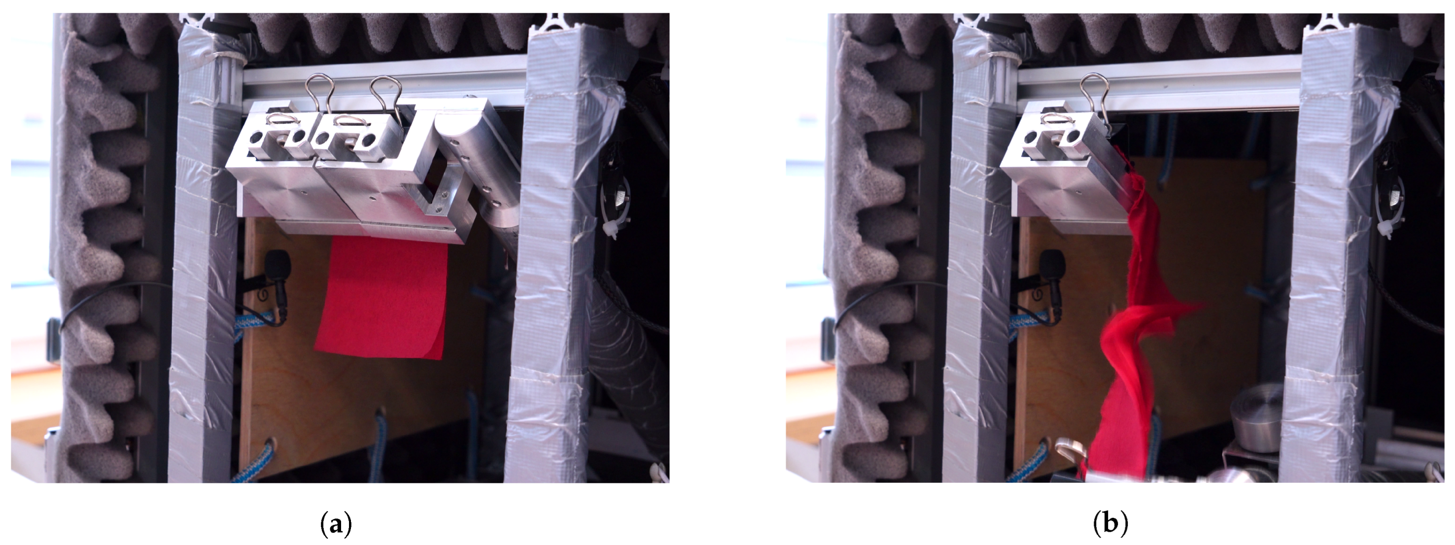
A prototype device was built (Figure 1) to record a paper tissue’s acoustic emissions of tearing sound [20]. It consists of a soundproof enclosure (PROEL Combo Case-6U, ${19}^{″}$) which is 545 mm × 687 mm, lined with soft polyurethane foam (10 mm base and 30 mm pyramid size) and rubber feet for optimal acoustic insulation. The tearing mechanism is constructed according to the Elmendorf principle [21], where the tearing is produced by two separated parallel handles on which the specimen is clamped. One handle is fixed to the casing, and the other is movable. A magnet holds the mechanism, and the movable hand is released at the push of a button and drops, tearing the specimen. The release path is 150 mm, resulting in a tear length of approximately 75 mm. The audio recording equipment consists of an MK301E microphone, an MV310 microphone amplifier, an 8-channel M208A amplifier, and an NI-USB-4431 measurement system. Such a setup ensures consistent tearing of the tissues where the microphone(s) record the produced sound. The microphone is located as close as possible to the source of the tearing noise while attached to the casing by a “Microphone spider” effectively insulating it from the structure-borne noise.

One operator used the prototype to record tearing sounds of 44 tissue grades from different tambours (43 from the panel test and both reference tissue grades), resulting in a total of 2048 recordings. The audio recordings have a duration of 2 s, containing segments with initial silence, the tissue tearing noise, and the noise of the mechanical device, followed again with silence. The minimal count of samples was 38, and the maximum was 52, with a mean value of 48.8 recordings per tambour. The raw input signals are automatically segmented to the interval from 0.1 to 0.6 s that contain only the tearing noise, and they have a fixed length of 48,000 samples.

2.5. Acoustic Properties

We investigated the variations in the Fast Fourier Transform (FFT) spectra in terms of median, first, and third quartiles of the amplitudes for the segmented signals (Figure 2a) and the last 10% of the duration of the original signal containing background noise (Figure 2b). In the FFT analysis, we used a Blackman window with a length of 48,000. The DC offset and the effects of the anti-aliasing filter from the measurement equipment are also visible. The DC offset is omitted in the subsequent feature analysis.

After visual inspection of the FFT spectra variations of the “good” and the “poor” samples, we concluded that there are, in general, minor differences visible in the frequency domain. The differences appear for the higher frequencies (over 12 kHz), which could be explained as the noise of breaking fine-fiber bonds of “good” tissue samples. Such differences are not present in the background noise spectra ruling out any introduced bias in the tissue tearing experiments. However, the observed differences in the frequency domain are subtle and inconsistent, not helping reliable differentiation of “good” and ”poor” tissue softness.

Additionally, we qualitatively analyzed the acoustic properties of typical but single examples of a “good” and a “poor” tissue sample, where the good and the poor standard are defined by the panel tests. The raw signal waveform shows that the “poor” standard exhibits longer periods of larger amplitudes (Figure 3b) after the initial tear sound than the “good” standard (Figure 3a). The amplitude unit is the normalized voltage (NV) from the measurement system.

The criterion that could be used to distinguish the “good” and “poor” standard signals in the time-frequency domain is two-fold, influenced by the magnitude levels and the ripple frequency.

In most cases, the “good” standard tissue produced a tearing sound with lower variations in the amplitudes of frequency spectra over time (Figure 4a), observed as more frequent but less pronounced ripples on the spectrogram with larger magnitude for higher frequencies. Contrary to the “good” standard, the ripples in the spectrogram for the “poor” standard were more emphasized and occurred at longer time intervals (Figure 4b).

The parameters of the spectrogram analysis are short-time Fourier transformation with a Blackman window of 512 ($5.33$ ms), the frame rate of 160 ($1.66$ ms) samples, and MEL filter-bank with a triangular transfer function providing high fidelity visualization and capturing fine details of the time-frequency domain. The spectrograms have a dimension of $289\times 30$.

The effects visible on the spectrogram can be explained as follows: the tissue with lower softness consists of stronger bonds that should be broken, needing more energy that causes larger amplitude and time variations (ripples) in the emitted sound.

After an exploratory analysis with a Principal Component Analysis (PCA) and twodimensional scatter plots of both reference recordings, we observed an overlap in the data point clusters, indicating that the parameters of the feature analysis might not be most suitable.

3. Experimental Setup

This study aims to train a model using the corrected results of the panel tests (Section 2.3) as the ground truth labels and to predict the tissue softness of an unknown tambour, which recordings were not used in training. The classes with labels “poor” and “medium” softness were merged for the binary classification.

To avoid any bias introduced during tambour production and the recording sessions, a repeated stratified group K-fold cross validation (CV) was used with five folds. The CV was repeated five times within the same process to improve the statistical significance of the results. The folds contain non-overlapping groups of tambours. That provided that each group appeared exactly once in the test set across the folds.

Figure 5a presents one repetition of the stratified group 5-fold CV, where from 42 groups—$20\%$ are selected (8 or 9, depending on the repetition-fold run) for the test set keeping the approximate class count ratio, the rest is used for model training per repetition-fold run.

We also investigate the possibility of predicting some of the production parameters that influenced the softness of the tissue product. In this case, we used the repeated stratified K-fold (CV) strategy without considering groups.

Because of the adopted CV strategy, in the case of the tissue softness prediction with two or three classes, the number of training samples was not always $80\%$ of the total sample count (2048), and it varied between 1609 and 1656. In the prediction of the production parameters, it was either 1638 or 1639 samples.

Setting the same seed for the random generator ensured reproducible results of the experiments.

Due to the imbalanced classes in the training set, class weights were applied to different classifiers to avoid creating biased models.

Figure 5b presents the model training per repetition-fold run for three-class recognition and subsequent prediction on the test data for performance evaluation. Both examples presented on Figure 5 are analogous to the binary classification case.

3.1. Performance Metrics

Since our dataset is imbalanced ($26\%$ “poor”, $17\%$ “medium” and $57\%$ “good” standard), evaluation with the accuracy rate and F-score only would produce biased results [22]. Therefore we use the posterior balanced accuracy rate [23,24] and, additionally to the F-score, the Matthews Correlation Coefficient (MCC) [25] as more appropriate performance indicators.

The accuracy rate for each class i (the recall) is defined as [26]:

$$A_i=\frac{C_i}{N_i},i\in \{0,1\},$$

(1)

where $N_i=\left|{\mathcal{D}}_i\right|$ is the total number of samples and $C_i$ is the number of correctly classified samples for class $c_i$. According to [23], the posterior distribution of the class accuracy rate $A_i$ can be expressed as a Beta distribution with parameters ${\alpha }_i$ and ${\beta }_i$:

$$\left(A_i\right|C_i)\sim \mathrm{Beta}({\alpha }_i,{\beta }_i),i\in \{0,1\},$$

(2)

where ${\alpha }_i=1+C_i$ and ${\beta }_i=1+N_i-C_i$, and the probability density x of correctly classifying unseen samples is:

$$P_{A_i}(x;{\alpha }_i,{\beta }_i)=\frac{\Gamma ({\alpha }_i+{\beta }_i)}{\Gamma \left({\alpha }_i\right)\Gamma \left({\beta }_i\right)}{x}^{{\alpha }_i-1}{(1-x)}^{{\beta }_i-1},i\in \{0,1\}.$$

(3)

The balanced accuracy rate is estimated as the average of individual recalls $\frac{1}{2}(A_0+A_1)$, whose probability density can be estimated by convolution:

$$P_B(x;{\alpha }_0,{\beta }_0,{\alpha }_1,{\beta }_1)={\int }_0^1{P}_{A_0}\left(2(x-y);{\alpha }_0,{\beta }_0\right)·P_{A_1}\left(2y;{\alpha }_1,{\beta }_1\right)dy.$$

(4)

$$BAR=E\left|X\right|={\int }_0^{1}x·P_B\left(x\right)dx$$

(5)

Hence, balanced accuracy is the expected value (5) of the probability density (3). Additionally, we compute the 95% Clopper-Pearson confidence interval (CI) according to [27].

The macro average ($\mu$) and standard deviation ($\sigma$) of the F-scores were calculated over the cross-validation folds and the repetitions. The F-score is defined as the harmonic mean of precision and recall:

$$F\text{-}score=\frac{2tp}{2tp+fp+fn}$$

(6)

where $tp$ are true positives, $fp$ are false positives and $fn$ false negatives. An F-score of $1.0$ means an ideal classifier with perfect precision and recall. For the multi-class task, the one-vs-rest approach calculates the per-class F-score and its average value.

The Matthews Correlation Coefficient metric was employed for all classification tasks, and it is calculated as follows:

$$MCC=\frac{tp\times tn-fp\times fn}{\sqrt{(tp+fp)(tp+fn)(tn+fp)(tn+fn)}}$$

(7)

for the binary case it provides a value between $-1.0$ (random prediction) and $+1.0$ (perfect prediction). For the multi-class task, MCC is generalized by K-class correlation coefficient $R_K$ [28].

To illustrate the binary classification ability, we also calculated the Receiver Operating Characteristic-Area Under the Curve (ROC-AUC), providing values between 0 (inverse) and 1 (ideal classification) where the random classifier has a score of $0.5$.

Since we use the BAR as a metric, we calculated the baseline for the random rate classifier as the inverse of the number of classes, e.g., $50\%$ for binary, $0.33\%$ for three, $0.25\%$ for four classes, and so on.

3.2. Machine Learning Approach

One of the standard deep learning approaches for sound classification is to use a 2D visual representation (spectrogram) estimated from the raw audio signals.

These were used as input in two-dimensional convolutional neural network (CNN) architectures initially designed for image and object recognition [29,30]. A spectrogram describes high-dimensional signals into a more compact representation suitable for the 2D-CNN classifiers. However, the performance of such an approach highly depends on the available training data and the input features’ dimensionality.

Conversely, an end-to-end approach with a convolutional neural network can learn the representations directly from the raw audio signal, reducing the computational costs and the required training data.

In the experiments, we trained 2D-CNN classifiers on spectrograms created as described in Section 2.5. We also employed end-to-end 1D-CNN architecture based on the one presented in [30], which was successfully used for environmental sound classification directly from the audio signal.

The features learned directly from the raw audio signal best describe the differences in the tissue softness, according to the ground truth labels from the panel test. After exploratory trials, we found that the following 1D-CNN topology performs best on our datasets. The input layer accepts pulse code-modulated audio signals with a sample rate of 96 kHz.

Figure 6 presents the overall architecture of the employed CNN models for assessing the softness of paper tissue. The device tears the tissue sample producing acoustic emission noise, which was recorded and converted to a digital audio signal as an input for the 1D-CNN model. The audio signal is also transformed into the time-frequency domain as explained in Section 2.5 as the input for the 2D-CNN model. Along each layer, the number of filters and the dimensions are given. A detailed overview of the 1D-CNN topology is given in

Table 2. 1D convolutional neural network for audio signals.

	CL1	MPL1	CL2	MPL2	CL3
Dim	24,000	3000	1500	188	92
Filter Size	64	8	32	8	16
# Filters	16	16	32	32	64
Stride	2	8	2	8	2

and the following paragraphs.

Similarly, the 2D-CNN topology has two convolutional layers (CL) with 32 filters and kernel sizes of ($11\times 41$) and ($11\times 21$), respectively, a stride of two, followed by a fully-connected layer with 256 nodes. Each layer was batch normalized with a rectified linear unit (ReLU) as the activation function.

In the case of the 1D-CNN, Leaky ReLU was the activation function followed by max-pooling layers (MPL). The convolutional layers provided the input to one fully connected layer with 64 units. In both cases, the architectures have a relatively small amount of trainable parameters (1D-CNN: 435K and 2D-CNN: 10M), which should be appropriate for smaller datasets as in this case. For all the architectures mentioned above, the output layer has a softmax activation function with the output nodes corresponding to the target classes (2–5, 7) and categorical cross entropy as a loss function.

Although using Adadelta and Adagrad is a more appropriate choice in the case of sparse data, in both cases, we used Adam, considered the best optimizer.

To prevent over-fitting, a high dropout ratio rate ($0.5$) on the fully-connected layer is used during training with early stopping criteria of 10 epochs with no improvement in the monitored loss function.

4. Results and Discussion

We conducted the three-class classification experiment with the original (non-corrected) panel test labels, achieving $46.67\%$ BAR, which is below the panel test recognition rate ($60\%$) and the Gaussian Mixture Hidden Markov Models (HMM/GMM) classifier’s performance ($52\%$) as presented in the technical report [31]. The reason is that the ad hoc division in balanced classes not considering the consistency within the paper types (production parameters).

4.1. Tissue Softness Classification

Table 3. Three-class classification performance.

3-Class	BAR (95% CI)	F-Score: $\mathit{\mu }$ ($\mathit{\sigma }$)	MCC
2D-CNN	${73.79}_{-0.50}^{+0.49}$	0.7254 (0.050)	0.6196
1D-CNN	${78.44}_{-0.46}^{+0.46}$	0.7881 (0.047)	0.6840

presents the results in BAR with the 95% confidence intervals, F-score with standard deviation across the folds-repetitions, and the MCC score.

Furthermore, it is observed that the most confusion occurred between the class “poor” and “medium”, indicating that the original data division in classes is not appropriate.

Hence, we repeated the experiments as a binary classification problem to predict if a tissue product has “high” (preferable) or “low” (not preferable) softness.

The results are presented in

Table 4. Binary classification performance.

2-Class	BAR (95% CI)	F-Score: $\mathit{\mu }$ ($\mathit{\sigma }$)	MCC
2D-CNN	${85.96}_{-0.39}^{+0.39}$	0.8574 (0.0526)	0.7164
1D-CNN	${88.40}_{-0.36}^{+0.35}$	0.8751 (0.0619)	0.7699

and the ROC with AUC in Figure 7. It can be seen that the performance improved in terms of BAR, MCC, and F-score for both CNN architectures and that the 1D-CNN with raw signals outperforms the 2D-CNN with spectrogram features.

The probability of misclassification of the tissue softness in repeated trials is exponentially reduced with the number of trials. With N trials on specimens of the same tambour, the error rate (ER) is $ER={(1-BAR)}^N$, for instance, with $N=3$ and $BAR=0.884$ (2-class), the probability that all of the specimens will be misclassified is $ER=0.0016$.

It is also evident that the engineered features (spectrograms) for the 2D-CNN are not optimal. The classification performance is lower than that achieved by 1D-CNN end-to-end classifier. Since optimizing the feature analysis is costly and not feasible, only the 1D-CNN classifiers were employed in the following experiments.

4.2. Production Parameters Recognition

To investigate the influence of separate and joint production parameters (Type), a series of experiments were performed to classify categories of parameters as presented in Table 1.

Here, we employed a different CV strategy and the five times repeated Stratified 5-fold without leaving groups (tambours) out because, in some of the repeated folds, few classes are not present in training.

From

Table 5. Production parameters classification performance.

Parameter (#Class)	F-Score: $\mathit{\mu }$ ($\mathit{\sigma }$)	MCC
Caima (4)	0.7564 (0.0369)	0.6575
Caima + Ponteverde (5)	0.7723 (0.0234)	0.7075
Creping factor (4)	0.7963 (0.0325)	0.7831
Type (7)	0.7577 (0.0246)	0.7226
Stretching (7)	0.7622 (0.0227)	0.7240

and Figure 8, the production parameters that are significant predictors (see Section 2.3) for the tissue softness, “Caima + Ponteverde” and “Creping factor” achieved better classification than “Caima”. The achieved results are better than those presented in the technical report [31] on the same data with the HMM/GMM classifier and engineered features, “Caima” ($BAR=65.4\%$), “Caima + Ponteverde” ($BAR=62.6\%$) and “Creping factor” ($BAR=62.3\%$).

All parameters, except the “Creping factor”, do not exhibit systematic confusion. From the confusion matrix, it can be seen that most errors are divided between the lower and higher values. Therefore this parameter could also be transcribed with only “high/low” labels. The tissue type corresponding to specific production parameter combinations can be recognized reliably, too, as well as the relative stretching length before tearing, as post-production physical property.

5. Conclusions

We presented a methodology for tissue softness assessment by acoustic emission analysis. We recorded the sound of tearing paper tissue, and the data was employed to train neural network models to predict the softness and some production parameters.

Acoustic emission testing with machine learning is widely used in engineering and manufacturing. However, few studies investigate acoustic emission in the production of paper tissue. Machine learning studies are rare, and datasets comparable to ours are unavailable.

We investigated the results of the panel tests and their relation to the production parameters. Consequently, the corrected ranking scores were used as the ground truth to train neural network models that can characterize tissue softness as “good” or “poor”.

We compared our results with those presented in previous works on the same data with similar classification tasks, however, with different pattern recognition approaches. We showed that reliable classification of paper tissue softness and production parameters is possible using end-to-end CNN models trained on a small dataset.

The results indicate that the proposed approach is practically feasible to be used in manufacturing of paper tissue quality monitoring.