1. Introduction
Mechanical troubleshooting is vital for the reliable operation of modern industrial systems. Gearboxes are the main transmission components of industrial equipment that have been widely used in aircraft, wind turbines, automobiles, and other equipment [
1,
2], whereas gearboxes often operate in a complex and harsh working environment for a long time, and their components often work continuously at high speed with heavy load leading to a high failure rate and coupling faults [
3]. Therefore, the study of fault diagnosis methods for gearboxes should be a concern that can prolong the use of machinery and equipment, reduce economic losses, and avoid accidents.
The most effective and direct fault detection method for gearboxes is vibration signal analysis. The existing system diagnostic methods can be divided into two types, namely traditional signal analysis methods and machine learning methods [
4]. Most of the traditional signal analysis methods are based on physical and mathematical principles to extract and detect the fault-related features in the original signal [
5]. However, the working environment of gearboxes is complex, so the vibration signal usually contains information about the characteristics of other components, such as the rotation of shafts and bearings, and the meshing of gears. Moreover, fault coupling of different components may also occur under long-term operation. These factors add difficulties to gearbox fault diagnosis. In addition, the vibration signal of the component associated with the fault is thoroughly weak and can be susceptible to being swamped by other vibrating components in the early stages [
6]. Therefore, traditional signal-based analysis methods are difficult to identify the vibration components associated with a fault.
On the other hand, intelligent fault diagnosis has come a long way with the development of machine learning theory, and prevalent machine learning methods include artificial neural networks (ANN) [
7], support vector machines (SVM) [
8], and k-means method [
9], etc. The intelligent diagnosis steps of machine learning are divided into signal acquisition, feature extraction, and machine learning model classification. However, the difficulty of machine learning fault diagnosis lies in finding an effective feature [
10].
Recently, with the development of artificial intelligence, deep learning (DL) methods have become a practical tool for fault diagnosis based on vibration signals [
11]. Deep learning methods are machine learning methods with multi-level nonlinear transformations. However, in real industrial scenarios, vibration signals collected by the gearbox contain a lot of noise, and excessive noise will drown out the signal that characterizes the fault. In this case, a general DL mode can make a rough judgment. Therefore, minimizing the impact of noise on diagnostic models is the focus of current research. Several researchers have studied intelligent fault diagnosis in environments with strong noise and variable loads. Su et al. [
12] proposed a hierarchical branching CNN (HB-CNN) method with excellent robustness in bearing fault diagnosis, Zhang et al. [
13] proposed a training interference convolutional neural networks (TICNN) method that shows excellent performance in a noisy environment, and Mo et al. [
14] proposed a new method of integrating a learnable variational kernel into a one-dimensional CNN. To further improve the diagnostic performance of the network model, many researchers have given the model a stronger ability to extract features. Yu et al. [
15] proposed a broad convolutional neural network (BCNN) with certain incremental learning abilities. Li et al. [
16] constructed a CNN-BGM model with a mixture of neural networks and Bayesian Gaussians. Jiao et al. [
17] proposed a deeply coupled dense convolutional network (CDCN).
Neural networks are generally optimized by a backpropagation algorithm which updates parameters by the gradient. Some networks obtain better performance by increasing the number of layers of the network, which tends to the disappearance of the gradient, and the underlying parameters cannot be updated. Deep residual networks (ResNet), a popular derivative of convolutional networks, use identity shortcuts to alleviate the difficulty of parameter optimization. In residual networks, optimization of the underlying parameters can be solved because gradients can be imported with identity shortcuts [
18,
19]. Chen et al. [
20] proposed a dual-path mixed-domain residual threshold network (DP-MRTN) to improve the diagnostic performance of rolling bearings in high-noise environments. Li et al. [
21] proposed a one-dimensional residual convolution neural network (1D-RCNN) that directly uses time-domain waveforms as input. Zhao et al. [
22] used a residual network to fuse multiple sets of wavelet packet coefficients for fault diagnosis. Sun et al. [
23] proposed a multi-scale cluster-graph convolution neural network with a multi-channel residual network (MR-MCGCN), which can eliminate the effect of noise efficiently.
Many researchers have found that the vibration signals of gearboxes have inherent multiscale features. Jiang et al. [
24] proposed a new multiscale convolutional neural network (MSCNN) with coarse granularity strategy to effectively learn fault characteristics of different time scales. Chen et al. [
25] proposed a multiscale convolutional neural network with feature alignment (MSCNN-FA). Liu et al. [
26] proposed a multiscale kernel-based residual convolutional neural (MK-ResCNN) network. Chao et al. [
27] proposed a multiscale cascaded midpoint residual convolutional neural network (MSC-MpResCNN).
The above methods focus on a single fault or a compound fault of a single part. In the actual industrial scenario, faults often occur in multiple parts of the entire mechanical system at the same time, which brings a great challenge to fault diagnosis. A few researchers have been conducted on this problem. Li et al. [
28] proposed the multivariate variational mode decomposition (MVMD) method, Yuan et al. [
29] proposed an Adaptive-Projection with intrinsically transformed multivariate Empirical Mode decomposition (APIT-MEMD), and Lonare et al. [
30] proposed a new morphological joint time-frequency adaptive kernel-based semi-smart framework. However, multi-fault diagnosis based on deep learning is rarely studied at present.
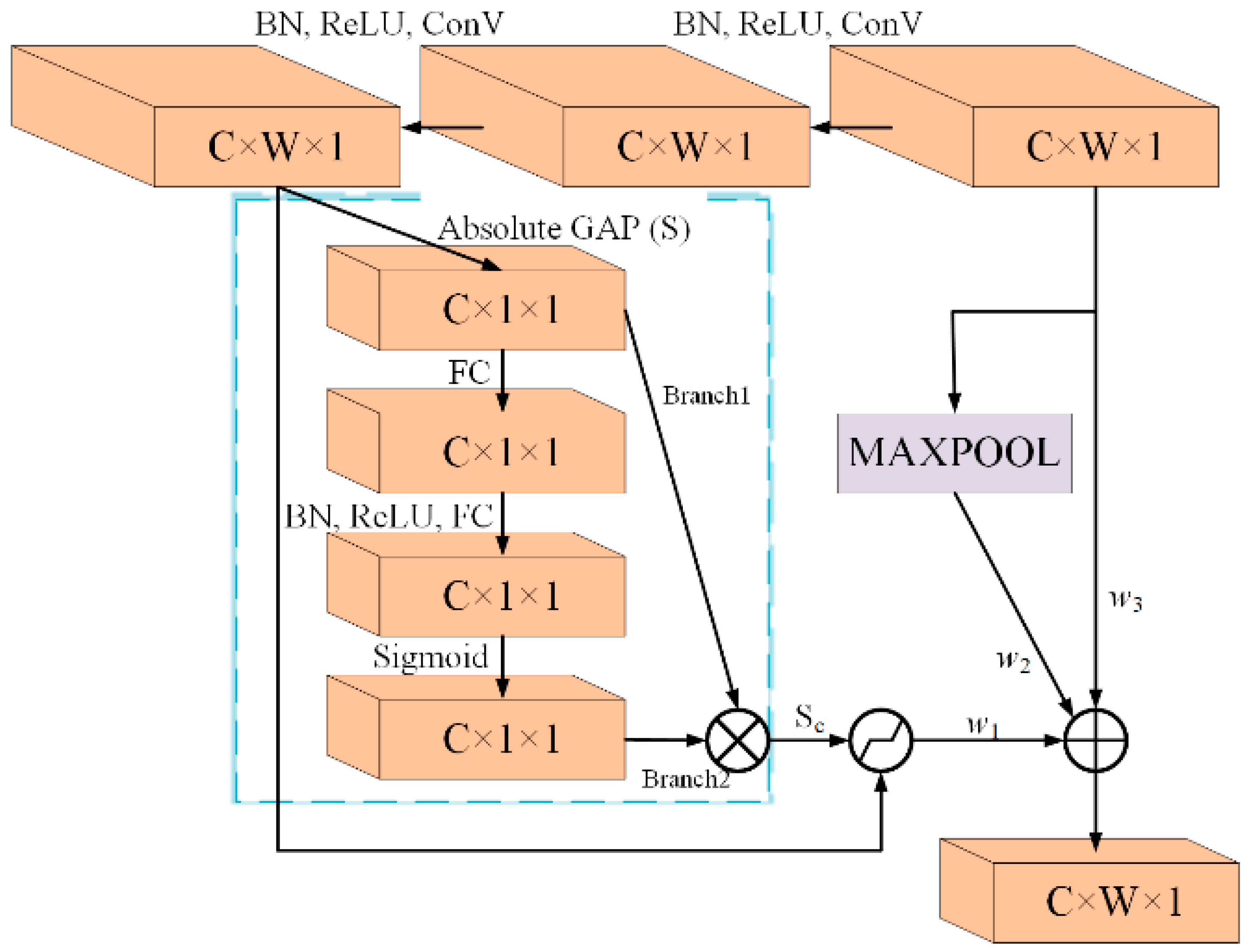
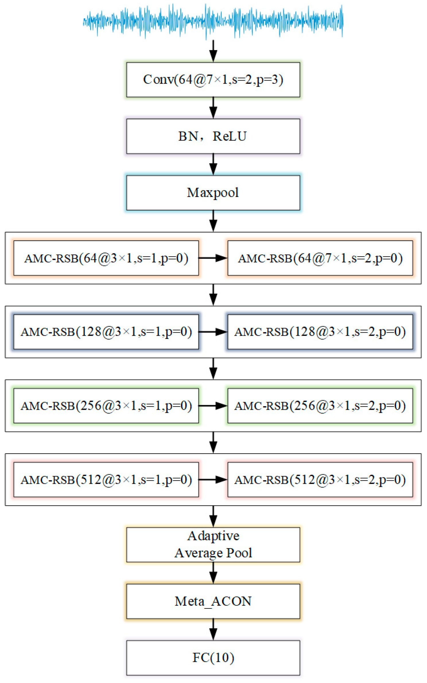
In this paper, we propose an intelligent fault diagnosis method based on AMC-RSN to solve the above problems. Firstly, a channel attention mechanism module is constructed in the residual block and a soft thresholding function is introduced for noise reduction in the original signal. Then, a multi-channel network is constructed to fuse the feature information of each channel to extract as many features as possible. Hereinto, adaptive weights are set in each channel to obtain the most important information, and these weights are updated adaptively as the model is trained to obtain the best values. Finally, the Meta-ACON activation function is used before the fully connected layer to decide whether to activate the neurons by the model outputs, which can improve the classification accuracy of the model. In summary, this paper has three main contributions as follows.
- (1)
A new multi-channel residual network is proposed for extracting richer features in the signal, which solves the problem of insufficient effective feature extraction;
- (2)
An adaptive learning method based on activation function is proposed to activate neurons adaptively, which can effectively avoid the interference of redundant features;
- (3)
In the case of multiple faults in gearboxes, the experimental results show that the proposed method can effectively extract the features of the target faults and classify them accurately.
The remainder of this paper is as follows.
Section 2 presents the theory underlying the AMC-RSN of this paper.
Section 3 presents the principles and architecture of the proposed AMC-RSN. In
Section 4, the validation of the method and the comparison of related models are carried out and the results are discussed.
Section 5 provides a full-text summary.
4. Experimental Validation and Analysis
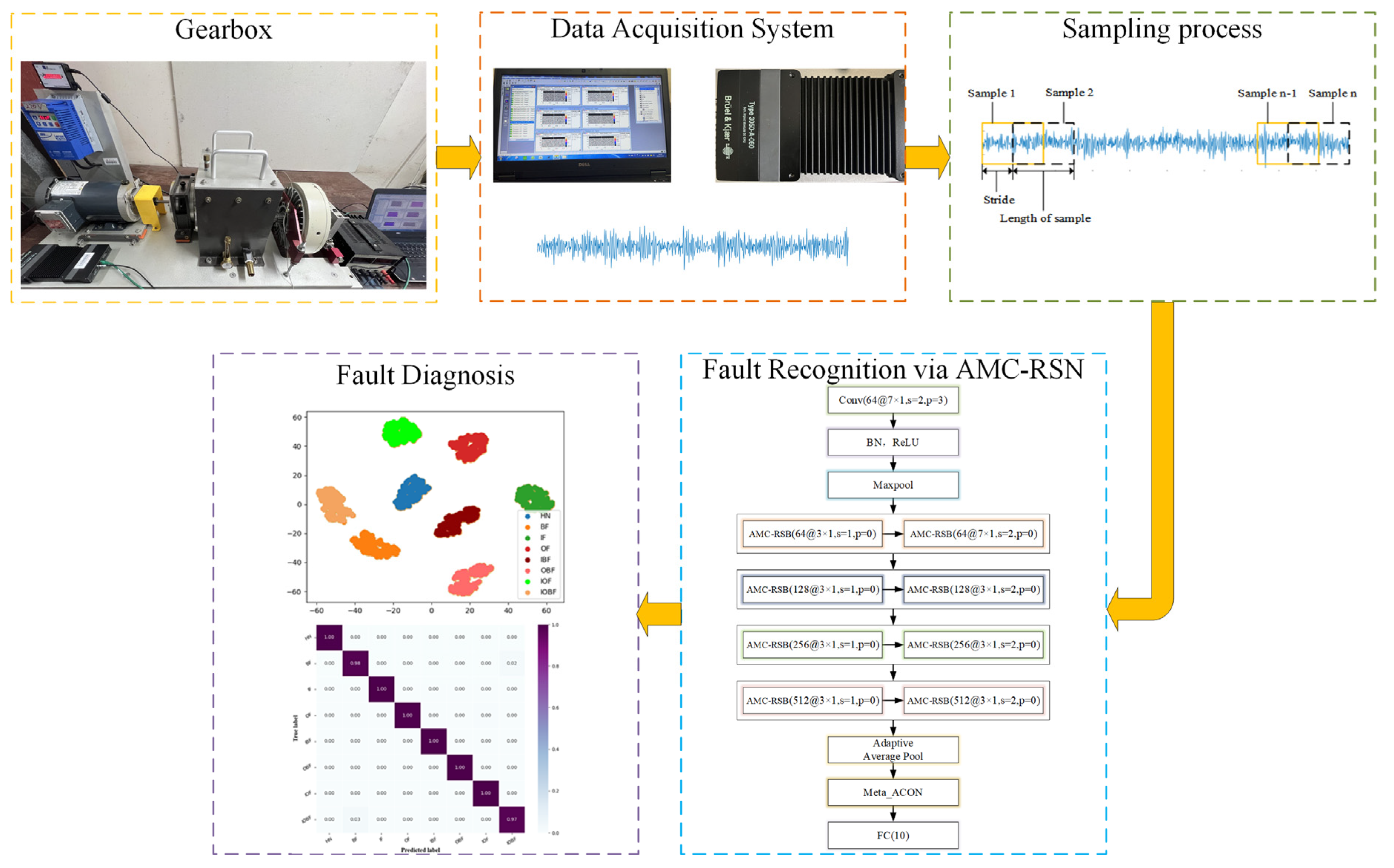
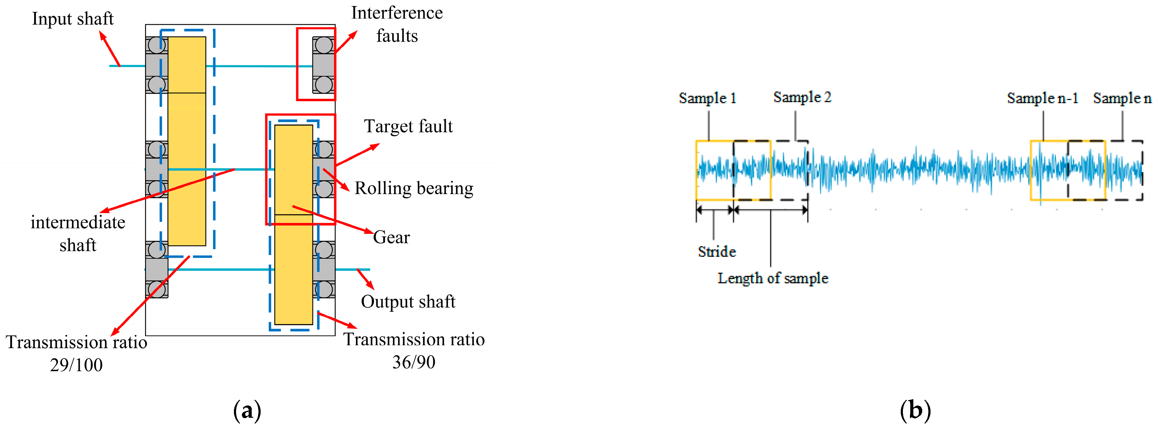
To test the validity of the proposed AMC-RSN, two case studies are conducted in this section. The two different cases used for testing include the rolling bearing and gear datasets. To verify the anti-interference of the proposed AMC-RSN, it is worth noting that the collected vibration signals contain two faulted parts, one of which act as interference item. The experiment setup is shown as
Figure 4a. The parallel gearbox contains two stages of gear reduction, with a primary ratio of 0.29 and a secondary ratio of 0.4. Two cases are conducted to study the effects of the proposed method. In both cases, the right-side rolling bearing of the input shaft is pre-set with ball fault, treated as an interference faulted part. In Case I, different fault types of rolling bearings (gears are healthy) in the intermediate shaft are combined with the above interference faulted part to form the multi-part multi-fault experiment setup. In Case II, different fault types of gears (rolling bearings are healthy) in the intermediate shaft are combined with the above interference faulted part to form the multi-part multi-fault experiment setup. In Case III, different mixed fault types of bearings and gears are set up in the intermediate shaft, and no interference fault is set in the input axis. Due to this setup, along with the noise generated by the machine operation, it will inevitably pose a challenge to the detection and classification of target faults.
To enhance the dataset, all samples are overlapping samples with a sample length of 1024 and a stride of 512, the sampling form is shown in
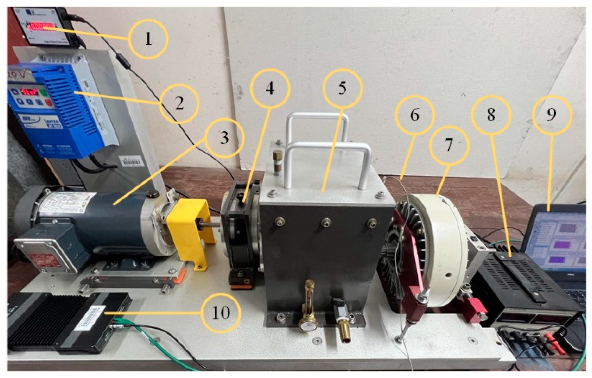
Figure 4b. Vibration data from the different datasets were collected using the SpectraQuest Drivetrain Dynamics Simulator (DDS). The data are collected by the accelerometer, and the arrangement of the sensor is shown in
Figure 5, No. 6. The sampling time is 43.5 s, and the sampling frequency is 12,800 Hz. The length of each fault signal is 556,800, so the number of samples for each fault type after overlapping sampling is 1086. In all experiments, 80% of the training samples and 20% of the test samples are used. The details of the DDS are shown in
Figure 5.
The program uses PyTorch DL software with the Python 3.7 language. The CPU of the computer is configured as Intel Core i7-9750H and the GPU is configured as NVIDIA RTX2060. In the validation session, each test model is the optimal model obtained by 100 epochs of training. To avoid randomness, each method was trained ten times and ten test models were obtained. The Adam optimizer is used to optimize the learning rate during the training process. The loss function is a cross-entropy function.
4.1. Case I
(1) Rolling Bearing Datasets: In the datasets, there are mainly eight fault states, namely health (HN), ball fault (BF), inner ring fault (IF), outer ring fault (OF), inner ring, and ball compound fault (IBF), outer ring and ball compound fault (OBF), inner and outer ring compound fault (IOF), and inner and outer ring and ball compound fault (IOBF). The datasets were collected at a motor speed of 3120 rpm with 2 V (Torque: 4.06 N∙m) load. The datasets of rolling bearing failures for eight different failure types are shown in
Table 1.
(2) Analysis of Fault Diagnosis Results in Rolling Bearing Datasets: To show the superiority of the proposed method, a comparison with other DL methods is conducted in this section. The methods used for comparison contain CNN, deep residual shrinkage network with channel-wise thresholds (DRSN-CW) [
6], multiscale cascade midpoint residual convolutional neural network (MSC-MpResCNN) [
27], and multiscale kernel-based ResCNN (MK-ResCNN) [
26]. To verify the effectiveness of the multi-channel strategy and Meta-ACON, adaptive residual shrinkage network with Meta-ACON activation function (ARSN-M) and adaptive multi-channel residual shrinkage network (AMRS) without Meta-ACON are used for comparison.
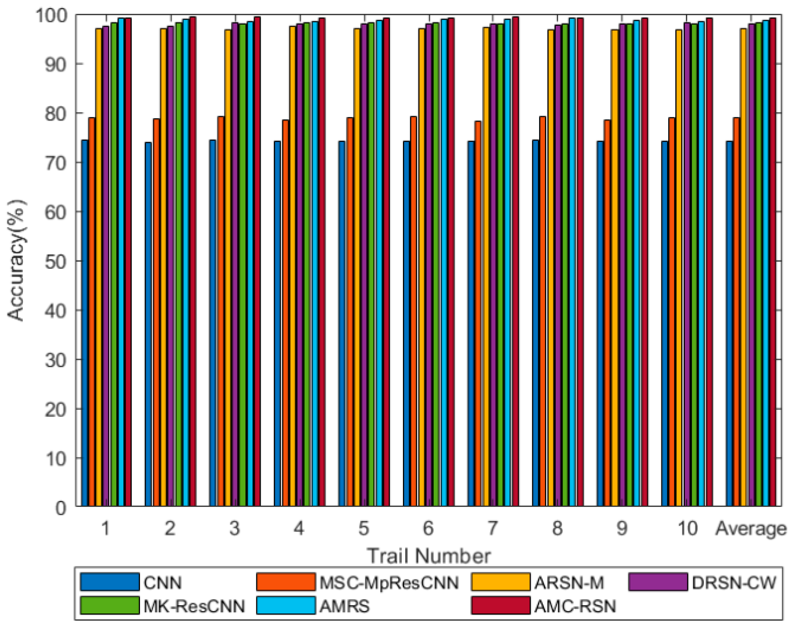
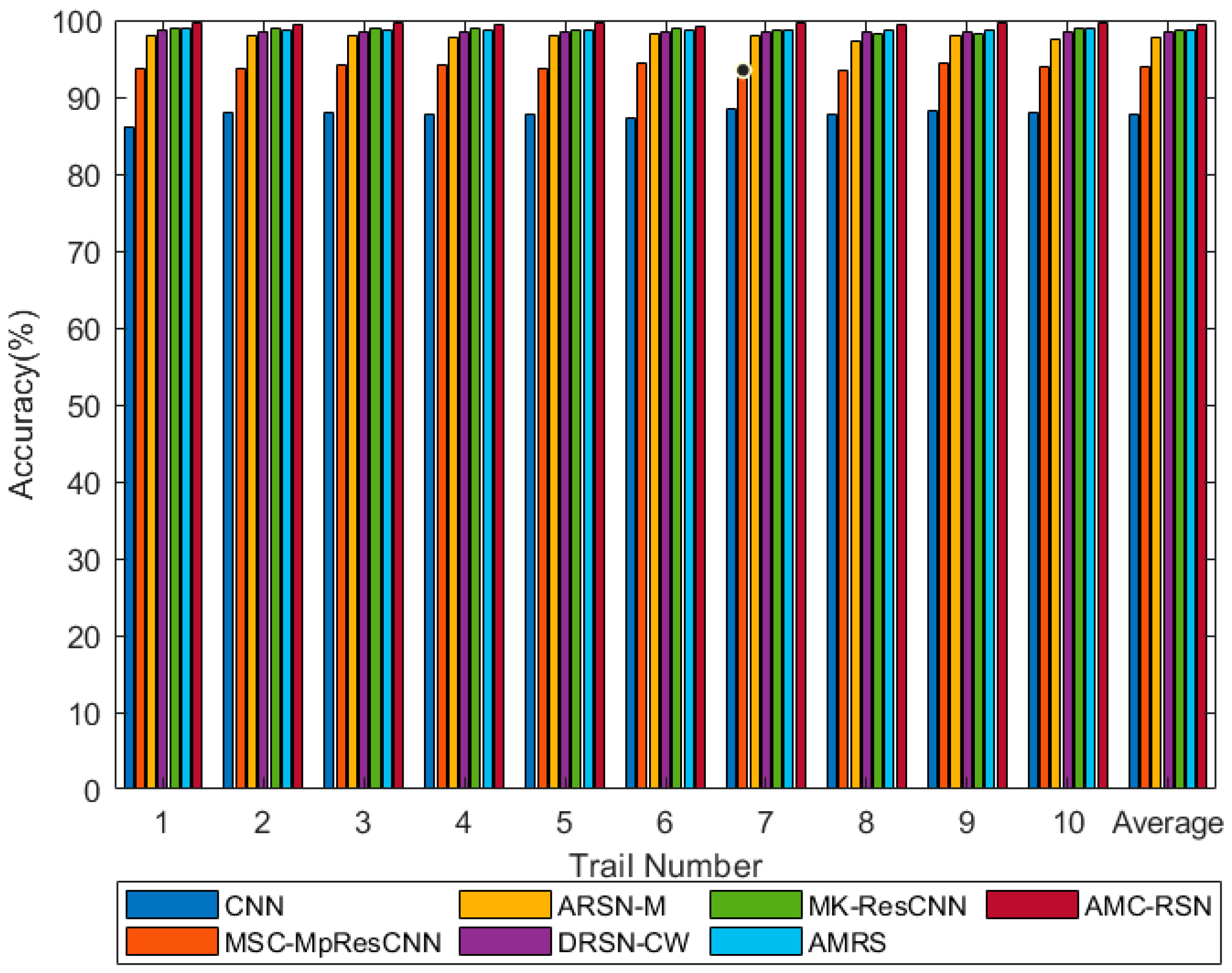
In
Figure 6, we observe that AMC-RSN has the highest classification accuracy in all methods. We can also find that CNN has the worst diagnosis accuracy. Among these different residual networks, AMC-RSN can obtain the best diagnostic results and the highest time consumption. Compared to AMRS and ARSN-M, AMC-RSN can learn the classifier weights adaptively to improve classification accuracy and extract richer features. The tested bearing is shown in
Figure 7. From
Table 2, it is obvious that the average classification diagnosis accuracy of AMC-RSN is the highest, i.e., 99.24%, which is better than the remaining methods. In addition, the proposed method has the smallest standard deviation of 0.11%, which reflect AMC-RSN has robustness.
4.2. Case II
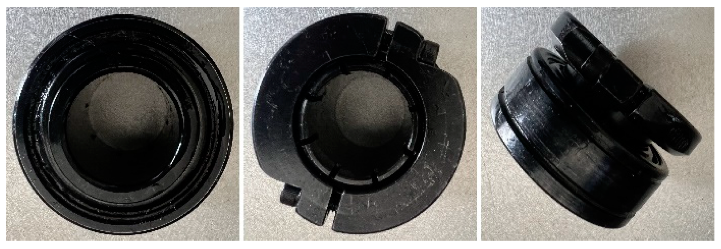
(1) Gear datasets: To further verify the effectiveness of the proposed method, different fault types in the gear datasets are collected and used for validation. As shown in
Figure 8, there are six different damaged types of gears.
As is shown in
Table 3, the gear datasets contain six different fault types, i.e., healthy gear, 1-tooth worn gear, 2-tooth worn gear, 2 mm crack gear, 3 mm crack gear, and 4 mm crack gear. The latter three damages are different crack lengths in the tooth root radial direction. The datasets were collected at a motor speed of 3120 rpm with 2 V (Torque: 4.06 N∙m) load.
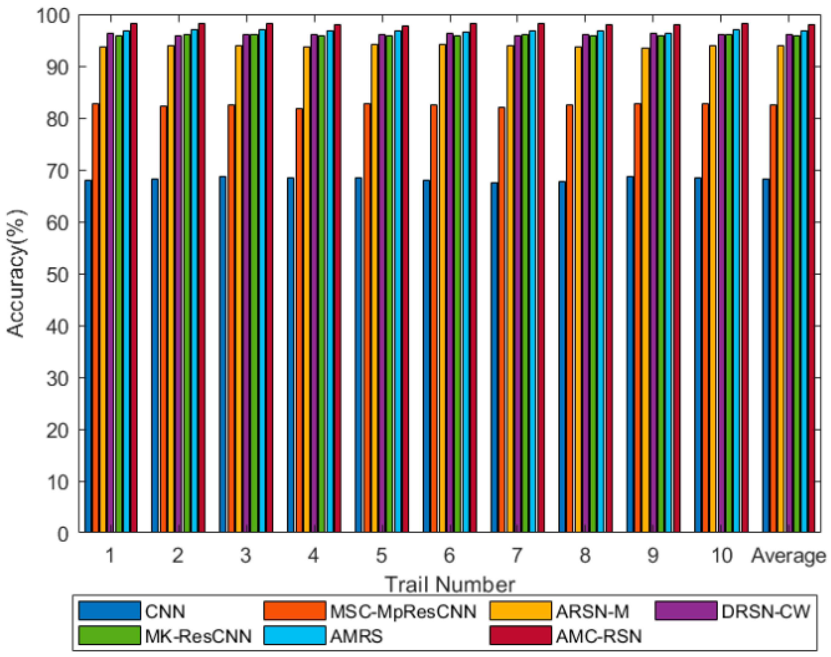
(2) Analysis of Fault Diagnosis Results in Gear Datasets: As is shown in
Figure 9, the proposed AMC-RSN has the best diagnostic effect and the lowest diagnostic accuracy of CNN compared with other methods. From
Table 4, it is noteworthy that the proposed AMC-RSN can obtain the highest accuracy of 98.24% with a standard deviation of 0.16%, which reflects that AMC-RSN has good robustness. Compared with DRSN-CW, MK-ResCNN, and MSC-MpResCNN, the proposed AMC-RSN has significantly improved its ability in extracting the features of the original signal with the highest diagnosis accuracy. Besides, the AMC-RSN has superior performance when compared with the AMRS and ARSN-M.
4.3. Case III
(1) Mixed datasets: In order to further investigate the effectiveness of the proposed method in the diagnosis of mixed gear faults and bearing faults. As shown in
Table 5, the mixed datasets contain six different mixed types of bearing faults and gear faults, including healthy bearing and healthy gear (HH), bearing with inner ring fault and 1-tooth worn gear (IWF), bearing with inner ring fault and 2 mm crack gear (ICF), bearing with outer ring fault and 1-tooth worn gear (OWF), bearing with outer ring fault and 2 mm crack gear (OCF), and bearing with ball fault and 3 mm crack gear (BCF). For consistency with the previous two cases, the datasets were collected at a motor speed of 3120 rpm with 2 V (Torque: 4.06 N∙m) load.
(2) Analysis of Fault Diagnosis Results in Mixed Datasets: As shown in
Figure 10, our proposed AMC-RSN still has better results compared to other methods. From
Table 6, the proposed AMC-RSN can obtain the highest accuracy of 99.49% with the lowest standard deviation of 0.11%, which has better robustness compared to other networks. Compared with AMRS, MK-ResCNN, DRSN-CW, and ARSN-M, the proposed AMC-RSN achieves a slight advantage, while DRSN-CW takes the shortest time. Meanwhile, the CNN and MSC-MpResCNN also achieve higher accuracy rates. Therefore, the fault features of the mixed dataset are more prominent, while the proposed AMC-RSN can learn deeper features and classify them accurately more, which takes relatively more time.
4.4. Visualization Results
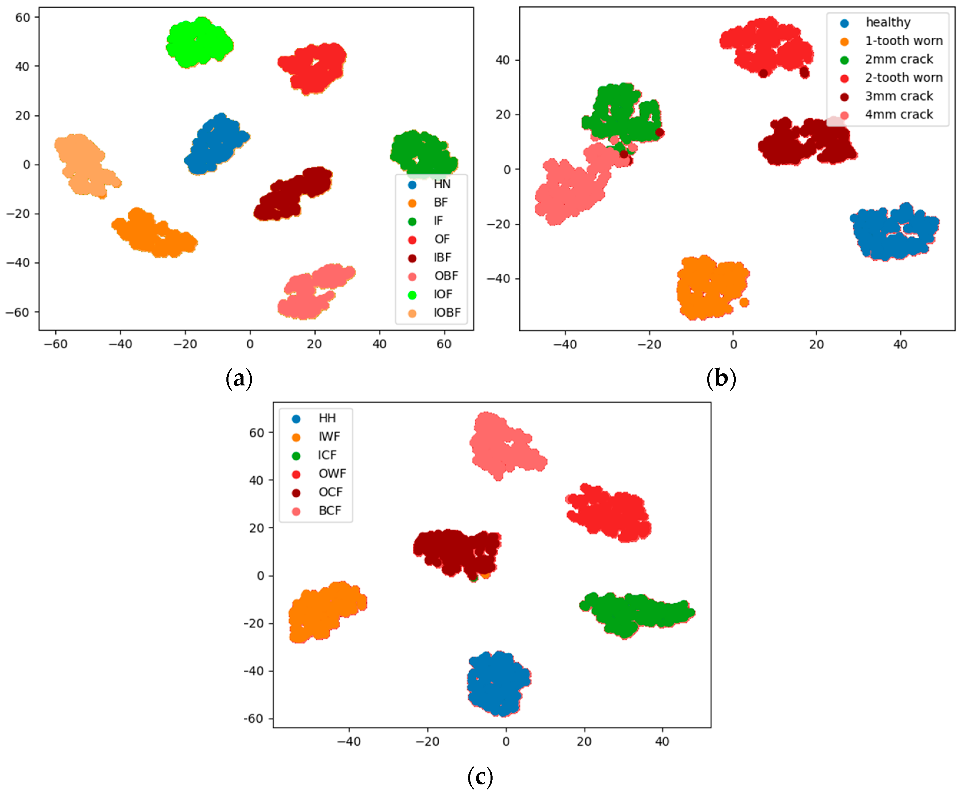
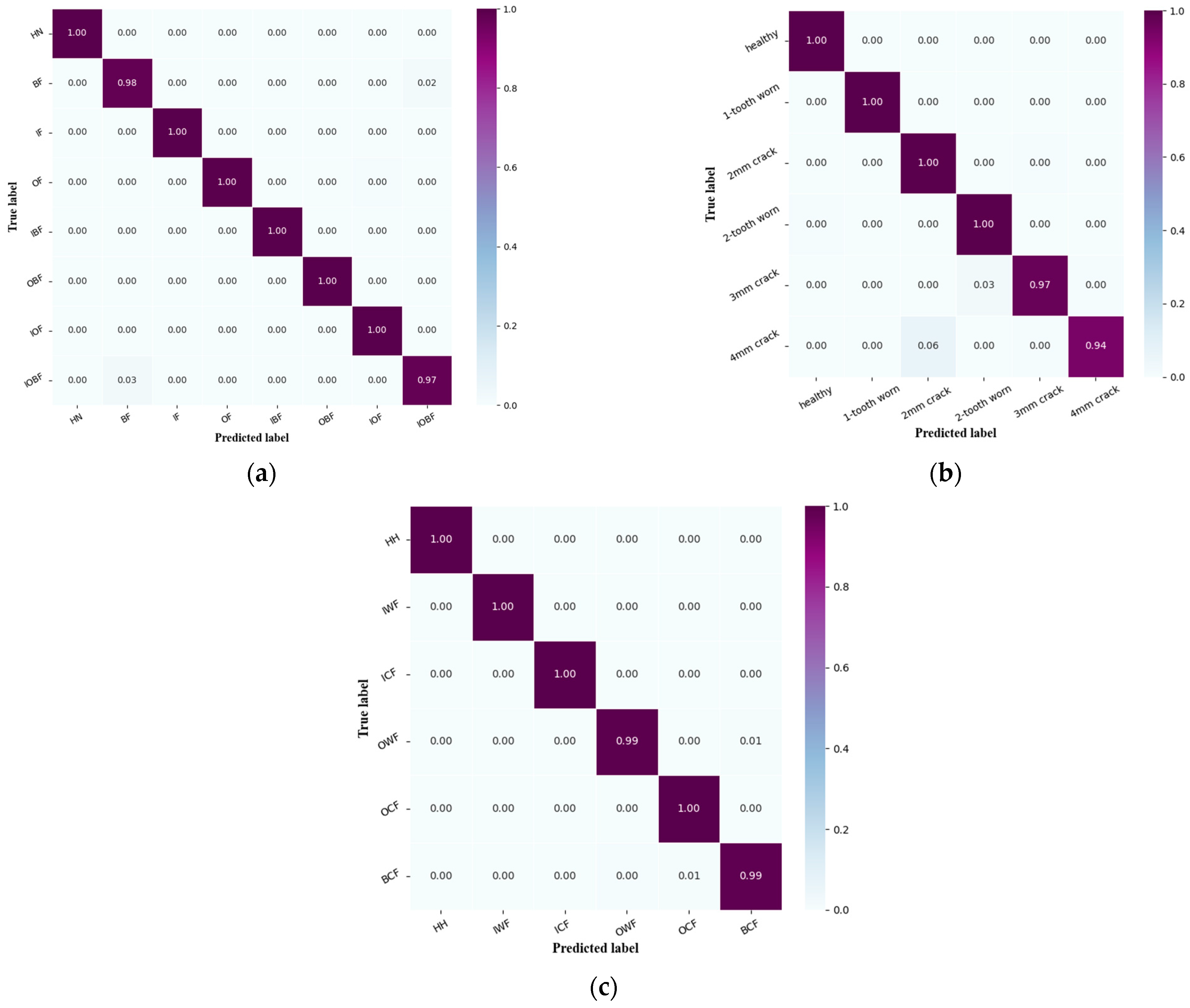
In the test phase, t-SNE and confusion matrix visualization are used to illustrate the best model test results of AMC-RSN in the two cases. In Case I, the feature distribution of the classification results for rolling bearings visualized with t-SNE is shown in
Figure 11a. It can be seen that the inter-class distance is small and the intra-class distance is large for each different type of data sample. Besides, the visualization result of the confusion matrix in
Figure 12a shows that the classification of AMC-RSN is excellent. In Case II, the feature distribution of the classification results for gears visualized with t-SNE is shown in
Figure 11b. The inter-class distances between 4 mm crack and 2 mm crack are relatively small, but other types are relatively large. According to the confusion matrix of gears in
Figure 12b, the overall results are good. So, the different fault types of gear datasets can also be classified by AMC-RSN. In Case III, the feature distribution of the classification results for mixed datasets visualized with t-SNE is shown in
Figure 11c. It can also be seen that the inter-class distance is small and the intra-class distance is large for each different type of data sample. From
Figure 12c, the predicted and true values of the proposed method AMC-RSN are basically consistent.


