Reinforcement Learning for Autonomous Underwater Vehicles via Data-Informed Domain Randomization

Featured Application

The proposed RL via data-informed Domain Randomization (DDR) is designed to stabilize autonomous underwater vehicles and the platforms of underwater vehicle-manipulator systems, which are further subject to unknown dynamics and varying payloads. The approach captures the differences in dynamics between the simulated AUVs and real AUVs, trains the controller in simulations that are suitable for real AUVs, and avoids the tedious procedures of parameter-tuning. The proposed RL-DDR requires only a few training samples, making the controller adaptation efficient for real-time applications.

Abstract

Autonomous Underwater Vehicles (AUVs) or underwater vehicle-manipulator systems often have large model uncertainties from degenerated or damaged thrusters, varying payloads, disturbances from currents, etc. Other constraints, such as input dead zones and saturations, make the feedback controllers difficult to tune online. Model-free Reinforcement Learning (RL) has been applied to control AUVs, but most results were validated through numerical simulations. The trained controllers often perform unsatisfactorily on real AUVs; this is because the distributions of the AUV dynamics in numerical simulations and those of real AUVs are mismatched. This paper presents a model-free RL via Data-informed Domain Randomization (DDR) for controlling AUVs, where the mismatches between the trajectory data from numerical simulations and the real AUV were minimized by adjusting the parameters in the simulated AUVs. The DDR strategy extends the existing adaptive domain randomization technique by aggregating an input network to learn mappings between control signals across domains, enabling the controller to adapt to sudden changes in dynamics. The proposed RL via DDR was tested on the problems of AUV pose regulation through extensive numerical simulations and experiments in a lab tank with an underwater positioning system. These results have demonstrated the effectiveness of RL-DDR for transferring trained controllers to AUVs with different dynamics.

1. Introduction

Autonomous Underwater Vehicles (AUVs) and underwater vehicle-manipulator systems are attracting more attention in marine survey and intervention applications, such as structure inspection, cleaning and repairing, waste searching and salvage, deepwater rescuing, sediment sampling, etc. [1,2,3,4]. However, possible thruster degeneration and damage, various payloads, and disturbances from currents inevitably bring tremendous uncertainties to AUV dynamics models [5]. In addition, other constraints, such as input dead zones and saturations, make it difficult to tune the controller parameters [6]. This paper explores the feasibility of model-free reinforcement learning approaches to these issues in underwater AUV position regulation problems.

Control problems subject to uncertainties have been investigated over the years. For example, the adaptive controller can to model the uncertainties online, and forces the controlled AUV systems to behave as some given reference models [7]. The adaptation is based on current states and errors as inputs, while long-term optimality is often neglected. The backstepping controller can guarantee system stability through its design processes but requires a sufficiently accurate dynamics model [8]. Otherwise, the control gain would be too large for real systems. The controller based on sliding mode requires sufficient time to reach the sliding surface and provide robustness [9]. These above-mentioned approaches may have provable stabilities without considering the dead zones and saturations of the control inputs.

To be applicable to dynamical systems with input saturations, many existing control approaches assume that the model mismatch is small. Then, these controllers have sufficient margins to suppress uncertainties and input constraints, offering stability to the controlled AUV systems. When applied to real systems, the controller parameters have to be re-tuned according to the altered dynamical system. More importantly, the assumption of small differences in dynamics models may not hold for shallow-water AUVs. In underwater applications, water weeds may tangle one or more thrusters, limiting their maximal thrusts, and the AUVs may be subject to various payloads. All these factors make the model uncertainties quite large.

Controllers based on deep learning have been studied in [10]. Classical model-free RL can overcome the above-mentioned issues of uncertainties, but often relies on a large number of samples to train controllers from scratch. Millions of interactions between the controller and the targeted system are time-consuming and may damage the system itself. Therefore, it is preferable to train a controller in a simulated system and then apply it to a real AUV system. However, the trained controllers often perform unsatisfactorily on real AUVs. This is because the distributions of the state and AUV dynamics in numerical simulations do not match those of real AUVs. Much effort has been devoted to transferring the controller to a different system, referred to as transfer RL [11]. In the context of transfer RL, the trained controller is obtained offline from a source domain with source dynamics. The trained controller is referred to as the source controller. Then, the source controller is transferred to a target controller and is applied to a target system in an online target domain, where the target system is often unknown.

The idea of transferring controllers to a different system has been explored in manipulator control [12]. Recently, a model-free transfer RL on AUV control was validated on numerically simulated AUVs [13]. In the transfer reinforcement learning of robot control, the source domain and source dynamics are often numerically simulated, while the target domain and the target dynamics pertain to the real systems [14]. The source controller is trained for the source dynamics in the source domain and transferred to obtain the target controller to control the target dynamical system in the target domain. In another type of transfer reinforcement learning, the source domain and target domain may share the same dynamics model and state spaces but differ in the definitions of objective functions [15], which is not discussed in this paper.

The correlation across domains is key to transferring the source controller to the target domain [16]. Domain-invariant essential features and structures were studied to build and transfer the controller across domains [17]. The correspondence between domains can be found by analyzing the unpaired trajectories between two different domains [18].

Another issue for sim-to-real transfer RL is robustness. Domain randomization algorithms vary the parameters of the numerically simulated dynamics models and obtain a controller through RL [19]. RL based on domain randomization [20] is a popular technique to reduce domain and dynamics mismatches. Instead of directly adding Gaussian noise to the outputs of the simulated dynamics models, the noise is added to the parameters of dynamics models, allowing for more diverse distributions that can cover the actual distributions of the AUV states and dynamics. The trained controller is robust to the simulated dynamics, which has a high probability of covering the actual manipulator states and dynamics. Therefore, the trained controller has better robustness than classical RL. This approach has been successful in the control of manipulators, where an accurate dynamics model is required and a friction model is considered [20].

It is preferable to adjust the parameter noise in the domain randomization according to the actual data. The adaptive domain randomization approach adjusts the weight of parameter particles to narrow the gap between simulators and real AUV dynamics [21]. However, the effectiveness of such a strategy is based on an accurate parametric dynamics model. This assumption may not be suitable for AUVs. Existing AUV models have more unmodeled dynamics, which are difficult to describe in the simulations via domain randomization techniques. Therefore, it is desirable to quickly modify the simulator to behave as a real AUV through a data-driven module. Still, the process of obtaining a data-enabled module to close the gap between source dynamics and target dynamics may take a tremendous amount of time. Therefore, it is better if only a few samples of the real AUVs are required to quickly adapt the source controller.

State-of-the-art algorithms based on feedback control may not be able to deal with dynamics that are suffering significant changes, such as shifts in control channels or thruster failures. These changes in dynamics may occur online and jeopardize the AUV system if the same controller is used. On other hand, reinforcement learning approaches require extensive interactions between controllers and the targeted AUV and may adapt themselves to the new dynamics. This paper proposes a transfer RL approach via data-informed domain randomization (DDR) to efficiently adapt the source controller. The contributions are as follows.

(i)

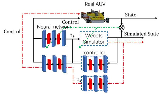
Data-informed domain randomization. In this paper, the numerical dynamics model (the source model) is built on a Webots simulator. According to the collected data of a real AUV, the control inputs and state outputs regarding the source model are quite different from those of the target model. A neural network is aggregated onto the Webots source model and is quickly adapted online to match the difference between the source model and the target model, reducing the gap between the source and target dynamics.

(ii)

Controller adaptation mechanism. Based on the matching from the proposed DDR, the correlation between the source and target controllers is used to quickly align the source control signals to the target ones. Since the source task and domain task only differ in dynamics models, the mismatch is captured by a small neural network that can be retrained in less than a second with newly collected data.

(iii)

Validation through numerical simulations and tank experiments. The proposed RL via DDR was validated by numerical simulations of AUVs with manually designed and mismatched dynamics models: these have different thruster configurations and capabilities. RL via DDR was also tested in a sim-to-real transfer setting, where the transferred controller was tested for an AUV in a tank and the parameters of the AUV were varied.

The remainder of this paper has the following structure. The position regulation problem of an AUV and the transfer RL problem are introduced in Section 2. Section 3 outlines the algorithm of classical RL, followed by the DDR approach, and RL via DDR in Section 4. Section 5 summarizes the simulation results of transfer RL on the AUVs in the Webots simulator and results on sim-to-real experiments. At last, the discussion and conclusions are given in Section 6.

2. Problem Formulation

This paper studies the pose regulation problem of the AUV subject to model uncertainties and other input constraints, such as dead zones and input saturations. Let $X_i{Y}_i{Z}_i$ denote the earth-fixed reference frame and $X_b{Y}_b{Z}_b$ denote the body-fixed reference frame [1], as shown in Figure 1. Axis $O_i{X}_i$ and Axis $O_i{Y}_i$ are in the horizontal plane, Axis $O_i{Z}_i$ is the gravity direction. The body-fixed frame $X_b{Y}_b{Z}_b$ is attached to the AUV center and the $O_b{X}_b$ axis coincides with the AUV heading. The $O_b{Y}_b$ axis is along the starboard direction. The AUV pose in the frame $Z_i{Y}_i{Z}_i$ is defined as its position ${[x_i,y_t,z_i]}^T$ and attitude ${[\rho ,\psi ,\theta ]}^T$. Similar to many AUVs, the restoring force is often sufficiently large to maintain its roll $\rho$ and pitch $\psi$ close to zero under all circumstances. The restoring force can be manually designed by adjusting the distance between the mass center and the buoyancy center of the AUV.

As a result, in this paper, the studied AUV is described by motions of four Degrees Of Freedom (DOFs), including the linear motions along the $O_b{X}_b$, $O_b{Y}_b$, and $O_b{Z}_b$ directions and the yaw motion around the $O_b{Z}_b$ axis. Then, the AUV state pose $\mathbf{\eta }$ with respect to the earth-fixed frame $Z_i{Y}_i{Z}_i$ is redefined as

$${\mathbf{\eta }}_i\triangleq {[x_i,y_i,z_i,{\theta }_i]}^T,$$

where $x_i$, $y_i$, and $z_i$ are the AUV’s position, and ${\theta }_i$ denotes the AUV’s heading in the earth-fixed frame. Then, the AUV’s velocity ${\mathbf{\nu }}_i$ in $X_i{Y}_i{Z}_i$ is defined as

$${\mathbf{\nu }}_i\triangleq {\dot{\mathbf{\eta }}}_i={[u_i,v_i,w_i,{\omega }_i]}^T,$$

where $u_i$, $v_i$, and $w_i$ are translational velocities in the x-, y-, and z-axes in the inertial frame, and ${\omega }_i$ is the angular velocity along the z-axis in the inertial frame. Then, the generalized velocity in $X_b{Y}_b{Z}_b$ is given as

$$\mathbf{\nu }={[u_b,v_b,w_b,{\omega }_b]}^T,$$

where

$${[u_b,v_b,w_b]}^T=\mathbf{R}\left({\theta }_i\right){[u_i,v_i,w_i]}^T,$$

$${\omega }_b={\omega }_i,$$

and $\mathbf{R}(\theta +i)$ denotes the transform from Frame $X_i{Y}_i{Z}_i$ to Frame $X_b{Y}_b{Z}_b$. Let the generalized control $\mathbf{\tau }$ from lumped thrusts in Frame $X_b{Y}_b{Z}_b$ be denoted as $\mathbf{\tau }\triangleq {[{\mathbf{\tau }}_x,{\mathbf{\tau }}_y,{\mathbf{\tau }}_z,T_z]}^T$, which may not act through the center of mass. In fact, the mapping between thrusts to the generalized control $\mathbf{\tau }$ may not be accurately known, due to manufacturing issues.

The dynamics model of the AUV is often described in the body frame [22] as

$$\mathit{M}\dot{\mathbf{\nu }}+\mathit{C}\left(\mathbf{\nu }\right)\mathbf{\nu }+\mathit{D}\left(\mathbf{\nu }\right)\mathbf{\nu }+\mathit{g}\left(\mathbf{\eta }\right)=\mathbf{\tau },$$

(1)

where $\mathit{M}$ denotes the inertia matrix with added mass from motion in the water, $\mathit{D}$ denotes the coefficient matrix of the drag forces, $\mathit{C}$ denotes the Coriolis matrix, and $\mathit{g}$ is the lumped vector of gravity and buoyancy. The value of $\mathit{g}$ can be assumed to be constant, while the values of other matrices are partially determined by the velocities of the AUV and water current, and are, therefore, difficult to estimate. The dynamics model in Equation (1) only captures the main aspects of the actual system under mild conditions, leaving some effects unmodeled, such as thruster dynamics. The control inputs $\mathbf{\tau }$ are subject to constraints from the phenomena of saturations and dead zones, which are, respectively, given by

$$\begin{array}{c}\hfill \underline{\mathbf{\tau }}\le \mathbf{\tau }\le \overline{\mathbf{\tau }}\\ \hfill \left|\mathbf{\tau }\right|\ge {\mathbf{\tau }}_d,\end{array}$$

(2)

where $\underline{\mathbf{\tau }}$ and $\overline{\mathbf{\tau }}$ denote the saturation bounds of the control inputs, $|·|$ denotes the absolute operation, and ${\mathbf{\tau }}_d$ denotes the dead band. Let $\mathcal{U}$ denote the set of control that satisfies Equation (2). However, the feasible set $\mathcal{U}$ may not be accurately estimated due to varying power supply and current conditions.

Problem 1 

(Position Regularation Problem). Design a controller that can bring the AUV starting at ${\mathbf{\eta }}_i\left(0\right)$ to the origin ${\mathit{O}}_i$, subject unknown dynamics model (1), and the constraints of the dead zones and saturations (2).

This paper explores the feasibility of RL techniques to train a controller from numerical simulations built on Equation (1). The continuous-time model in (1) is converted into a discrete-time model by Taylor’s first-order expansion, as shown below:

$$\mathbf{\nu }(t+1)=\mathbf{\nu }\left(t\right)+{\mathit{M}}^{-1}\mathbf{\tau }\left(t\right)\Delta t-{\mathit{M}}^{-1}\zeta (\mathbf{\nu }\left(t\right),\mathbf{\eta }\left(t\right))\Delta t,$$

(3)

where

$$\zeta \left(\mathbf{\nu }\right(t),\mathbf{\eta }(t\left)\right)=\mathit{C}\left(\mathbf{\nu }\right(t\left)\right)\mathbf{\nu }\left(t\right)+\mathit{D}\left(\mathbf{\nu }\right(t\left)\right)\mathbf{\nu }\left(t\right)+\mathit{g}\left(\mathbf{\eta }\right(t\left)\right)$$

(4)

and $\Delta t$ is the sampling time. The forward dynamics model in (3) is denoted as ${\mathcal{F}}_s$.

This model can be simulated with estimates of unknown parameters by the Webots simulator and the controller can be trained to solve Problem 1 of the simulated system (3). The controller ${\mathit{u}}_s$ outputs the control vector $\mathbf{\tau }\left(t\right)$ at time t, i.e.,

$$\mathbf{\tau }\left(t\right)=\mathit{u}\left[\mathbf{\nu }\right(t),\mathit{e}(t\left)\right],$$

where ${\mathit{e}}^T\left(t\right)$ is the error of position regulation viewed in the body frame and is obtained by

$${[{\mathit{e}}^T\left(t\right),1]}^T\triangleq {\mathit{T}}^T\left({\mathbf{\eta }}_i\right){[{\mathbf{\eta }}_i^T,1]}^T.$$

The transformation matrix $\mathit{T}\left({\mathbf{\eta }}_i\right)$ transforms a point in the body frame to the earth-fixed frame. The controller $\mathit{u}(·)$ maps from the AUV velocity and position errors to control inputs. Let $\mathbf{y}\left(t\right)\triangleq {[{\mathbf{\nu }}^T\left(t\right),{\mathit{e}}^T\left(t\right)]}^T$ and refer $\mathbf{x}\left(t\right)$ as the AUV state at time t. It is assumed that the AUV state can be acquired with small noises at high frequencies.

The controller trained in the source domain ${\mathcal{D}}_s$ under the source dynamics models ${\mathcal{F}}_s$ (see Equation (3)) is denoted as ${\mathit{u}}_s$, referred to as the source controller. The source controller would be applied to a target dynamical system ${\mathcal{F}}_t$ in a target domain ${\mathcal{D}}_t$. The forward dynamics model ${\mathcal{F}}_t$ presents a real AUV system or a simulated AUV with a different dynamics model. Since the direct application of ${\mathit{u}}_s$ on ${\mathcal{F}}_t$ brings unsatisfactory results, ${\mathit{u}}_s$ has to be transferred to obtain ${\mathit{u}}_t$ for better performance.

Problem 2 

(Controller Transfer Problem). Design an approach to learn a source controller ${\mathit{u}}_s$ for the source dynamics ${\mathcal{F}}_s$ and to transfer ${\mathit{u}}_s$ to the target dynamical system ${\mathcal{F}}_t$ and obtain a target controller ${\mathit{u}}_t$, such that the Problem 1 of the target system ${\mathcal{F}}_t$ can be solved by ${\mathit{u}}_t$.

Model-free RL can deal with uncertainties and train controllers on deterministic dynamical systems with various parameters to improve the stability of the trained controller ${\mathit{u}}_s$ the. However, dynamics models from through-parameter randomization may not cover those in the target domain. To this end, in this paper, a data-informed domain randomization approach is developed to solve Problem 2. In the meantime, the model mismatches between the source and target dynamics models have to be quickly estimated online to efficiently adjust the controller ${\mathit{u}}_t$.

3. Reinforcement Learning

This section briefly describes the RL approach to solve Problem 1 of the simulated AUV. As shown in Figure 2, the learning procedure interacts with the simulator and collects the trajectories and rewards. The task in Problem 1 is converted to an optimization problem as

$$\begin{array}{c}\hfill maxJ=\sum _{t=1}^{\infty }{\gamma }^{t}r\left(t\right),\end{array}$$

(5)

where $\gamma$ is a discount factor that penalizes long-term rewards and the reward function R is defined as follows.

$$r(\mathit{e},\mathit{v},\mathbf{\tau })\triangleq -{{\alpha }_1}^T\Vert \mathit{e}\Vert -{{\alpha }_2}^T\Vert \mathbf{\nu }\Vert -{{\alpha }_3}^T\Vert \mathbf{\tau }\Vert ,$$

(6)

where $\Vert ·\Vert$ denotes $L2$-norm. The term $\mathit{e}\in {\mathbb{R}}^3$ is the regulation error on positions, $\mathit{v}\in {\mathbb{R}}^4$ is the AUV’s generalized velocity and it has to be zero when the AUV is at the origin in Frame $X_i{Y}_i{Z}_i$, and $\mathbf{\tau }\in R^4$ denotes the control inputs. The weights ${\mathbf{\alpha }}_1$, ${\mathbf{\alpha }}_2$, and ${\mathbf{\alpha }}_3$ are positive parameters and are defined by users. In this paper, they were chosen such that ${\mathbf{\alpha }}_1\gg {\mathbf{\alpha }}_2\gg {\mathbf{\alpha }}_3>0$. The reward function has to be designed or learned to reflect the control perpurse, which is a hot topic as it affects the convergence process in the learning and stability performance of the AUV [23].

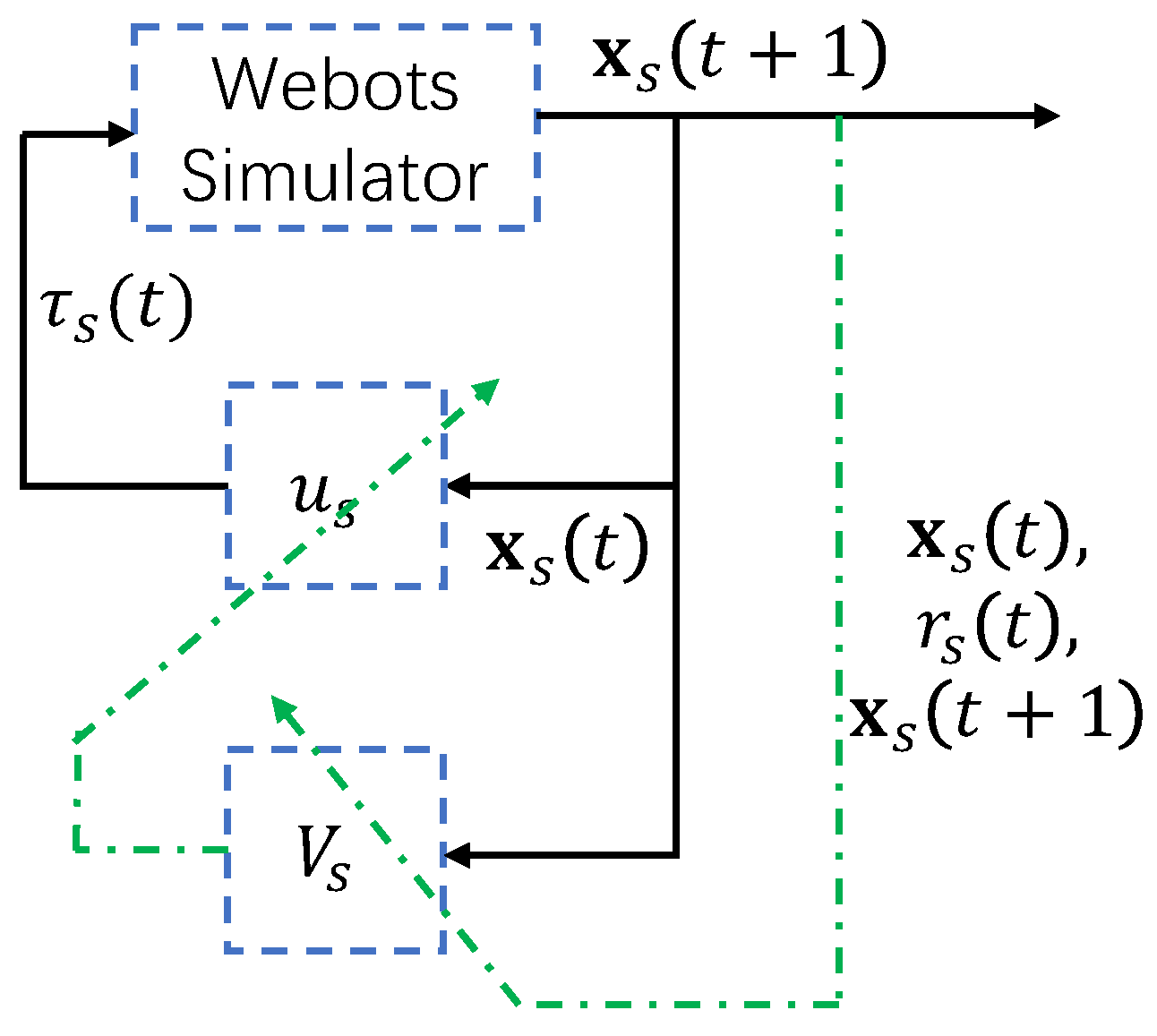
The optimization of the objective (5) is solved against the equality constraints from the AUV dynamics model (3) and the inequality constraints from the control dead zones and saturations (2), outputting the source controller ${\mathit{u}}_s$. These two types of constraints are simulated in the Webots simulator and are rediscovered by the interaction between RL and the simulator by the data ${\{{\mathit{x}}_s\left(t\right),{\mathbf{\tau }}_s\left(t\right),{\mathit{x}}_s(t+1),r_s\left(t\right)\}}_{t\in I_t}$, where $I_t$ is the index set.

RL is essentially a exploration-and-exploitation algorithm that updates its controller through interactions between the learning agent and the simulator (i.e., $\{{\mathit{x}}_s\left(t\right),{\mathbf{\tau }}_s\left(t\right),$${\mathit{x}}_s(t+1),r_s{\left(t\right)\}}_{t\in I_t}$). After being fitted in Markovian decision processes, the objective function is the cumulated rewards and should be maximized. The reward function is defined in Equation (5) [24]. In the tth iteration, the control inputs $\mathbf{\tau }\left(t\right)\in \mathcal{U}$ are chosen by the controller ${\mathit{u}}_s$ based on the state ${\mathit{x}}_s\left(t\right)$ (i.e., the current regulation error ${\mathit{e}}_t$ and velocities ${\mathit{nu}}_t$). The simulator receives the control inputs $\mathbf{\tau }\left(t\right)$ and outputs the AUV state ${\mathit{x}}_s\left(t\right)$ after a one-step simulation and a reward value defined in Equation (6). The obtained data ${\{{\mathit{x}}_s\left(t\right),{\mathbf{\tau }}_s\left(t\right),{\mathit{x}}_s(t+1),r_s\left(t\right)\}}_{t\in I_t}$ are used to update the controller network ${\mathit{u}}_s$ and the critic network $V_s$, as shown in Figure 2. The critic $V_s$ is essentially the objective function evaluated at the state ${\mathit{x}}_s$, conditioned on the controller ${\mathit{u}}_s$, which is not optimal before the convergence of the learning process. The controller ${\mathit{u}}_s$ is then updated by maximizing the critic $V_s$ at given ${\mathit{x}}_s$. The procedures are briefly outlined in Algorithm 1.

While there are many methods to train the controller network, this paper adopts the Soft Actor-Critic (SAC) [25], which is an open-source off-policy learning algorithm. As reported by many researchers, SAC can achieve sufficient results in benchmark problems.

Algorithm 1: Learning Source Controller Network

4. Transfer RL via Data-Informed Domain Randomization

In the studied transfer learning of Problem 2, the state space and the control space between the source domain and the target domain share the same dimensions. This section explores a method to train a mapping $H({\mathit{x}}_s,{\mathbf{\tau }}_s)$ that transfers ${\mathit{u}}_s$ to obtain ${\mathit{u}}_t$ to match the difference between the source dynamics and target dynamics. In addition, it is required that the training of $H({\mathit{x}}_s,{\mathbf{\tau }}_s)$ relies on a limited number of data, which can be collected within a few minutes of collection on the real AUV. This section introduces a data-informed domain randomization approach.

4.1. Data-Informed Domain Randomization

Instead of directly adding Gaussian noise to the outputs of the simulated dynamics models, the noise is added to the parameters of dynamics models, allowing for more diverse distributions that can cover the actual distributions of the AUV states and dynamics. In each training episode, the parameters in the AUV dynamics model (3) include the inertia matrix $\mathit{M}\in \mathcal{M}$, the drag matrix $\mathit{D}\in \mathcal{D}$, the Coriolis matrix $\mathit{C}\in \mathcal{C}$, the vector $\mathit{g}\in \mathcal{G}$ of lumped gravity and buoyancy. The sets $\mathcal{M}$, $\mathcal{D}$, $\mathcal{C}$, and $\mathcal{G}$ of these parameters can be estimated [1]. The parameters are randomly sampled from $\mathcal{M}$, $\mathcal{D}$, $\mathcal{C}$, and $\mathcal{G}$. Besides, there are uncertainties regarding the transform matrix from thruster forces to the generalized force that acts through the AUV’s center of mass. These uncertainties are also added to the Webots simulator. The control inputs $\mathit{tau}$ are subject to constraints from the phenomena of saturations and dead zones, which are determined by $\underline{\mathbf{\tau }}$ and $\overline{\mathbf{\tau }}$ and ${\mathbf{\tau }}_d$, respectively. These constraints are also randomly chosen according to an estimated set.

As illustrated in Figure 3, following the above-mentioned domain randomization approach, the dashed ellipse denotes the set ${\mathcal{F}}_s$ of the AUV dynamics models that can be simulated in Webots. The solid ellipse presents the set ${\mathcal{F}}_t$ of the real AUV under various conditions, such as thruster configurations and payloads. It is highly possible that the dashed ellipse and the solid ellipse only share a few common dynamics. Therefore, it is difficult to guarantee the stability of the AUV if the trained source controller ${\mathit{u}}_s$ is directly applied to the real AUV. ${\mathit{u}}_s$ might only be robust to the variations in the AUV dynamics in ${\mathcal{F}}_s\cap {\mathcal{F}}_t$.

However, this method is only applicable to the case where the set ${\mathcal{F}}_t$ of target dynamics (the solid ellipse) is contained by the set ${\mathcal{F}}_t$ of source dynamics (the dashed ellipse), as shown in Figure 4a. In this case, the trained controller ${\mathit{u}}_s$ is robust to the dynamics in the solid ellipse. The obtained controller ${\mathit{u}}_s$ maximizes the expectation of the objective function (5) over all possible dynamics in ${\mathcal{F}}_s$. In other words, the expectation of the objective function (5) is not optimized over all possible dynamics in ${\mathcal{F}}_t$. One way to reduce this gap is to adjust the parameter distribution so that ${\mathcal{F}}_s$ is close to ${\mathcal{F}}_t$.

Many adaptive domain adaptation techniques have been studied, and they bias the distribution of parameters based on the trajectory data collected from the target domain ${\mathcal{D}}_s$. The likelihood of the trajectory obtained from various simulated dynamics compared to an obtained trajectory from the real AUV can be computed and used to update the weights of the parameter particles. In each episode, particles with different weights are used to sample parameter values following the particle filter strategy, and to train the source controller ${\mathit{u}}_s$. This procedure identifies the system parameters and many other similar approaches can be explored in the future.

However, the performance of the above strategy heavily relies on the assumption that ${\mathcal{F}}_t\subset {\mathcal{F}}_s$. While treating unmodelled dynamics as noise, the nominal behavior of the actual AUV dynamics is contained by the set of source dynamics models. The actual system may exhibit dynamics that are not covered by ${\mathcal{F}}_s$. Therefore, this paper proposes the following data-informed domain randomization (DDR) approach, as shown in Figure 5. It is based on the assumption that the variation in a given dynamics model can be covered by the mapping between the control inputs. The mapping G is illustrated as the “G” block of the diagram in Figure 5.

The mapping has a limited number of neurons, only requires a few training samples and can deal with many changes regarding the real AUV—for example, when one truster is tangled by seaweeds and its thruster force is degenerated. In other cases, when the external force from payloads changes, the mapping of the forces can also implicitly estimate the payloads. The scale between inputs forces and mass and other terms can also be captured by the mapping G. The mapping between controllers ${\mathit{u}}_s$ and ${\mathit{u}}_t$ is then defined as

$$\begin{array}{c}\hfill {\mathbf{\tau }}_s=G\left({\mathbf{\tau }}_t\right).\end{array}$$

(7)

The goal of the DDR is to reduce the gap between the outputs from the simulated dynamics model and the trajectories collected from the actual AUV. The loss function in training is given as $\Vert {\mathcal{T}}_s-{\mathcal{T}}_t\Vert$, where the trajectory ${\mathcal{T}}_t$ is collected from the actual AUV, while ${\mathcal{T}}_s$ is obtained from the numerical simulation. Since it might be difficult to find a close enough trajectory, it is better to create an inverse dynamics model of the simulated model (3). Therefore, in this paper, an inverse model of (3) was obtained via supervised training. The obtained inverse dynamics model is denoted as $R\left(\mathbf{\nu }\right(t),\mathbf{\nu }(t+1),\mathbf{\eta })$.

In online applications, the adaptive domain randomization approach aims to reduce the variance in parameters. When trajectories are obtained from the real AUV, control signals are also obtained. From the inverse model, the control inputs can be calculated from Equation (7). The loss function to train G is given as

$$\begin{array}{c}\hfill \mathcal{L}\left(G\right)\triangleq \Vert R(\mathbf{\nu }\left(t\right),\mathbf{\nu }(t+1),\mathbf{\eta })-G\left({\mathbf{\tau }}_t\right)\Vert \end{array}$$

(8)

Through learning G, this approach is able to quickly capture the changes in the dynamics model of the real AUV. The obtained mapping $G\left({\mathbf{\tau }}_t\right)$ is used in the controller transfer. The desired outputs ${\mathbf{\tau }}_s$ of G can be obtained from $R\left(\mathbf{\nu }\right(t),\mathbf{\nu }(t+1),\mathbf{\eta })$ and the input to G is ${\mathbf{\tau }}_t$. During the runtime, a bag l of pairs $({\mathbf{\tau }}_t,{\mathbf{\tau }}_s)$ is maintained to keep the latest pairs and has a fixed size of $n_b=n_p^2/2$, where $n_p$ is the number of total unknown weights in the neural network G. When the value of Equation (8) is within a certain threshold, the AUV dynamics do not change much and the adaptation based on the gradient is given as

$$\begin{array}{c}\hfill {\mathbf{\theta }}_G={\mathbf{\theta }}_G+\beta \frac{\partial G}{\partial {\mathbf{\theta }}_G}.\end{array}$$

(9)

When the value of Equation (8) is larger than a certain threshold, the bag l is emptied and quickly collects new data; then, the network G is retrained from scratch. Since the network G is quite small, this often takes less than a second.

4.2. Controller Transfer across Domains

Finding correspondences between the dynamics and controller across domains is key to improving the learning efficiency in the target domain [13]. In Problem 2, the position regulation tasks of the source and target domains are the same, while the robot dynamics models of the two domains are different. As shown in Figure 6, the successful transfer of the controller ${\mathit{u}}_s$ to the target domain ${\mathcal{D}}_t$ highly depends on the control alignment. The proposed transfer RL via DDR has been illustrated in Figure 6. During training, the trajectories ${\mathcal{T}}_s\triangleq ({\mathbf{x}}_s\left(t\right),{\mathbf{u}}_s\left(t\right),{\mathbf{x}}_s(t+1))$ and ${\mathcal{T}}_t\triangleq ({\mathbf{x}}_t\left(t\right),{\mathbf{u}}_t\left(t\right),{\mathbf{x}}_t(t+1))$ of the AUV were collected through interactions with the source and target dynamics, respectively. Based on the collected ${\mathcal{T}}_s$ and ${\mathcal{T}}_t$, the nerual network H, G, and R are trained in the following order. The network H is trained and then fixed in training G. Once H and G are obtained, R was trained.

The control alignment depends on $H:\mathcal{X}\times {\mathcal{U}}_s\mapsto {\mathcal{U}}_t$, which is learned together with G. Different from existing research, these two mappings are learned in the DDR process. In the forward source dynamics model ${\mathcal{F}}_s$ is trained to build $H({\mathit{x}}_s\left(t\right),{\mathbf{\tau }}_s\left(t\right))={\mathit{x}}_s(t+1)$. The forward model takes in the state ${\mathit{x}}_s\left(t\right)$ and the control ${\mathbf{\tau }}_s\left(t\right)$ at time t as inputs and outputs the state at time $t+1$. The learning of $F_s$ is conducted offline via supervised learning, based on the trajectories collected through numerical simulations. The loss function regarding forward model $F_s$ is given as

$$\underset{F}{min}\mathcal{L}\left(F\right)=\sum _{\left({\mathit{x}}_s\left(t\right),{\mathbf{\tau }}_s\left(t\right),{\mathit{x}}_s(t+1)\right)\in {\mathcal{T}}_s}∥{\mathit{x}}_s(t+1)-F\left({\mathit{x}}_s\left(t\right),{\mathbf{\tau }}_s\left(t\right)\right)∥.$$

(10)

Given forward model $F_s$, the loss function to train H is defined as

$$\underset{H}{min}\mathcal{L}\left(H\right)=\sum _{\left({\mathit{x}}_t\left(t\right),{\mathbf{\tau }}_t\left(t\right),{\mathit{x}}_t(t+1)\right)\in {\mathcal{T}}_t}∥{\mathbf{x}}_t(t+1)-F\left({\mathbf{x}}_t\left(t\right),H\left({\mathbf{x}}_t\left(t\right),{\mathbf{\tau }}_t\left(t\right)\right)\right)∥.$$

(11)

Then, keeping the $F_s$ model fixed, the model R is trained. In addition, the transformation from ${\mathbf{u}}_t$ to ${\mathbf{u}}_s$ should be reversible. The translated control can be mapped back to the original domain. This requirement adds a regulation in training R, so the loss function is given as

$$\underset{R}{min}\mathcal{L}\left(R\right)={\mathbb{E}}_{{\mathbf{\tau }}_t\sim p\left({\mathbf{u}}_t\right)}\Vert H({\mathbf{\tau }}_s\left(t\right),R({\mathbf{x}}_s\left(t\right),{\mathbf{x}}_s(t+1)))-{\mathbf{\tau }}_t\Vert .$$

(12)

Once these networks are trained, the target controller can be obtained as follows

$${\mathit{u}}_t=H\left\{R[\mathit{x},F(\mathit{x},{\mathit{u}}_s\left(\mathit{x}\right))]\right\},$$

and can be applied to the target dynamics ${\mathcal{F}}_t$. When the real AUV system is subject to sudden changes, the mappings G and H are retrained. As shown by the results in Section 5, only a few data from various episodes are required.

5. Simulation and Experimental Results

The proposed transfer reinforcement-learning-based data-informed domain randomization was tested in numerical simulations and experiments on a real AUV in a lab tank. In both cases, the source domain was the numerical simulations conducted in Webots, where the mass of the AUV was set as 12 kg. The dynamics model of the simulated AUV is given in Equation (3), with neutral buoyancy. As shown in Figure 7, the AUV was equipped with six thrusters, each of which can output thrust within $[-50, 50]$ N. The dead band was chosen as $[-5, 5]$ N. As in Section 2, the AUV is able to move in the x, y, and z directions of the body frame and rotate along the z axis. In addition, the control input is mapped to PWM signals of four dimensions. An example of the numerical simulation is depicted in Figure 8, where the origin $O_i$ in the earth-fixed frame is illustrated as a small red ball.

A source policy ${\mathit{u}}_s$ was trained by RL through interactions with ${\mathcal{F}}_t$ in the source domain. In each episode, the initial AUV pose and velocities were randomly sampled from a set, where the positions were within a box of $[-10, 10]\left[\mathrm{m}\right]\times [-10, 10]\left[\mathrm{m}\right]\times [-10, 10]\left[\mathrm{m}\right]$ and the velocities were within a box of $[-2, 2][\mathrm{m}/\mathrm{s}]\times [-2, 2][\mathrm{m}/\mathrm{s}]\times [-2, 2][\mathrm{m}/\mathrm{s}]$. The controller network ${\mathit{u}}_s$ output the four-dimensional PWM signal vector, which was converted to a generalized force in the body frame $X_b{Y}_b{Z}_b$.

In the numerical simulations used to train the source controller, the generalized mass matrix is given as

$$\mathit{M}=\left[\begin{array}{cccc}m+X_{\dot{u}}& 0& 0& 0\\ 0& m+Y_{\dot{v}}& 0& 0\\ 0& 0& m+Z_{\dot{w}}& 0\\ 0& 0& 0& I_z+N_{\dot{r}}\end{array}\right],$$

(13)

The coefficient matrix of the drag term is

$$\mathit{D}=\left[\begin{array}{cccc}-X_u-X_{u\left|u\right|}\left|u\right|& 0& 0& 0\\ 0& -Y_v-Y_{v\left|v\right|}\left|v\right|& 0& 0\\ 0& 0& -Z_w-Z_{w\left|w\right|}\left|w\right|& 0\\ 0& 0& 0& -N_r-N_{r\left|r\right|}\left|r\right|\end{array}\right]$$

(14)

and the Coriolis matrix $\mathit{C}$ was assumed to be zero. The parameters can be found in

Table 1. Parameters of AUV models in numerical simualtions.

Index	Parameter	Value
1	$m+X_{\dot{u}}$	15.9 kg
2	$m+Y_{\dot{v}}$	32.2 kg
3	$m+Z_{\dot{w}}$	14.5 kg
4	$I_z+N_{\dot{r}}$	0.3 kg·m
5	$X_u$	−36.8 kg
6	$X_{\left|u\right|u}$	374.7 kg·s/m
7	$Y_v$	$-60.6$
8	$Y_{\left|v\right|v}$	197.2 kg·s/m
9	$Z_w$	−112.2 kg
10	$Z_{\left|w\right|w}$	153.2 kg·s/m
11	$N_r$	−0.32 kg·m
12	$N_{\left|r\right|r}$	0.95 kg·m·s

.

The target domains differ in the numerical simulation tests and the experimental tests. In the numerical simulation tests, the target domain and target dynamics were again simulated in the Webots simulator, subject to parameters and configurations quite different from the simulated source domain and the source dynamics. The tested scenarios in the case are referred to as sim-to-sim transfer tests. In the experimental tests, the target domain and the target dynamics were of the real AUV in the lab tank, the details of which are introduced later.

5.1. Sim-to-Sim Tests

To test the proposed transfer RL via DDR, three scenarios with manually designed model mismatches were simulated. These scenarios were manually designed to reflect possible changes in the real AUV dynamics due to some sudden events. The first scenario involves changing the pose configurations of two thrusters to create a model mismatch between the source dynamics model ${\mathcal{F}}_s$ and the target dynamics model ${\mathcal{F}}_t$. As shown in Figure 9 and Figure 10, the source controller ${\mathit{u}}_s$ was unable to stabilize the AUV with the target dynamics. This is because the changes in the pose configurations of thrusters with respect to the center of mass introduce a shift in the mapping, from the thrusts to the generalized. The mapping from ${\mathbf{\tau }}_t$ to ${\mathbf{\tau }}_s$ was quickly learned by a few episodes of data collection regarding the target dynamics. During these episodes, the performance of the position regulation in these episodes was poor and was not analyzed. After that, the mapping H was updated and the resultant ${\mathit{u}}_t$ was able to stabilize the AUV of the target dynamics, as shown in Figure 9. To illustrate the effectiveness of transfer RL, the trajectories of the AUV in the target domain under ${\mathit{u}}_s$ and ${\mathit{u}}_t$ are shown in Figure 10. The dashed line represents the trajectory obtained by ${\mathit{u}}_s$, and the solid line represents the one obtained by ${\mathit{u}}_t$. Let the error of position regulation be defined as the L2 norm of the AUV state. The errors of regulating AUV positions from ${\mathit{u}}_s$ and ${\mathit{u}}_s$ are shown in Figure 9. The disturbance effects and control forces are shown in Figure 11.

A common issue is that the characteristics of a thruster may gradually change during its lifetime or vary suddenly due to certain events. In the second scenario, the gain and the maximum thrust of some thrusters were manually designed to simulate the case in which some thrusters were entangled by some seaweeds. As shown in Figure 12, when the source controller ${\mathit{u}}_s$ was tested on the target dynamics ${\mathcal{F}}_t$, the reduced gain of some thrusters introduced additional unwanted torque along z axis, making the AUV oscillate its heading. The mapping from ${\mathbf{\tau }}_t$ to ${\mathbf{\tau }}_s$ was quickly learned over a few episodes. Again, the performance of the position regulation in these episodes was not analyzed. The trajectories of the AUV in the target domain under ${\mathit{u}}_t$ and ${\mathit{u}}_t$ are shown in Figure 12. The errors when regulating AUV positions from ${\mathit{u}}_s$ and ${\mathit{u}}_s$ are shown in Figure 13.

The third scenario simulated an extreme case, where one of the four horizontal thrusters was damaged and a second thruster suddenly changed its phase in the PWM driver, causing it to rotate in the opposite direction. In this scenario, classical controllers such as PID or adaptive controllers may fail, since these methods often assume that the system reserves the positiveness of the gain matrix. When one of the thrust outputs forces opposite to the desired direction, the AUV system is easily destabilized. After the mapping H was updated, the transferred controller ${\mathit{u}}_t$ was able to stabilize the AUV in the target domain, as shown in Figure 14. The trajectories of the AUV in the target domain under ${\mathit{u}}_s$ and ${\mathit{u}}_t$ are shown in Figure 14. When one of the horizontal thrusters is damaged, the horizontal motion is still fully actuated in a horizontal plane, allowing for G and H to be mapped. The position error is shown in Figure 15. After a quick test, the proposed approach is unstable the AUV if two horizontal thrusters are damaged.

It has been observed that the mapping G can be learned within a few episodes, with each episode lasting for 20 s. The results from three scenarios show that DDR is able to transfer the source controller ${\mathit{u}}_s$ to the target controller ${\mathit{u}}_t$, by creating mappings G and H across the source dynamics and target dynamics.

Then, for each scenario, approximately $N=100$ initial AUV states were randomly sampled and the resultant trajectories of AUV were recorded. The stable performance of the j trajectory is given as

$$\begin{array}{c}\hfill {\eta }_j=\mathbb{E}\Vert {\mathit{e}}_j\left(t\right)\Vert ,t\ge 10\left[s\right].\end{array}$$

(15)

Then, the average performance is given as

$$\begin{array}{c}\hfill \eta =1/N\sum _{j=1,\dots ,N}{\eta }_j,\end{array}$$

(16)

and the variance $\sigma$ can also be obtained. The mean and variance of $\eta$ with respect to all above-mentioned scenarios are illustrated in Figure 16a–c and

Table 2. Mean errors from three scenarios.

Scenario	Mean Error: ${\mathit{u}}_{\mathit{t}}$	Mean Error: ${\mathit{u}}_{\mathit{t}}$
“Swapping commands to Thrusters 1 and 2”	$0.019$ [m]	$0.41$ [m]
“Manually reducing gain of the thrusters”	$0.028$ [m]	$0.39$ [m]
“ Setting negative gain to Thruster 1”	$0.021$ [m]	$1.16$ [m]

.

5.2. Sim-to-Real Tests

The proposed data-informed domain randomization approach was applied to an underwater robot built on BlueRov2 from Blue Robotics, Inc. (Torrance, CA, USA), as shown in Figure 17a. It is a tethered ROV with six thrusters. With the given thruster configuration, the ROV is able to translate in three directions, roll, and yaw. The ROV is designed to have a sufficient restoring force, to keep itself horizontal. The ROV communicates with a laptop through the Robot Operating System (ROS) and receives thruster commands in the form of PWM signals. In order to provide real-time state estimation of the ROV, an underwater optical motion capture system from Nokov was implemented, which also communicates via ROS and publishes the pose topic in the form of three-dimensional vectors and quaternions. Since the field of view of cameras is often small in underwater applications, the motion capture system relies on 12 underwater cameras mounted on the walls of the tank. In addition, due to the short visibility distance, the reflective markers are of 30 mm, as shown in Figure 17b.

The cameras emit blue lights (as shown in Figure 18a) and capture the pose of a rigid frame (as shown in Figure 18b) built on markers at 60 Hz. The motion capture system was calibrated with an L-shaped calibrator, which consists of four markers placed in the middle of the pool. The positioning system can reach a sub-centimeter resolution.

The laptop receives the pose estimation from the motion capture system, implements the proposed RL approach, and sends the control signals to the ROV. The whole system is referred to as the testbed of the “AUV”. In the future, a sonar-based localization approach and the proposed transfer RL algorithm will be implemented in the updated hardware of the ROV, making it an AUV.

The dynamics model of the real AUV (i.e., the target dynamics model) is jointly determined by the body morphology and AUV velocities. The mass and other parameters are difficult to estimate. Note that only the dead zones and the saturation of the thrusters were simulated; however, the complex dynamics of the thrusters were not simulated in the source dynamics [26]. Therefore, there mismatches between the source dynamics model and the target model are inevitable. In addition, external disturbances were generated by a propeller fixed to the tank and an example of external disturbances is shown in Figure 19. Note that, when testing the algorithm, the AUV was detached from the force-torque sensor and the disturbance values are unknown.

In one of the experimental tests, the AUV started from the position $\mathit{x}\left(0\right)={[0.18,-0.46,-0.4]}^T$. Two trajectories were obtained: one ${\mathcal{T}}_s$ obtained by ${\mathit{u}}_s$ and the second ${\mathcal{T}}_t$ obtained by ${\mathit{u}}_t$. Both trajectories are illustrated in Figure 20a, where ${\mathcal{T}}_s$ is shown by the red dashed line and ${\mathcal{T}}_t$ by the blue solid line. The trajectories demonstrated that the transferred controller ${\mathit{u}}_t$ successfully regulated the AUV position, while the controller ${\mathit{u}}_s$ was unable to stabilize the AUV around the origin $O_t$. The position regulation errors from both trajectories are shown in Figure 20b. The transferred controller ${\mathit{u}}_t$ stabilized the AUV in a sphere of radius $0.15$ mm at the origin $O_t$.

6. Conclusions

This paper studies the controller transferring problem from a source AUV system to a (simualted or real) target AUV system and proposes data-informed domain randomization to reduce the gap between the domains and to improve the efficiency in online adaptation. A small neural nework builds mapping between source and taget control signals, and enables the effective adaptation of controllers optimized from the source dynamics to the target dynamics. The proposed method was extensively tested via numerical simulations of the position regulation problems. The method was also validated by experiments in a tank with a positioning system. The proposed transfer RL via DDR relies on the assumption that the state space and the objective function across domains are the same, making the alignment easy on the trajectories. In the future, a new module to align states of different dimensions should be explored. In addition, the positioning system provides high-resolution state estimation, which is not available for outdoor applications. The effects of noise on the state estimations should be considered in future studies.