Abstract
Greece is one of Europe’s most seismically active areas. Seismic activity in Greece has been characterized by a series of strong earthquakes with magnitudes up to Mw = 7.0 over the last five years. In this article we focus on these strong events, namely the Mw6.0 Arkalochori (27 September 2021), the Mw6.3 Elassona (3 March 2021), the Mw7.0 Samos (30 October 2020), the Mw5.1 Parnitha (19 July 2019), the Mw6.6 Zakynthos (25 October 2018), the Mw6.5 Kos (20 July 2017) and the Mw6.1 Mytilene (12 June 2017) earthquakes. Based on the probability distributions of interevent times between the successive aftershock events, we investigate the temporal evolution of their aftershock sequences. We use a statistical mechanics model developed in the framework of Non-Extensive Statistical Physics (NESP) to approach the observed distributions. NESP provides a strictly necessary generalization of Boltzmann–Gibbs statistical mechanics for complex systems with memory effects, (multi)fractal geometries, and long-range interactions. We show how the NESP applicable to the temporal evolution of recent aftershock sequences in Greece, as well as the existence of a crossover behavior from power-law (q ≠ 1) to exponential (q = 1) scaling for longer interevent times. The observed behavior is further discussed in terms of superstatistics. In this way a stochastic mechanism with memory effects that can produce the observed scaling behavior is demonstrated. To conclude, seismic activity in Greece presents a series of significant earthquakes over the last five years. We focus on strong earthquakes, and we study the temporal evolution of aftershock sequences of them using a statistical mechanics model. The non-extensive parameter q related with the interevent times distribution varies between 1.62 and 1.71, which suggests a system with about one degree of freedom.
1. Introduction
Due to the fact that a strong mainshock immediately after its occurrence can induce a high number of aftershocks in the broader epicentral area, aftershock sequences are typically regarded as an important component of the earthquake occurrence. Following the mainshock, many aftershocks typically occur in and around the fault rupture regions. In the larger framework of seismic activity analysis research, understanding the temporal characteristics of these earthquake sequences is a crucial first step. Time-correlated structures that determine the time series of observed earthquakes can provide usable data about the dynamic features of earthquake activities and the associated geodynamic mechanisms [1]. In this paper, we investigate the temporal properties of seven recent aftershock sequences that occurred in Greece between 2017 and 2021. Greece is located at the limits of contact and convergence of the Eurasian and African plates, which gives rise to intense geodynamic processes and seismicity, with several large magnitude events reported in both historic and modern times [2]. In terms of seismic energy release, Greece is ranked first in the Mediterranean and Europe, and sixth in the world [3]. This high seismic activity is commonly linked to the following geotectonic features: (a) the continental convergence, which consists of the oceanic component of the North African plate subduction beneath the European plate. Due to the accretion of African plate sediments beneath the underlying Aegean plate, this movement was coupled with severe crustal shortening and an uplift rate of a few millimeters per year throughout the Hellenic Arc, (b) the rollback of the subducting African slab causes high-rate extension in the back-arc area and last (c) the most prominent tectonic feature of the North Aegean Sea, the North Aegean Trough (NAT) and the Cephalonia Transform Zone (CTFZ) [4].
Based on the recent earthquake activity over the last four years, this area of Greece is characterized by strong earthquakes. More specifically, we focus on the recent strong earthquakes such as that of Mw6.0 Arkalochori (27 September 2021), the Mw6.3 Elassona (3 March 2021), the Mw7.0 Samos (30 October 2020), the Mw5.1 Parnitha (19 July 2019), the Mw6.6 Zakynthos (25 October 2018), the Mw6.5 Kos (20 July 2017) and the Mw6.1 Mytilene (12 June 2017) earthquakes. These events generated intense and prolonged aftershock sequences.
Herein, we study the temporal properties of these aftershock sequences that occurred in the area of Greece, with particular emphasis on the probability distribution of the interevent times T between successive aftershocks, in view of the ideas of non-extensive statistical physics [5,6]. The Non-Extended Statistical Physics (NESP) is a generalization of Boltzmann–Gibbs (BG) statistical physics and is used to estimate the probability distribution of T and to determine its non-additive entropic parameter q [7], which is estimated to vary in the range 1.62–1.71. In all analyzed aftershock sequences, we recognize a crossover behavior from power-law (q ≠ 1) to exponential (q = 1) scaling for larger interevent times.
2. Principles of Non-Extensive Statistical Physics
In this work, we use a generalized formulation of Boltzmann–Gibbs (BG) statistical physics, termed non-extensive statistical physics (NESP) [8,9,10,11,12], to investigate the distribution of the interevent times between the successive aftershocks. The fundamental benefit of NESP, is that it takes into account correlations on all length scales between system elements, resulting in asymptotic power-law behavior. NESP has been used in a wide variety of fields such as non-linear dynamical systems, including aftershock sequences [13], seismicity [5,6,7,14,15,16], natural hazards [17], and complexity in volcanic areas [12], among others [8]. Such characteristics can be described in fracture-related phenomena. Non-extensive statistical physics is concerned with precisely such phenomena.
Initially, NESP begins by defining entropy by Tsallis [18]. This entropic functional is appropriate for characterizing complex systems with finite degrees of freedom, self-organized critically, and non-Markovian characteristics with long-range memory, properties as that commonly occur in geosciences [5,19,20,21]. The present application of Tsallis entropy introduces the variable of T (i.e., the interevent times) between two successive aftershocks, where p(T) dT indicates the number of the parameter between T and T+dT. An earthquake complex system, in a non-equilibrium state, can be described by an entropic functional Sq introduced by Tsallis [18]
where kB is Boltzmann’s constant, p(T) is the probability distribution of interevent times T and the index q expresses the degree of non-additivity of the system. The index q may violate the additivity principle of classical BG entropy [8,18]. In [18] it was demonstrated that in the limit of q→1, the non-extensive entropy Sq recovers the Boltzmann–Gibbs (BG) one.
In earth sciences, the cumulative distribution function is traditionally used in the framework of NESP [20,21]. This expression is derived by maximizing Sq while imposing appropriate constraints and employing the Lagrange multipliers method, yielding to [8]:
whith Zq the so-called q-partition function
and Tq denotes the generalized scaled interevent time. With respect to Equation (2) q-exponential function appears, defined as [8]
for , while in other cases .
Equation (2) is further used to estimate the cumulative distribution function (CDF) of the interevent times:
with N(>T), is the number of the interevent times with value greater than T and N0 their total number [22,23]. By using Equation (2), P(>T) equals to Equation (6) which has the form of a q-exponential function, hereafter calles Q-exponential one:
with:
The Q-logarithmic function is the inverse function of the Q-exponential and it is defined as:
Equation (9) demonstrates that the Q-logarithm [8,24] of CDF of interevent times, is linearly scaled with T with an expression:
with slope [14].
According to the different values that the parameter q can take, three particular cases arise. More specifically, in the limit q→1, the q-exponential leads to the ordinary exponential function. For q > 1, the q-exponential function exhibits an asymptotic power-law behavior with slope −1/(q−1), whereas for 0 < q < 1, the q-exponential function presents a cut-off [22].
The Tsallis entropy Sq (with q ≠ 1) is non-additive, whereas the BG entropy is additive, which means that in the merged system’s (A + B), BG entropy is equal to the sum of the constituent BG entropies of the systems A and B respectively [19,24,25,26,27]. In NESP approach, in the case where A and B are probabilistically independent, we have [19]:
When q = 1, the Tsallis entropy Sq coincides with the BG one. Despite having several characteristics in common, such as non-negativity, expansibility, and concavity, Sq and SBG differ significantly from one another. Particularly, there are three types of additivity: q < 1 represents super-additivity, q > 1 represents sub-additivity and the right-hand side of Equation (11) vanishes at q = 1, leading to additivity features [7,8].
3. Data Analysis and Results
In this paragraph, we present the findings based on the previously described methodology. The study is focused on the scaling properties of the aftershock sequences’ temporal evolution, for the seven strong shallow earthquakes that took place over the previous five years in Greece (Table 1). The epicenters and focal mechanisms of these strong events are illustrated in Figure 1, with event numbers corresponding to the ones dictated in Table 1.

Table 1.
Results of all analyzed aftershock sequences, where Mc is the completeness magnitude of the catalogue used, q is the Tsallis entropic parameter of the interevent time distribution, Tq denotes the generalized scaled interevent time, and Tc is the cross-over point at which the transition from Tsallis to BG statistical mechanics occurs.
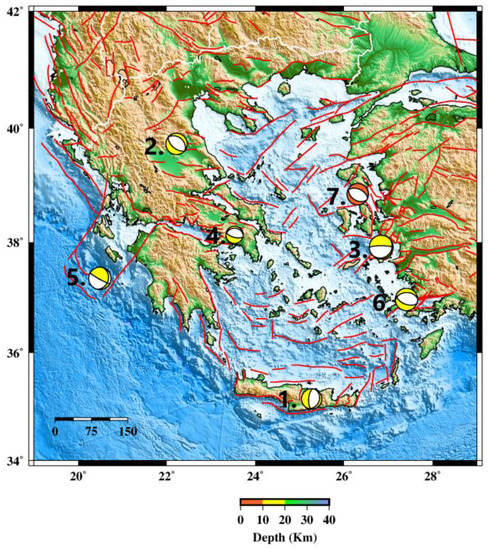
Figure 1.
Geographical distribution of the seven studied mainshocks. The index numbers depicted in this figure correspond to the event indices given in Table 1. The colors and sizes of the focal mechanisms (beachballs) are related to the depth and the magnitude of each event. The faults are visualized according to the GEM database [28].
For the purpose of the definition of the aftershock zone, an elliptical region was initially picked for every main shock based on the distribution of its aftershocks and consequently the catalogue for each aftershock sequence was obtained. In order to test the stability of our results, we examined creating catalogues of earthquakes with 20% greater major axes of the ellipse. Considering the spatial distribution of aftershocks, small changes do not affect the parameter estimations that we will consider below, since the majority of the aftershock events included in the elliptic area first selected. Subsequently, the catalogue was updated to include all earthquake event occurrences inside this zone and for a period of two to four months after the main shock (see Table 1). Following the creation of the catalogues, we estimated the magnitude of completeness (Mc) for each aftershock sequence using the frequency–magnitude distribution [29,30]. It is worth noting that aftershock sequences can be depicted in terms of the modified parameters of the Gutenberg–Richter law [31,32].
The locations of the seven shallow mainshocks are illustrated in Figure 1. The earthquake numbers are presented chronologically from most recent to oldest in the event indexes. Along with the entropic parameters q and Tc, which represent the transition point from the non-additive to additive range in every aftershock series, the parameters of each mainshock and its aftershock sequence are summarized in Table 1.
Next, the interevent time distribution is calculated for each aftershock sequence, and a Q-exponential function fitting up to a value Tc, yielding to the Q and q parameters, respectivelly. In all cases that we study, we observe a deviation from the Q-exponential function for high values of time T, with T > Tc. Additionally, using the estimated Q value from the prior analysis, the Q-logarithmic function of P(>T) as a function of T is constructed. The range of interevent times, provided by Equation (12), where lnQP(>T) vs. T is a straight line, is then specified along with its correlation coefficient. The transition from NESP to BG statistical physics is indicated by the deviation from linearity at Tc. This demonstrates that in the immediate aftermath of the mainshock, the system is controlled by NESP, whereas as the aftershock sequence develops at T > Tc, the system is controlled by BG statistical mechanics.
Figure 2 presents a flowchart of the process behind the non-extensive statistical physics flowchart implemented in the present work.
Figure 2.
This flowchart summarizes the process behind the non-extensive statistical physics model implemented in the present work.
3.1. The Arkalochori Aftershock Sequence
In this section, we investigate the space–time distribution of the main event’s aftershock sequence, which struck the Greek island of Crete at a depth of about 10 km on 27 September 2021 [33,34] The earthquake’s epicenter was located southeast of Heraklion. The mainshock had a magnitude Mw6.0. Based on a detailed examination of the aftershock sequence, as located by the Hellenic Unified Seismological Network (HUSN) station network (http://www.gein.noa.gr/en/networks/husn, accessed on 27 September 2022), the aftershock area encompasses the region between longitudes 25.17° E–25.40° E and latitudes 35.03° N–35.24° N. The aftershocks’ catalogue includes events characterized by magnitudes 2.5 ≤ Mw ≤ 5.8, with a completeness magnitude of Mc = 2.5. According to different networks and catalogues, Mc-value varies systematically in space and time. However, we should be cautious because commonly this value may lead to inaccurate estimations in statistical analyses due to it being higher in the early part of an earthquake sequence.
We study the probability distribution of interevent times in the aftershock series of the Arkalochori, 2021 event using the NESP framework, as described previously. This approach results from the generalized expression of entropy (Equation (1)), which is characteristic for complex systems with finite degrees of freedom and long-range memory [5,8,22].
Figure 3a shows a typical Q-exponential pattern in the log–log plot of the cumulative distribution function (CDF), P(>T) = N(>T)/N0 of aftershocks’ interevent times. Figure 3a shows that for values of T greater than a critical interevent time Tc (i.e., when T > Tc), there is a divergence from the Q-exponential function. Furthermore, fitting the Q-exponential to the instances up to a value near to Tc yields q = 1.62, as shown by Equations (7) and (8).
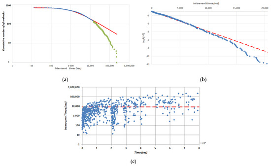
Figure 3.
(a) The interevent times CDF of the 2021 Mw6.0 Arkalochori earthquake, for the aftershocks with M > Mc. The scarlet solid line is the Q-exponential operation with q = 1.62. The change of colors indicates the crossover between the NESP (blue circles) and BG statistics (green triangles). (b) The lnQP(>T) as a function of interevent times T, where the scarlet line presents the fitting with q = 1.62 and correlation coefficient 0.9953 up to Tc. Tc value close to 7750 s is suggested by the deviation from linearity. (c) Interevent time T evolution with time t since the main shock. The red line illustrates the Tc value.
Next, we show lnQP(>T) (see Equation (10)) as a function of interevent times T for q = 1.62 in Figure 3b. We estimate Tc to be ≈7750 s based on the divergence from predicted linearity during the transition from one system to another.
Figure 3c illustrates that the T evolves as a function of time t since the main shock. The Tc value indicates that the majority of interevent times have a value of T below Tc (Figure 3c) in the early aftershock time, supporting the idea that the NESP mechanism is predominant in the beginning of the aftershock evolution, indicating finite degrees of freedom and long-range memory effects. As time passes, these traits of the aftershock sequence are not prevalent anymore and BG statistics are restored (i.e., q = 1) [14].
3.2. The Elassona Aftershock Sequence
Here we focus on the aftershock sequence of the main earthquake that took place near the capital city of Larissa in Thessaly on 3 March 2021. The mainshock had a magnitude of Mw6.0 (from the Geophysical Laboratory of the Aristotle University of Thessaloniki (GL-AUTH), http://geophysics.geo.auth.gr/, accessed on 27 September 2022) (Table 1), and generated a prolonged aftershock sequence in a general SE–NW direction [34]. The aftershock area, for a 1-month time interval from 3 March 2021 to 4 April 2021, covers the region between longitudes 21.47° E–23.13° E and latitudes 39.01° N–40.56° N. The aftershocks’ catalogue includes 676 aftershocks characterized by magnitudes 2.5 ≤ Mw ≤ 5.8, with a completeness magnitude of Mc = 2.5 [33,35].
The CDF of the interevent times for the Elassona 2021 aftershock sequence, based on the fitting of the Q-exponential function (Equations (7) and (8)) to the values of T, up to a value approaching Tc, reaches to q = 1.62 (see Figure 4). Next, in Figure 4b we present the lnQP(>T) as an operation of interevent times T for q = 1.62. From its deviation from the expected linearity, the approximated value of Tc ≈ 4587 s is extracted. A graph of the evolution of interevent time T over time t since the main shock is shown in Figure 4c.
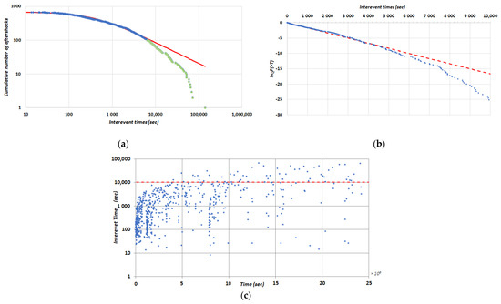
Figure 4.
(a) The interevent times CDF of the 2021 Mw6.3 Elassona Earthquake, for the aftershocks with M > Mc. The scarlet stroke is the Q-exponential fitting with q = 1.62. The change of colors indicates the crossover between the NESP (blue circles) and BG statistics (green triangles). (b) The lnQP(>T) as a function of T, where the scarlet line presents the fitting with q = 1.62 and correlation coefficient 0.9936 up to Tc. Tc value close to 4587 s is suggested by the deviation from linearity. (c) Interevent time T evolution with time t since the main shock. The red line illustrates the Tc value.
3.3. The Samos Aftershock Sequence
A strong and shallow earthquake of Mw = 7.0 struck Samos Island on the Aegean Sea (Figure 1), on 30 October 2020. Its aftershocks area covers the region between longitudes 26.10° E–26.99° E and latitudes 37.64° N–37.98° N. The catalogue, for a completeness magnitude of Mc = 2.5, includes 1158 aftershocks (Table 1).
Using the same methodology as previously, fitting the Q-exponential function to the noticed data up to a value near to Tc yields q = 1.63 (Figure 5a). We estimate Tc to be 9761 s, based on the deviation from predicted linearity (Figure 5b). In the early time aftershock part, most of the interevent times, with T values less than Tc exist, which forces us to conclude that the Tsallis entropy mechanism is dominant in this early part of the aftershock evolution. With the progress of time, the pattern of the aftershock sequence, such as finite degrees of freedom and long-range memory, are notpredominant anymore and the BG statistical physics controls the aftershocks evolution (i.e., q = 1) (Figure 5c) [14].
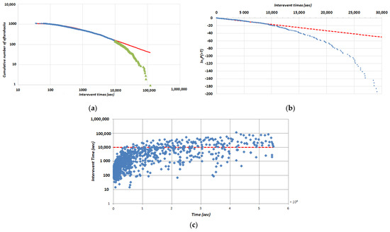
Figure 5.
(a) The interevent times CDF of the 2020 Mw7.0 Samos Earthquake, for the aftershocks with M > Mc. The scarlet solid stroke is the Q-exponential fitting with q = 1.63. The change of colors indicates the crossover between the NESP (blue circles) and BG statistics (green triangles). (b) The lnQP(>T) as a function of T, where the red line presents the fitting with q = 1.63 and correlation coefficient 0.9942 up to Tc. A Tc value close to 9761 s is suggested by the deviation from linearity. (c) Interevent time T evolution with time t since the main shock. The scarlet line illustrates the Tc value.
3.4. The Parnitha Aftershock Sequence
On 19 July 2019, at 11:13:15 GMT (Greenwich Mean Time), an earthquake of Mw = 5.1 struck Athens, the Capital of Greece. The mainshock’s location parameters were obtained from the catalogue of Kapetanidis et al. (2020) [36], summarized in Table 1. The event took place NW of the Thriassio basin. The aftershock distribution of the 436 events covers the region between longitudes 23.47° E–23.67° E and latitudes 38.05° N–38.18° N and characterizes aftershocks with magnitudes 1.0 ≤ Mw ≤ 4.2. The catalogue of this earthquake with completeness magnitude Mc = 1.0, covers the period from the day of the main event up to 21 August 2020.
In Figure 6a, q = 1.71 is obtained by fitting the Q-exponential function to the observed data up to a value close to Tc. In the present aftershock sequence, there is a slight increase in the parameter q compared to the previous ones (see also Table 1). The deviation of the Q-logarithmic operation from the expected linearity is observed at a Tc value of ≈175,460 s (Figure 6b). In the early aftershock period, there are more interevent times with values lower than Tc indicating that the Tsallis entropy description dominates the aftershock evolution in the immediate to the main shock time. As time passes, some of the traits of the early aftershock sequence related to NESP are insignificant and BG statistical physics are recovered.
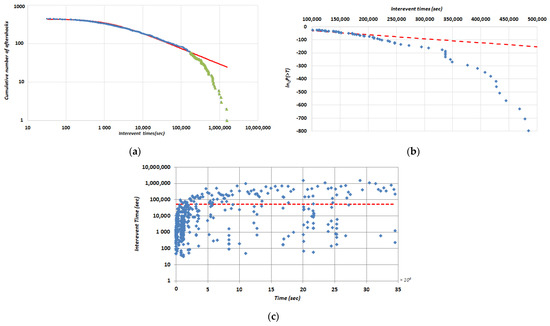
Figure 6.
(a) The interevent times CDF of the 2019 Mw5.1 Parnitha Earthquake, for the aftershocks with M > Mc. The scarlet stroke is the Q-exponential fitting with q = 1.71. The change of colors indicates the crossover between the NESP (blue circles) and BG statistics (green triangles). (b) The lnQP(>T) as a function of T, where the red line is the fitting with q = 1.71 and correlation coefficient 0.9912 up to Tc. Tc value close to 175,460 s is suggested by the deviation from linearity. (c) Interevent time T evolution with time t since the main shock. The scarlet line illustrates the Tc value.
3.5. The Zakynthos Aftershock Sequence
Herein, we study the seismic sequence that began on 25 October 2018 with a shallow Mw = 6.6 earthquake off the coast Zakynthos (Ionian Sea, Greece) (Figure 1). Based on detailed examination of the 1668 aftershock sequence, which were located by the station network of the Hellenic Unified Seismological Network (HUSN), we conclude that the duration corresponds to the 1-year time period i.e., from 25 October 2018 up to 19 October 2019. According to the catalogue used, aftershocks occurred with a magnitude greater than Mw2.1.
Plotting the CDF, P(>T) = N(>T)/N0 of aftershocks interevent times on a double-log scale, a typical Q-exponential pattern presents for T < Tc, with q = 1.68 (Figure 7a). The transition from NESP to BF statistics is estimated to be at about Tc ≈ 5607 s (Figure 7b). The Tc value (red dashed line in Figure 7c) suggests that the Tsallis entropy controls the early stages of the aftershocks’ evolution. Certain traits of the early aftershock sequence related to the NESP become less significant as time passes by, and the statistical physics of BG is recovered.
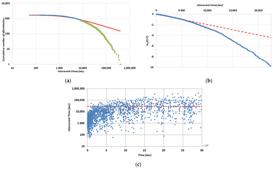
Figure 7.
(a) The interevent times CDF of the 2018 Mw6.6 Zakynthos Earthquake, for the events with M > Mc. The scarlet stroke is the Q-exponential fitting with q = 1.68. The change of colors indicates the crossover between the NESP (blue circles) and BG statistics (green triangles). (b) The lnQP(>T) as a function of T, where the red line is the fitting with q = 1.68 and correlation coefficient 0.9966 up to Tc. Tc value close to 5607 s is suggested by the deviation from linearity. (c) Interevent time T evolution with time t since the main shock. The scarlet line illustrates the Tc value.
3.6. The Kos Aftershock Sequence
An earthquake with magnitude Mw = 6.5 at a depth of 7.1 km, which had a normal faulting mechanism striking about east–west (Figure 1), happened on 20 July 2017 in Gökova Bay, in the Aegean Sea, at 22:31:10 GMT between Bodrum town, Turkey, and Kos Island, Greece. As stated in the data, the mainshock epicenter was given as 27.41° E and 36.97° N located 12 km ENE to Kos in Greece and 8 km SE to Bodrum in Muğla in Turkey. The earthquake generated a tsunami that affected the coast of the Bodrum peninsula and the northeast coast of Kos. A tide gauge in Bodrum, close to the earthquake’s epicenter, recorded the tsunami [37].
The data were obtained from the Boun Koeri Regional Earthquake-Tsunami Monitoring Center, Kandilli Observatory and Earthquake Research Institute (RETMC) (the Turkish Disaster and Emergency Management Presidency, AFAD; Boğaziçi University (KOERI), http://www.koeri.boun.edu.tr/, accessed on 27 September 2022). This study’s goal is to give a thorough region-time analysis with a variety of aftershock attributes such as the parameter q by Tsallis for 6492 aftershocks identified in six months after the mainshock.
In terms of Tsallis Entropy the value of q is equal to q = 1.63 (Figure 8a). Following, the transition estimated to be at Tc ≈ 15,005 s (Figure 8b). The parameter Tc (red dashed line in Figure 7c) shows that the NESP describes the early part of the aftershocks while as time goes on, BG statistics are revealed.
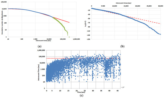
Figure 8.
(a) The interevent times CDF of the 2017 Mw6.5 Kos Earthquake, for the aftershocks with M > Mc. The scarlet line is the Q-exponential fitting with q = 1.63. The change of colors indicates the crossover between the NESP (blue circles) and BG statistics (green triangles). (b) The lnQP(>T) as a function of T, where the red line is the fitting with q = 1.63 and correlation coefficient 0.9935 up to Tc. Tc value close to 15,005 s is suggested by the deviation from linearity. (c) Interevent time T evolution with time t since the main shock. The scarlet line illustrates the Tc value.
3.7. The Mytilene Aftershock Sequence
The 2017 Mytilene earthquake of Mw6.3, took place at the coordinates (26.31, 38.85) (see more for location parameters in the Table 1) on 12 June at 12:28:37 GMT.
This destructive offshore event occurred northeast of Chios and almost 15 km south of the southeast coast of Lesbos. In Vrissa village, a collapsed building killed one person and injured 15 others due to a collapsed building and falling debris. Damage was reported in at least 12 villages across the southeast region of Lesvos, and there was additional impact along the Turkish coast [38]. Regarding the environmental impact of the earthquake, slope displacement and ground cracks occurred in many places in the disaster area. Also, tsunamis were reported in Plomari Port [38].
A total of 1610 aftershocks were detected over the period between 12 June 2017 and 11 June 2018 (European Mediterranean Seismological Centre, EMSC). The aftershock area covers the region between the coordinates by longitudes 25.22° E–27.30° E and latitudes 38.23° N–39.22° N.
In line with the analysis of the previous aftershock sequences, for the earthquake of Mytilene, we study the distribution of the interevent times. The value of q is equal to q = 1.68 (Figure 9a). The transition estimated to be at Tc ≈ 10,761 s (Figure 9b). Since the most interevent times have T values T < Tc, the parameter Tc (red dashed line in Figure 9c) confirms that the Tsallis entropy description dominates the early stages of the aftershocks’ evolution.
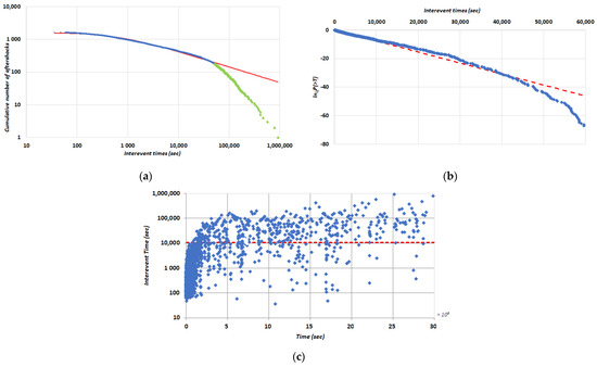
Figure 9.
(a) The interevent times CDF of the 2017 Mw6.3 Mytilene Earthquake, for the aftershocks with M > Mc. The scarlet line is the Q-exponential fitting with q = 1.68. The change of colors indicates the crossover between the NESP (blue circles) and physical BG statistics (green triangles). (b) The lnQP(>T) as a function of T, where the red line is the fitting with q = 1.68 and correlation coefficient 0.9927 up to Tc. Tc value close to 10,761 s is suggested by the deviation from linearity. (c) Interevent time T evolution with time t since the main shock. The scarlet line illustrates the Tc value.
In addition, and for all the aftershock sequences that were studied, we introduce a normalized parameter, x = T/Tc, where x < 1 indicates the range where the Tsallis entropy describes the evolution of aftershocks sequence interevent times, while x > 1 is related to the Boltzmann–Gibbs (BG) process. This is because P(>T) = expQ(−T/T*) for T < Tc. A deviation from the Q-exponential is present for all of the examined aftershock sequences when x >> 1 (i.e., T >> Tc). An inspection of Figure 10, where all aftershock sequences are plotted together, suggests that for 0.01 < x < 1, power-law scaling emerges for all the aftershock sequences, with a slope in the range 0.40–0.60, conforming to the q values calculated from the analysis (Table 1). The latter is expected since the asymptotic expression of Equation (6) is is a typical expression of a power law.
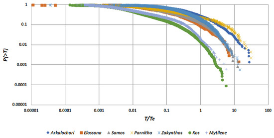
Figure 10.
The interevent times distribution P(>x) for all the studied aftershock sequences as a function of x = T/Tc. Deviations from the Q-exponential operation are pronounced at T/Tc >> 1, for all sequences.
It is important to mention, that in all estimations the accuracy of the estimated values is in the order of ±0.01.
4. Discussion
All shallow earthquakes are followed by an aftershock sequence. The statistical properties of aftershock sequences are associated with scaling relations such as that extracted in view of non-extensive statistical physics (NESP). In this study, we used a detailed temporal assessment of the aftershock sequences over the last five years of significant earthquakes in Greece with magnitudes that reach up to Mw = 7.0. We studied the strong events, such as the Mw6.0 Arkalochori (27 September 2021), the Mw6.3 Elassona (3 March 2021), the Mw7.0 Samos (30 October 2020), the Mw5.1 Parnitha (19 July 2019), the Mw6.6 Zakynthos (25 October 2018), the Mw6.5 Kos (20 July 2017) and the Mw6.1 Mytilene (12 June 2017) earthquakes. Based on non-expansive statistical physics, we analyzed the distribution of interevent times for each aftershock sequence for each main shock.
In all cases, the cumulative distribution function P(>T) is defined by a Q-exponential in the early stage of the aftershock sequence where interevent times less than Tc are observed, where Tc is the crossover point between the non-additive and additive behavior. By fitting a Q-exponential function to the data up to a value close to Tc, the parameter q is estimated for each aftershock sequence. In all the cases analyzed, the applicability of non-extensive statistical physics to the interevent times CDF is demonstrated, as well as, the existence of transition behavior from the power-law to exponential scaling for larger interevent times. Since the q entropic parameter is greater than one (q > 1) a sub-additive process is implied, supporting the conclusion that long-range memory exists in the early state of temporal evolution of aftershocks where mainly T < Tc. Additionally, for aftershock sequences analyzed, the estimated Tsallis entropic q-values that describe the observed CDF are within the range of 1.62–1.71.
In addition, the superposition of two aftershock mechanisms can be used to explain the observed scaling behavior and the deviation from the Q-exponential function for greater interevent times. For T > Tc, a second mechanism—characterized by an exponential function—becomes apparent. The first mechanism, as presented by NESP, is dominant for T < Tc. We, thus, introduce the generalization described in [20,39,40], to account for a transition from NESP (q ≠ 1) to BG (q = 1) statistical mechanics, where:
whose solution is
In Equation (13) the probability function p(T) decreases monotonically with increasing T for positive βq and β1, where C is a normalization factor. As a result, when (q−1)β1 << 1, a q-exponential, , where , is an approximation of Equation (13), while for (q − 1)β1 >> 1, the asymptotic behavior of the probability distribution function , is an exponential one, where Tc = 1/(q − 1)β1 defines the crossover point from the non-additive to additive behavior [24,41]. The Tc value suggests that the Tsallis entropy is prevalent in the early stages of aftershock evolution, while the traits of aftershock sequences which are associated with a NESP description, become less apparent as time passes and BG statistics are recovered [6,9,17,22,42,43].
The super-statistical theory, which is complementary to NESP, is based on a superposition of ordinary local equilibrium statistical mechanics, with a Gamma distributed intensive parameter that varies over a fairly wide time scale. This approach can be used to explain the q-exponential behavior of the interevent times in aftershock sequences [14].
The super-statistical approach states that the interevent times of an aftershock sequence may be described by a local Poisson process , with β an intensive fluctuating parameter. On a long-time scale, β is distributed with a possibility density f(β) [25,44,45,46,47]. Then the probability distribution p(T) is given as:
In the scenario where a Gamma distribution provides the probability density of β [43,44,45,46]:
Integration of Equation (14) is analytically calculated [48], obtained , which is exactly the result in term of NESP, where q = 1 + ([2⁄(n + 2)]) and [14]. Since in all the analyzed cases q is in the range 1.61–1.71, we conclude that the corresponding number of degrees of freedom is close to one (n = 1).
The latter implies that the evolution of an aftershock sequence could be influenced by a stochastic mechanism with memory effects. In accordance with [49,50], the stochastic differential equation for the evolution with time t, of interevent times T of an aftershock sequence:
This stochastic equation is made up of two parts that control how the seismicity evolves. The primary goal of the first deterministic term is to restore the seismic rate R to its usual value of R = 1/<T> based on a constant γ which expresses the rate of relaxation to the mean waiting time <T>. Memory effects in seismicity’s development are depicted in the second stochastic part. The stochastic term Wt describes a Wiener process following a Gaussian distribution with zero mean and unitary variance that could follow the macroscopic effects in the evolution of interevent times in the aftershock sequence. Wt’ random sign causes an increase (Wt > 0) or decrease (Wt < 0) of T. The construction of this term operates in a way that large values of T cause large amplitude of the stochastic term, which leads to an increase or decrease in T depending on the sign of Wt. The parameter φ introduces a noise component to the process and can be expressed as [50].
Equation (16) is a stochastic differential equation that represents a multiplicative noise example, known as the Feller process [48,49,50].
We write the corresponding Fokker–Planck equation for Equation (16), to ascertain the evolution of the interevent time series T after some time t, given the probability distribution f(T, t), as [51]:
The latter Fokker–Planck equation’s stationary solution, Equation (17), is the distribution [48]:
where Equation (18) presents the conditional probability of T given <T>.
It is necessary to account for local variations in the seismic rate R = 1/<T> associated with non-stationarities in the evolution of the earthquake activity over time scales significantly larger than 1/γ in order to achieve stationarity in Equation (16). In this case, the mean interevent time <T> exhibits local variations, and we assume that these fluctuations adhere to the stationary gamma distribution:
where Equation (19) gives the marginal probability of T, [52] as:
The latter integration leads to:
By continuing to implement the variable changes:
and taking into account the form of q-exponential function in Equation (2), Equation (16) can be transformed to [50]:
which is the exact form of the q-exponential function.
5. Concluding Remarks
In summarizing the study’s findings, we concentrated on analyzing the distributions of interevent times for each sequence in order to statistically examine its patterns in the most recent aftershock sequences in Greece.
Namely:
- We can state that the aftershock sequences located in Greece follows the statistical mechanics model derived in the framework of Non-Extensive Statistical Physics (NESP);
- Moreover, we should note that the NESP approach is useful for other regions, not only for the Greek territory, such as subduction zones all over the word [53];
- According to the NESP approach used here, it suggests that the system is in an abnormal equilibrium with a transition for large interevent times from abnormal (q > 1) to normal (q = 1) statistical mechanics;
- The analysis of the interevent times distribution indicates such a system;
- The range of the non-extensive parameter q and for all sequences studied, results in a non-extensive entropic parameter q with a range of between 1.62 and 1.71, which suggests a system with one degree of freedom.
To summarize, the used models fit the noticed distributions reasonably well, and imply the importance of using NESP in evaluating such phenomena.
The main limitations of the work presented in this paper are related to earthquakes in different geotectonic environments along with fault types of the main shock. Studying aftershock sequences as a function of geotectonic environments is a matter of discussion in future studies, and this could be useful for the prediction of damaged aftershocks [54,55,56,57].
Author Contributions
Conceptualization, F.V.; methodology, F.V., E.-A.A., S.-E.A., G.M.; software, G.M. and E.-A.A.; validation, E.-A.A. and S.-E.A.; formal analysis, F.V., E.-A.A., S.-E.A., G.M.; investigation, F.V., E.-A.A., S.-E.A., G.M.; resources, F.V., E.-A.A., S.-E.A., G.M.; data curation, F.V., E.-A.A., S.-E.A., G.M.; writing—original draft preparation, F.V., E.-A.A., S.-E.A., G.M.; writing—review and editing, F.V., E.-A.A., G.M.; visualization, F.V., E.-A.A.; supervision, F.V. All authors have read and agreed to the published version of the manuscript.
Funding
This research received no external funding.
Data Availability Statement
Data are available at the Hellenic Unified Seismic Network (H.U.S.N., http://www.gein.noa.gr/en/networks/husn), (A.U.TH.: Aristotle University of Thessaloniki [http://geophysics.geo.auth.gr/ss/], E.M.S.C.: European Mediterranean Seismological Centre [https://www.emsc-csem.org/#2], N.K.U.A.: National and Kapodistrian University of Athens [http://www.geophysics.geol.uoa.gr/], K.O.E.R.I.: Kandilli Observatory and Earthquake Research Institute [http://www.koeri.boun.edu.tr/new/en]. Last visit to the above webpages: 12 September 2022.
Acknowledgments
We would like to thank Andreas Karakonstantis for his valuable assistance in the construction of the seismotectonic map.
Conflicts of Interest
The authors declare no conflict of interest.
References
- Telesca, L.; Cuomo, V.; Lapenna, V.; Vallianatos, F.; Drakatos, G. Analysis of the temporal properties of Greek aftershock sequences. Tectonophysics 2001, 341, 163–178. [Google Scholar] [CrossRef]
- Papazachos, B.C.; Papazachou, C. The Earthquakes of Greece; Ziti Publications: Thessaloniki, Greece, 2003. [Google Scholar]
- Tsapanos, T. Seismicity and Seismic Hazard Assessment in Greece; Springer Science: Thessaloniki, Greece, 2008. [Google Scholar]
- Kassaras, I.; Kapetanidis, V.; Ganas, A.; Tzanis, A.; Kosma, C.; Karakonstantis, A.; Valkaniotis, S.; Chailas, S.; Kouskouna, V.; Papadimitriou, P. The New Seismotectonic Atlas of Greece (v1.0) and Its Implementation. Geosciences 2020, 10, 447. [Google Scholar] [CrossRef]
- Vallianatos, F.; Michas, G.; Papadakis, G. Non-Extensive Statistical Seismology: An Overview. Complex. Seism. Time Ser. 2018, 25–60. [Google Scholar] [CrossRef]
- Michas, G.; Vallianatos, F. Scaling properties, multifractality and range of correlations in earthquake timeseries: Are earth-quakes random? In Statistical Methods and Modeling of Seismogenesis; Limnios, N., Papadimitriou, E., Tsaklidis, G., Eds.; ISTE John Wiley: London, UK, 2021. [Google Scholar] [CrossRef]
- Vallianatos, F.; Sammonds, P. Evidence of non-extensive statistical physics of the lithospheric instability approaching the 2004 Sumatran-Andaman and 2011 Honshu mega-earthquakes. Tectonophysics 2013, 590, 52–58. [Google Scholar] [CrossRef]
- Tsallis, C. Introduction to Non-Extensive Statistical Mechanics: Approaching a Complex World; Springer: Berlin/Heidelberg, Germany, 2009; pp. 41–218. [Google Scholar] [CrossRef]
- Sobyanin, D.N. Generalization of the Beck-Cohen superstatistics. Phys. Rev. E 2011, 84, 051128. [Google Scholar] [CrossRef]
- Vallianatos, F.; Karakostas, V.; Papadimitriou, E. A Non-Extensive Statistical Physics View in the Spatiotemporal Properties of the 2003 (Mw6.2) Lefkada, Ionian Island Greece, Aftershock Sequence. Pure Appl. Geophys. 2013, 171, 1443–1449. [Google Scholar] [CrossRef]
- Efstathiou, A.; Tzanis, A.; Vallianatos, F. On the nature and dynamics of the seismogenetic systems of North California, USA: An analysis based on Non-Extensive Statistical Physics. Phys. Earth Planet. Inter. 2017, 270, 46–72. [Google Scholar] [CrossRef]
- Vallianatos, F.; Michas, G.; Papadakis, G.; Tzanis, A. Evidence of non-extensivity in the seismicity observed during the 2011–2012 unrest at the Santorini volcanic complex, Greece. Nat. Hazards Earth Syst. Sci. 2013, 13, 177–185. [Google Scholar] [CrossRef]
- Vallianatos, F.; Michas, G.; Papadakis, G.; Sammonds, P. A Non-Extensive Statistical Physics View to the Spatiotemporal Properties of the June 1995, Aigion Earthquake (M6.2) Aftershock Sequence (West Corinth Rift, Greece). Acta Geophys. 2012, 60, 759–765. [Google Scholar] [CrossRef]
- Vallianatos, F.; Pavlou, K. Scaling properties of the Mw7.0 Samos (Greece), 2020 aftershock sequence. Acta Geophysica 2021, 69, 1067–1084. [Google Scholar] [CrossRef]
- Sychev, V.N.; Sycheva, N.A. Nonextensive analysis of aftershocks following moderate earthquakes in Tien Shan and North Pamir. J. Volcanol. Seismol. 2021, 15, 58–71. [Google Scholar] [CrossRef]
- Michas, G.; Papadakis, G.; Vallianatos, F. A Non-Extensive approach in investigating Greek seismicity. Bull. Geol. Soc. Greece 2013, 47, 1177–1187. [Google Scholar] [CrossRef]
- Vallianatos, F.; Telesca, L. Application of Statistical Physics in Earth Sciences and Natural Hazards. Acta Geophys. (Spec. Issue) 2012, 60, 499. [Google Scholar] [CrossRef]
- Tsallis, C. Possible generalization of Boltzmann-Gibbs statistics. J. Stat. Phys. 1988, 52, 479–487. [Google Scholar] [CrossRef]
- Telesca, L. Maximum likelihood estimation of the non-extensive parameters of the earthquake cumulative magnitude distribution. Bull. Seismol. Soc. Am. 2012, 102, 886–891. [Google Scholar] [CrossRef]
- Vallianatos, F.; Michas, G.; Papadakis, G. Non-Extensive Statistical Seismology: An overview. In Complexity of Seismic Time Series: Measurement and Application, 1st ed.; Chelidze, T., Vallianatos, F., Telesca, L., Eds.; Elsevier: Amsterdam, The Netherlands, 2018; pp. 25–53. [Google Scholar]
- Vallianatos, F.; Papadakis, G.; Michas, G. Generalized statistical mechanics approaches to earthquake and tectonics. Proc. R. Soc. A 2016, 472, 20160497. [Google Scholar] [CrossRef]
- Abe, S.; Suzuki, N. Scale-free statistics of time interval between successive earthquakes. Physica A 2005, 350, 588–596. [Google Scholar] [CrossRef]
- Abe, S.; Suzuki, N. Scale-invariant statistics of period in directed earthquake network. Eur. Phys. J. B 2005, 44, 115–117. [Google Scholar] [CrossRef]
- Tsallis, C. Nonadditive entropy and non-extensive statistical mechanics—An overview after 20 years. Brazil. J. Phys. 2009, 39, 337–339. [Google Scholar] [CrossRef]
- Beck, C. Superstatistical Brownian Motion. Prog. Theor. Phys. Suppl. 2006, 162, 29–31. [Google Scholar] [CrossRef]
- Vallianatos, F.; Benson, P.; Meredith, P.; Sammonds, P. Experimental evidence of a non-extensive statistical physics behavior of fracture in triaxially deformed Etna basalt using acoustic emissions. EPL 2012, 97, 58002. [Google Scholar] [CrossRef]
- Telesca, L. Tsallis-Based Nonextensive Analysis of the Southern California Seismicity. Entropy 2011, 13, 1267–1280. [Google Scholar] [CrossRef]
- Caputo, R.; Pavlides, S. The Greek Database of Seismogenic Sources (GreDaSS), Version 2.0.0: A Compilation of Potential Seismogenic Sources (Mw > 5.5) in the Aegean Region. 2013. Available online: https://gredass.unife.it/ (accessed on 26 October 2022).
- Gutenberg, B.; Richter, C.F. Magnitude and energy of earthquakes. Ann. Geophys. 1956, 9, 1–15. [Google Scholar] [CrossRef]
- Wyss, M.; Wiemer, S.; Zuniga, R. Zmap: A Tool for Analyses of Seismicity Patterns, Typical Applications and Uses: A Cookbook. Available online: http//:www.researchgate.net/publication/261508570_cookbook (accessed on 26 October 2022).
- Avgerinou, S.-E.; Anyfadi, E.-A.; Michas, G.; Vallianatos, F. Study of the Frequency Magnitude Distribution of recent Aftershock Sequences of Earthquakes in Greece, in Terms of Tsallis Entropy. In Proceedings of the 16th International Congress of the Geological Society of Greece, Patras, Greece, 17–19 October 2022. [Google Scholar]
- Avgerinou, S.-E. A Non-Extensive Statistical Physics View to the Temporal Properties of the Recent Aftershock Sequences of Strong Earthquakes in Greece. Master’s Thesis, Earth Science Department of Geology and Geoenviroment, Athens, Greece, 2021. [Google Scholar]
- Vallianatos, F.; Michas, G.; Hloupis, G. Seismicity Patterns Prior to the Thessaly (Mw6. 3) Strong Earthquake on 3 March 2021 in Terms of Multiresolution Wavelets and Natural Time Analysis. Geosciences 2021, 11, 379. [Google Scholar] [CrossRef]
- Vallianatos, F.; Karakonstantis, A.; Michas, G.; Pavlou, K.; Kouli, M.; Sakkas, V. On the Patterns and Scaling Properties of the 2021–2022 Arkalochori Earthquake Sequence (Central Crete, Greece) Based on Seismological, Geophysical and Satellite Observations. Appl. Sci. 2022, 12, 7716. [Google Scholar] [CrossRef]
- Michas, G.; Pavlou, K.; Avgerinou, S.-E.; Anyfadi, E.-A.; Vallianatos, F. Aftershock patterns of the 2021 Mw 6.3 Northern Thessaly (Greece) earthquake. J. Seismol. 2022, 26, 201–225. [Google Scholar] [CrossRef]
- Kapetanidis, V.; Karakonstantis, A.; Papadimitriou, P.; Pavlou, K.; Spingos, I.; Kaviris, G.; Voulgaris, N. The 19 July 2019 earthquake in Athens, Greece: A delayed major aftershock of the 1999 Mw = 6.0 event, or the activation of a different structure? J. Geodyn. 2020, 139, 101766. [Google Scholar] [CrossRef]
- Öztürk, S.; Şahin, S. A statistical space-time-magnitude analysis on the aftershocks occurrence of the 21 July 2017 MW = 6.5 Bodrum-Kos, Turkey, earthquake. J. Asian Earth Sci. 2018, 172, 443–457. [Google Scholar] [CrossRef]
- Lekkas, E.; Voulgaris, N.; Karydis, P.; Tselentis, G.-A.; Skourtsos, E.; Antoniou, V.; Andreadakis, E.; Mavroudis, S.; Spirou, N.; Speis, F.; et al. Prelιminary Report, Lesvos Earthquake Mw 6.3, 12 June 2017, Environmental, Disaster and Crisis Management Strategies. Available online: https://paleoseismicity.org/ (accessed on 30 September 2022).
- Vallianatos, F. A non-extensive statistical physics approach to the polarity reversals of the geomagnetic field. Phys. A Stat. Mech. Appl. 2011, 390, 1773–1778. [Google Scholar] [CrossRef]
- Sugiyama, M. Introduction to the topical issue: Nonadditive entropy and non-extensive statistical mechanics. Continuum Mech. Thermodyn. 2004, 16, 221–222. [Google Scholar] [CrossRef]
- Vallianatos, F.; Sammonds, P. Is plate tectonics a case of non-extensive thermodynamics? Phys. A Stat. Mech. Appl. 2010, 389, 4989–4993. [Google Scholar] [CrossRef]
- Chochlaki, K.; Vallianatos, F.; Michas, G. Global regionalized seismicity in view of Non-Extensive Statistical Physics. Phys. A Stat. Mech. Appl. 2018, 493, 276–285. [Google Scholar] [CrossRef]
- Beck, C. Superstatistics: Theory and applications. Continum Mech. Thermodyn 2004, 16, 294–298. [Google Scholar] [CrossRef]
- Beck, C. Recent developments in superstatistics. Braz. J. Phys. 2009, 39, 357–362. [Google Scholar] [CrossRef]
- Beck, C. Dynamical Foundations of Nonextensive Statistical Mechanics. Phys. Rev. Lett. 2001, 87, 180601. [Google Scholar] [CrossRef]
- Beck, C.; Cohen, E.G.D. Superstatistics. Physica A 2003, 322, 267–269. [Google Scholar] [CrossRef]
- Antonopoulos, C.G.; Michas, G.; Vallianatos, F.; Bountis, T.; Physica, A. Evidence of q-exponential statistics in Greek seismici-ty. Phys. A Stat. Mech. Appl. 2014, 409, 71–77. [Google Scholar] [CrossRef]
- Mathai, A.M. A pathway to matrix-variate gamma and normal densities. Lin. Al. Appl. 2005, 396, 317–328. [Google Scholar] [CrossRef]
- Feller, W. Two Singular Diffusion Problems. An. Math 1951, 54, 173–182. [Google Scholar] [CrossRef]
- Michas, G.; Vallianatos, F. Stochastic modeling of nonstationary earthquake time series with long-term clustering effects. Phys. Rev. E 2018, 98, 042107. [Google Scholar] [CrossRef]
- Gardiner, C.W. Handbook of Stochastic Methods for Physics, Chemistry, and the Natural Sciences, 1st ed.; Springer: Berlin/Heidelberg, Germany, 1993. [Google Scholar]
- Risken, H. The Fokker-Planck Equation: Methods of Solution and Applications, 2nd ed.; Springer: Berlin, Heidelberg, 1989. [Google Scholar] [CrossRef]
- Anyfadi, E.-A.; Avgerinou, S.-E.; Michas, G.; Vallianatos, F. Universal Non-Extensive Statistical Physics Temporal Pattern of Major Subduction Zone Aftershock Sequences. Entropy 2022, 24, 1850. [Google Scholar] [CrossRef] [PubMed]
- Yeo, G.L.; Allin Cornell, C. A probabilistic framework for quantification of aftershock ground-motion hazard in California: Methodology and parametric study. Wiley Online Libr. Earthq. Eng. Struct. Dyn. 2008, 38, 45–60. [Google Scholar] [CrossRef]
- Jayaram, N.; Baker, J.-W. Correlation model for spatially distributed ground-motion intensities. Wiley Online Libr. Earthq. Eng. Struct. Dyn. 2009, 38, 1687–1708. [Google Scholar] [CrossRef]
- Asim, K.-M.; Martínez-Álvarez, F.; Basit, A.; Iqbal, T. Earthquake magnitude prediction in Hindukush region using machine learning techniques. SpringerLink Nat. Hazards 2017, 85, 471–486. [Google Scholar] [CrossRef]
- Melgarejo-Morales, A.; Vazquez-Becerra, G.E.; Millan-Almaraz, J.-R.; Pérez-Enríquez, R.; Martínez-Félix, C.-A.; Ramon Gaxiola-Camacho, J. Examination of seismo-ionospheric anomalies before earthquakes of Mw ≥ 5.1 for the period 2008–2015 in Oaxaca, Mexico using GPS-TEC. SpringerLink Solid Earth Sci. Acta Geophys. 2020, 68, 1229–1244. [Google Scholar] [CrossRef]


Disclaimer/Publisher’s Note: The statements, opinions and data contained in all publications are solely those of the individual author(s) and contributor(s) and not of MDPI and/or the editor(s). MDPI and/or the editor(s) disclaim responsibility for any injury to people or property resulting from any ideas, methods, instructions or products referred to in the content. |
© 2023 by the authors. Licensee MDPI, Basel, Switzerland. This article is an open access article distributed under the terms and conditions of the Creative Commons Attribution (CC BY) license (https://creativecommons.org/licenses/by/4.0/).