Abstract
Atherosclerosis and aneurysm are two non-communicable diseases that affect the human arterial network. The arterioles undergo dimensional changes that prominently influence the flow of oxygen and nutrients to distal organs and organ systems. Several studies have emerged discussing the various possibilities for the circumstances surrounding the existence of these pathologies. In the present work, we analyze the flow of blood across the stenosis and the aneurysmic sac in contrast with the flow of water to explore alterations in the flow characteristics caused by introduction of the graphene layer. We investigate the blood flow past the graphene layer with varying porosity. The study is undertaken to replace usage of a stent along a blocked artery by inserting a thin layer of graphene along the flow channel in the post-pathological section of the geometry. To explain the flow, a 2D mathematical model is constructed, and the validity and exclusivity of the model’s solution are examined. When the artery wall is assumed to be inelastic, the computation of the mathematical system is evaluated using a finite element method (FEM) solver. We define a new parameter called critical porosity to explore the flow possibilities through the graphene layer. The findings indicate that the flow pattern was adversely affected by the graphene layer that was added to the flow field. The negative impact on the flow could be due to the position of the graphene layer placed. The values for the flow of blood across healthy arteriole, stenosed arteriole, and aneurysmic arteriole segments were and respectively. The critical porosity values were achieved with precision in terms of linear errors , , and , respectively. The consequences of the present study disclose various possible ways to utilize graphene and its compounds in the medical and clinical arena, with a prior exploration of the chemical properties of the compound. The idea and the methodology applied for the present study are novel as there have been no previous research works available in this direction of the research field.
1. Introduction
Even while coronary bypass surgery and stenting only work to clear blocked arteries, additional atherosclerotic plaques can still cause issues. Reducing atherosclerotic potential risks is more crucial than ever after surgery to open a blockage. Acting as a conduit for blood flow, a stent comprised of a delicate, malleable mesh tube is inserted into a blood vessel where an aneurysm has developed. The blood flow is abruptly switched away from the aneurysm by this procedure. By reconfiguring the blood flow, the aneurysm is relieved of pressure, which reduces the risk of a rupture. However, application of bare-metal stents increases the chance of arterial re-narrowing. Furthermore, stents are susceptible to clot formation even after the surgery. A myocardial attack may result from these clots closing the artery. In the present research, we intend to analyze and explore an alternate way to deal with stenosis lumps and aneurysmatic bulges by inserting a narrow layer of graphene along the flow channel.
A collection of several clinical and computational studies on the flow of blood across a stented geometry is presented below in order to infiltrate the topic of the present study. Dowlati et al. [1] provided case reports of two patients who had pipeline flow diversion for unruptured cerebral aneurysms. The goal of the trial was to reduce the risks of thromboembolic consequences by focusing on perioperative dual antiplatelet treatment. After receiving cilostazol medication, luminal narrowing significantly improved, and in-stent stenosis resolved, according to a postoperative digital subtraction angiography (DSA). Blood flow via stented vessels was examined by Shafiullah et al. [2]. In this work, the femoral artery underwent Computational Fluid Dynamics (CFD) analysis with blood flow taken into account as a pulsing, incompressible, and Newtonian flow across a realistic velocity waveform. It was shown that the obstruction may enlarge due to unfavorable flow fields that form upstream and downstream of the blockage. The likelihood of restenosis was significantly influenced by the stent’s design as well. Such several studies have been conducted by researchers in the past few decades. Stents deployed are known to damage the sheath of the vessel into which the insertion is made. Hence a novel biomedical way to either deviate from the flow or change the flow characteristics needs to be discovered to avoid the damages caused by stent deployment. The idea of replacing a stent with a layer of chemical compound with biochemical properties is considered in the present manuscript. This is a novel idea for the medical field and a developing milestone is placed here to explore the field in this direction.
One of the abundant elements that is a key ingredient for the existence of life on earth is carbon. Due to its unique electronic structure, carbon undergoes a formation of its allotrope in the form of a single layer of atoms arranged in a two-dimensional honeycomb lattice nanostructure called graphene. For numerous decades, theoretical research on the thermodynamic stability of two-dimensional crystals has suggested that isolation of graphene monolayers was unattainable [3]. A significant advance in this area was taken in 2004 by a Manchester research team led by Geim and Novoselov, who described a method for creating single-layer graphene on a silicon oxide substrate by peeling the graphite using micromechanical cleavage [4]. Graphene revealed exceptional structural, electrical, and mechanical capabilities, and Novoselov and Geim were awarded the Nobel Prize in Physics six years later “for revolutionary discoveries with the two-dimensional substance graphene”. Several ways of producing graphene monolayers have been developed throughout this period [5,6,7]. Because of its 2D allotropic nature, it may be applied in a variety of biological domains. Graphene and its composites have medicinal uses such as gene and micromolecule medication delivery. Graphene is also utilized for protein biofunctionalization, anticancer treatment, and as an antibacterial agent for bone and tooth implantation. The newly synthesized nanomaterials’ biocompatibility enables extensive usage in medicine and biology [1,2,8,9].
The structural, electrical, thermodynamic, visual, physiological, and biochemical characteristics of graphene-based nanocomposites are exceptional. The effects of graphene loading on the mechanical, thermal, and biological properties of graphene nanocomposites were investigated by Rade et al. [10]. The researchers predicted that the addition of graphene would enhance the mechanical and thermal properties of the poly vinyl alcohol/graphene (PVA/Gr) nanocomposite compared to pure poly vinyl alcohol, as well as provide significant antimicrobial activity against the bacterial strain Staphylococcus aureus. By 3-[4,5-dimethylthiazol-2-yl]-2,5 diphenyl tetrazolium bromide (MTT) experiment, the PVA/Gr nanocomposite proved non-cytotoxic to healthy peripheral blood mononuclear cells, demonstrating its great potential for biocompatibility. The inherent nature of graphene flakes on water molecules was explored by Priyanka et al. [11]. To completely understand graphene behavior in water, the researchers examined graphene distortion in the presence of water molecules. The researchers discovered that graphene folded to wrap around water molecules and avoided full failure, as witnessed in the example of a single graphene layer. The findings of this work have been considered an important milestone toward the problem formulation and analysis of the current research work. The biological interactions of graphene and graphene-composed nanomaterials were reviewed by Sanchez et al. [12]. The study determined that full nanomaterial characterization and mechanical toxicity investigations are required for safe and secure graphene nanosheet development and production in order to optimize biomedical applications with the lowest hazards to environmental health and safety. Rivera-Briso et al. [13] analyzed the increased efficiency of poly(3-hydroxybutyrate-co-3-hydroxy valerate) films due to the addition of graphene oxide (GO) nanosheets. The team concluded that the antimicrobial and proliferative activities of the films are enhanced by the inclusion of GO nanosheets. A review of the electrical and gas-sensing properties of reduced graphene is made by Thejas et al. [14].
A comprehensive evaluation of the aforementioned research papers, as well as a few more supporting pieces of documentation published in the literature, uncovers that none of the researchers have attempted the present problem previously, despite the fact that the ideas and research methods described in this paper can be expected to lead to tremendously legendary interconnection across disciplines. The extracted literature mainly deals only with the flow of graphene nanofluids along the flow geometry whereas, in the current manuscript, an attempt to visualize the flow of water and blood across a graphene layer of varying porosity is made concerning the arterial flow geometries with atherosclerotic and aneurysmic abnormalities. Validation of the present manuscript is implemented using the previously published articles on fluid flow, preferably blood flow, across a pathologized arterial segment. As the study is in its preparatory stage, investigation of the flow across the graphene layer is conducted for a simple geometry without considering its elastic nature. More flow problems in various geometries can be seen in [15,16,17,18,19,20,21,22,23,24,25,26,27,28,29,30,31,32,33,34,35].
The present study is at its meristematic stage. The study of flow along arterioles is being considered for the first time and the flow of blood across a layer of a chemical compound is considered a novel idea. Hence, we intend to present the results of the study at its budding stage in the present manuscript. The geometry considered for the present study is analogous to an arteriole segment. Arterioles are the smallest blood vessels that branch out from the arteries. Since a segment of arteriole is considered, we approximate it to a linear geometrical segment with an inelastic wall. The future implications of the present study are clearly stated in the conclusion section of the manuscript.
The present manuscript has been segregated into several sections. Section 2 deals with formation of the mathematical model governing the fluid flow across the graphene layer. It serves as an integrated section of the mathematical model, mathematical analysis of the model by weak formulation, details of the geometry, mesh construction, and mesh independence analysis. Section 3 exhibits the results obtained in solving the partial differential equation (PDE) system using the Finite Element Method (FEM) solver. The results comprise 2D simulation surface images, and 1D-velocity, pressure, and wall shear stress (WSS) curves. Finally, a conclusion is presented with the mention of future study scope as well as the clinical significance of the present work.
2. Mathematical Model and Analysis
Traditionally, numerical approaches have been used to solve models that describe biological systems since they are typically too complicated to be solved analytically. Once a mathematical model is developed, the biological system may simply mimic the reaction to various conditions attributable to the computational technology currently accessible for solving mathematical equations. However, it might not be possible to include all the microscopic features in the mathematical model created, given the broad biology theories already in existence. Determining the assumptions used to frame the mathematical model becomes necessary. In the present manuscript, a few assumptions concerning the problem are regarded to make it meaningful and also informative [36,37].
Although the activity of the heart is periodic, we consider the stationary study of the flow problem as the blood is considered to be Newtonian for the present investigation [38].
- It is presumed that the walls of the arteries are elastic [39].
- The only driving force behind the flow is assumed to be the pressure gradient force.
- It is also assumed that the occurrence of either stenosis or aneurysm is only in the post-graphene region.
The flow across the aneurysmal ballooning along the abdominal aortal wall is governed by the standard Navier–Stokes momentum equation conjugated with the continuity equation. The governing equations are given in Appendix A [40].
Now, the model formulated is investigated mathematically for existence of a solution as well as its uniqueness. We convert the model to a weak form by using the standard results and principles of functional analysis. Weak formulations provide useful tools for analyzing mathematical equations because they allow the application of linear algebra principles to problems in other domains, such as partial differential equations. The principles of functional analysis utilized for the present study are tabulated in Appendix B.
2.1. Existence of a Weak Solution
Weak formulation of the governing equations mentioned above can be obtained by multiplying the Navier–Stokes momentum equation with the test function taken from the test space with vanishing divergence, integrating over the domain of interest. Applying the Gauss formula as a subsequent step, we obtain
Definition 1.
Let be a subspace of . Let . Then the function with belonging to the dual space is said to be a weak solution or a variational solution of Navier–Stokes equation corresponding to the initial value of considered, if +, for all test functions, picked from the space and almost all values of time from the open interval , .
To achieve a sufficiently smooth solution to the momentum equations, we replace by to obtain,
where the pressure term can be reconstructed by the principles considered by Abels et al. [41].
The second and third terms of the left-hand side vanish. Integrating the resultant expression concerning time variable t, we get
This depicts the Energy equality for the problem under consideration. For a three-dimensional system, the above equality gains a weak form (energy inequality).
Theorem 1.
Let be a bounded domain and satisfies the assumptions made in the Definition 1 and . Then there exists one weak solution to the Navier–Stokes equation, that satisfies the initial condition in the sense Furthermore, and since also belongs to and it satisfies energy equality.
Proof.
The theorem is proved in 4 steps. □
- Step 1: Galerkin Approximation or Formulation
Let us consider the set . This is an orthogonal basis of formed by the eigenfunctions of the Stokes operator.
Definition 2.
A function is known as the n-th Galerkin approximation, if
where.
To a system of ordinary differential equations for, then the above equation can be re-written as
aswith.
The above equation represents a system of ordinary differential equations.
- Step 2: Existence of a Unique Generalized Solution
To the system of ordinary differential equations (ODE), we shall apply the Caratheodory theory, which entails the existence of a unique generalized solution Multiplying the system of ODE with and summing up over . Integrating over the open interval we obtain
This implies that the sequence is bounded in spaces and uniformly with respect to n.
Now, let .
Thus,
Denoting
Hence,
And hence we get
Considering the equality
Multiplying by on and integrate over We have
Letting .
Due to the strong convergence of in , we have
By lower semicontinuity of the norm and the Fatou lemma, we have
and finally,
due to the completeness of the orthogonal system in
Thus, we ultimately obtain
By a suitable selection of —mollifier in time—after the limit we get
for almost all , which is the energy inequality.
- Step 3: Satisfaction of Initial Conditions
Let us now analyze the sense in which the critical condition is satisfied. Take , we integrate by parts over and we get,
As increases, due to the completeness of we get,
Summoning the equation,
Considering the value of to be non-zero, we get
Thus, as in for
Precisely,
On the other hand, the energy inequality yields . Hence, . The Hilbert structure of implies Note that in two dimensions, we have in for being reflexive Banach and Hilbert spaces, respectively, and denoting the dual space of . Thus, the solution and thus the strong convergence follows immediately.
- Step 4: The Uniqueness of the Solution
Let be two different solutions to the Navier–Stokes equation, corresponding to the initial condition . Then,
We know that and can be used as a test function.
Therefore
As and , Gronwall’s inequality implies, almost everywhere in Thus, almost everywhere in .
The system of Navier Stokes is solved numerically along with the equations governing the flow through porous media (Appendix C) [42].
2.2. Geometry and Mesh Details
A careful search for a suitable physical configuration has been made after the formulation of the problem statement. An arteriole is chosen as an ideal geometrical object as arterioles are smaller than the arteries and these vessels also undergo pathological changes such as atherosclerosis and aneurysm. In addition, the study and modeling of arteriole stenosis and aneurysm have not been studied by any researcher previously. An arteriole is a blood vessel of smaller dimensions likely to experience the microcirculation that extends and spreads out from an artery connecting to it. The microcirculation is directed to capillaries. The network of blood vessels is seen in Figure 1. A segment of an arteriole of length and diameter of is selected for the present investigation, as seen in Figure 2. Into the flow field of the arteriole segment, a thin film of graphene is introduced. The layer of graphene is considered with a length of and a width of is plugged into the arteriole flow path. The permeability of the graphene layer is maintained at . A fine mesh is generated on the geometry as a consequence of the mesh independence test. Figure 3 depicts the fine mesh generated over the geometry of interest. The quality of the mesh generated can be seen in Figure 4 and Figure 5. The deposition of lipids along the arteriole wall results in the narrowing of the vessel causing the medical condition of atherosclerosis. The stenosed version of the arteriole segment is shown in Figure 6. The meshed version of the stenosed arteriole segment is seen in Figure 7 and the quality of meshing is presented in Figure 8 and Figure 9. Figure 7 encloses the mesh elements of different shapes generated over the geometry constructed. The flow domain is covered with triangular shapes whereas the walls are defined using quadrilateral mesh elements. A neat triangular pattern developed from the graphene layer on either side of the layer can be seen in this figure. The features of a mesh make it possible to run a numerical PDE simulation accurately, efficiently, and faithfully to the physics involved. Figure 8 illustrates this aspect of the meshing produced. In the quality measure of choice, one stands for an element with complete regularity whereas zero stands for an element that has deteriorated. The stress exerted by the flowing blood on the vessel wall can result in the protrusion of the arteriole wall leading to a medical condition of an aneurysm. The aneurysmic arteriole geometry, the mesh generated, and the quality of meshing can be seen in Figure 10, Figure 11, Figure 12 and Figure 13, respectively. The fine mesh details are entailed in Table 1. The FEM solver is set to use the PARDISO solver to solve the system of linear equations due to its high-performing advantages [43]. The preordering algorithm used is a nested dissection multithread method and relative tolerance of 0.001 is applied to assure the convergence of the solution.
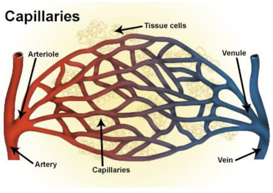
Figure 1.
Network of blood vessels (credits: Wikipedia).
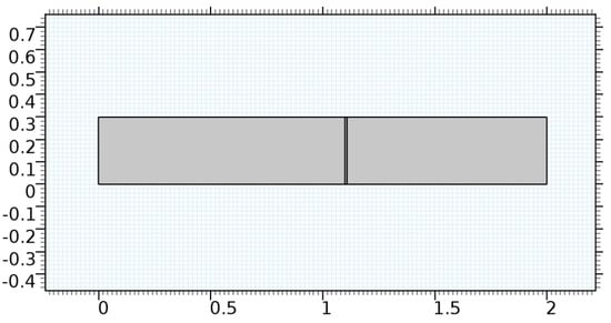
Figure 2.
Geometry of the arteriole segment.
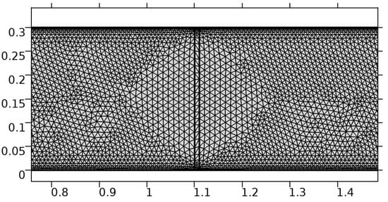
Figure 3.
Meshing near the graphene layer in an arteriole segment.
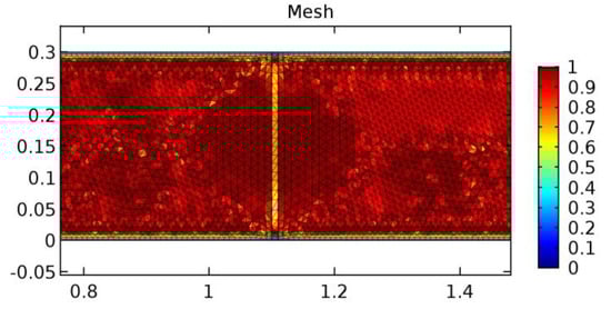
Figure 4.
Mesh quality of the fine mesh generated.
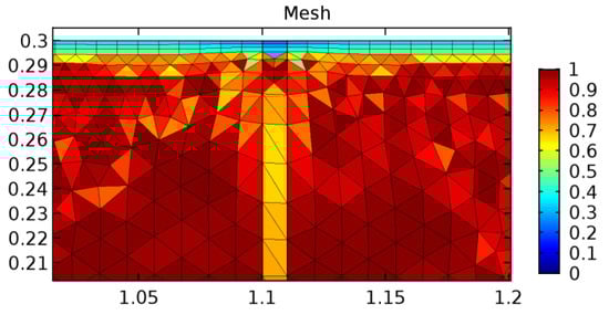
Figure 5.
Mesh quality near the graphene layer.
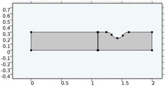
Figure 6.
Geometry of arteriole segment with stenosis in the post-graphene region.
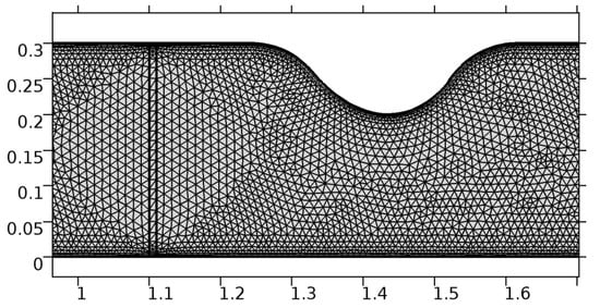
Figure 7.
Meshing near the graphene layer and the stenosis.
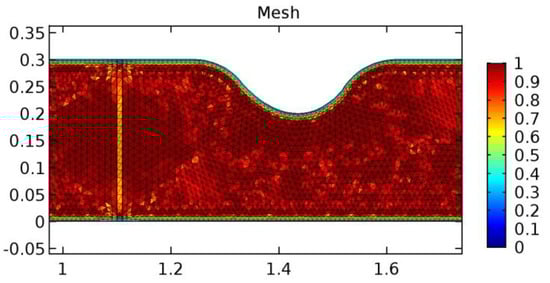
Figure 8.
Meshing near the graphene layer and stenosis.
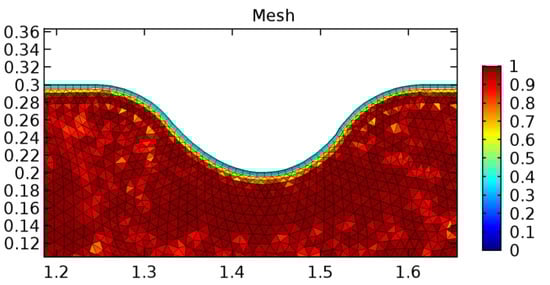
Figure 9.
Meshing near the stenosis wall.
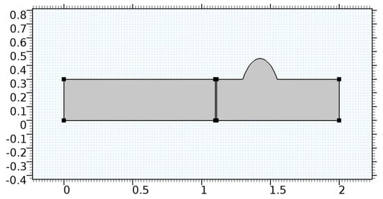
Figure 10.
Geometry of arteriole segment with aneurysmic sac in the post-graphene region.
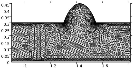
Figure 11.
Meshing near the graphene layer and the aneurysmic sac.
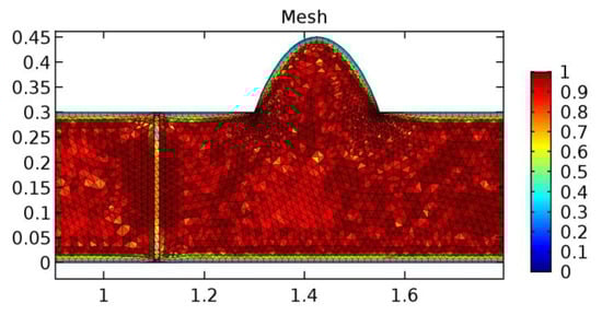
Figure 12.
Mesh quality near the graphene layer and sac.
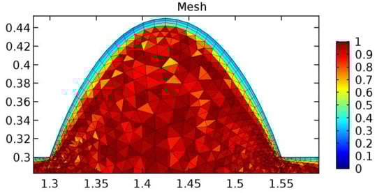
Figure 13.
Mesh quality near the sac.

Table 1.
Mesh details.
2.3. Numerical and Physical Parameters
Table 2 comprises the values of the parameters involved in the mathematical model considered to study the flow. The sources of the values of parameters are the previously published articles as well as the experimental results.
Table 2.
Numerical and physical parameter values.
The mathematical model is solved for zero-initial conditions with an inlet fluid velocity of and null outlet pressure. The analysis is made for a suitable value of porosity that allows the passage of water and blood through the graphene layer.
3. Results and Discussion
We tested the validity of the model developed for the current study on the topics covered in the research publications listed below. We want to confirm the areas with aberrant velocity, pressure, and WSS readings. For validating the model considered in the present study, we enlisted assistance from the previously published articles [40,47]. It has been noted that the results of validation obtained are in agreement with that of these articles.
We intended to explore the flow domain initially by excluding the graphene layer. Figure 14, Figure 15, Figure 16, Figure 17, Figure 18 and Figure 19 represent the flow and pressure profiles for the case of blood flow across an arteriole segment without the graphene layer. The results obtained were in good agreement with the various studies conducted previously on the blood flow across an arterial segment [39,40,41]. On comparing the velocity vector profiles of the cases without graphene and with graphene, it can be noted that inclusion of the graphene layer significantly changes the flow profile. In the case of the healthy arteriole segment, a linear flow of blood is seen, as in Figure 16. The pressure is uniformly distributed across the flow domain with the exclusion of the graphene layer in the healthy vessel, as shown in Figure 17. The inclusion of the graphene layer induces a zone of higher velocity neighboring the foot of the graphene layer (evident from Figure 20, Figure 21, Figure 22, Figure 23, Figure 24, Figure 25, Figure 26, Figure 27, Figure 28, Figure 29, Figure 30, Figure 31 and Figure 32). Figure 16 and Figure 18 depict the velocity profiles of blood flow in stenosed and aneurysmic segments, respectively. A similar zonal separation is seen due to the insertion of the graphene layer. Figure 17 and Figure 19 represent the pressure distribution without the graphene layer. As shown in Figure 33, Figure 34, Figure 35, Figure 36, Figure 37, Figure 38, Figure 39, Figure 40, Figure 41, Figure 42, Figure 43, Figure 44 and Figure 45, the pressure distribution also is majorly affected by insertion of the graphene layer. The discussion on the advantages and disadvantages of the insertion of this chemical layer is articulated in the upcoming sections of the manuscript.
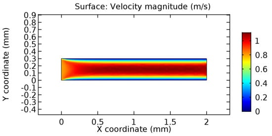
Figure 14.
Blood flow across healthy arteriole segment without graphene layer.
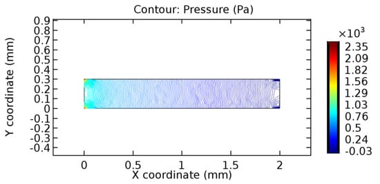
Figure 15.
Pressure profile across the healthy arteriole segment without graphene layer.
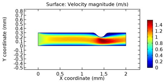
Figure 16.
Blood flow across stenosed arteriole segment without graphene layer.
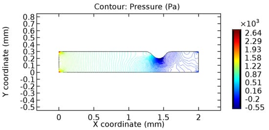
Figure 17.
Pressure profile across the stenosed arteriole segment without graphene layer.
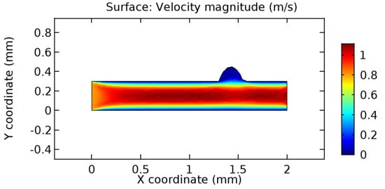
Figure 18.
Blood flow across aneurysmic arteriole segment without graphene layer.
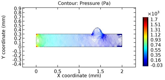
Figure 19.
Pressure profile across the aneurysmic arteriole segment without graphene layer.
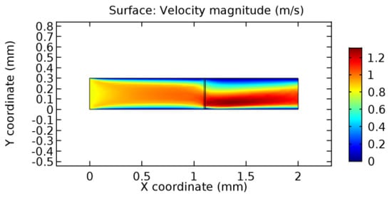
Figure 20.
Water flow across the graphene layer with 7.2% porosity (Case: Water flow).
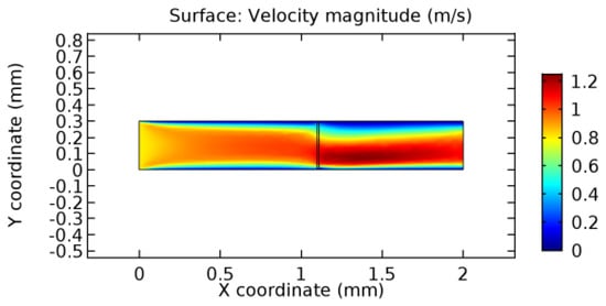
Figure 21.
Water flow across the graphene layer with 8.2% porosity (Case: Water flow).
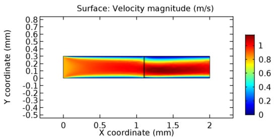
Figure 22.
Water flow across the graphene layer with 10% porosity (Case: Water flow).

Figure 23.
Blood flow across the graphene layer with 5.7% porosity (Case: Blood flow).
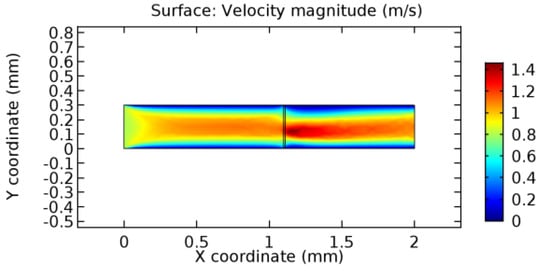
Figure 24.
Blood flow across graphene layer with 6% porosity (Case: Blood flow).
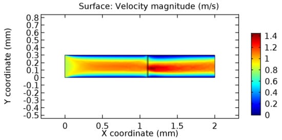
Figure 25.
Blood flow across the graphene layer with 7% porosity (Case: Blood flow).
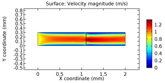
Figure 26.
Blood flow across the graphene layer with 10% porosity (Case: Blood flow).
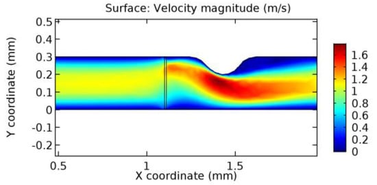
Figure 27.
Blood flow across the graphene layer with 3.5% porosity (Case: Blood flow).
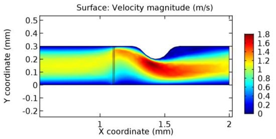
Figure 28.
Blood flow across graphene layer with 4.5% porosity (Case: Blood flow).
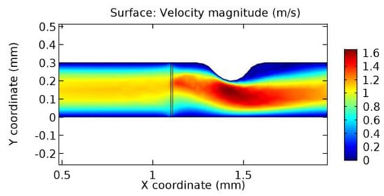
Figure 29.
Water flow across the graphene layer with 6.5% porosity (Case: Blood flow).
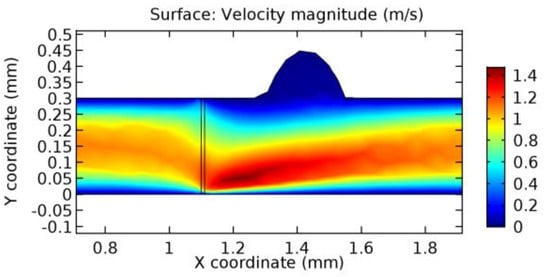
Figure 30.
Blood flow across the graphene layer with 3.5% porosity (Case: Blood flow).
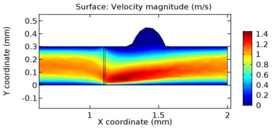
Figure 31.
Blood flow across the graphene layer with 4.5% porosity (Case: Blood flow).
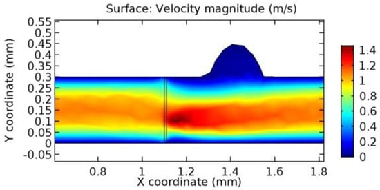
Figure 32.
Water flow across the graphene layer with 6.5% porosity (Case: Blood flow).
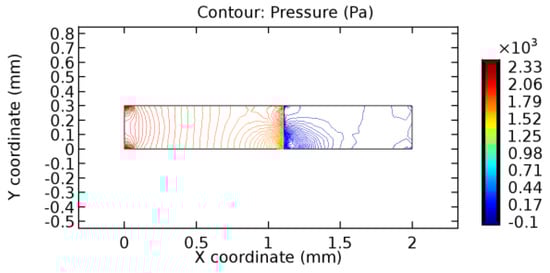
Figure 33.
Pressure distribution for graphene layer with 7.2% porosity (Case: Water flow).
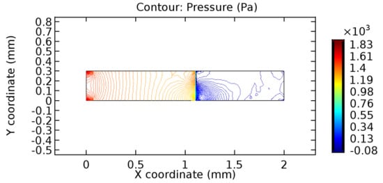
Figure 34.
Pressure distribution for graphene layer with 8.2% porosity (Case: Water flow).
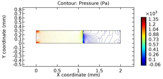
Figure 35.
Pressure distribution for graphene layer with 10% porosity (Case: Water flow).
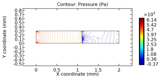
Figure 36.
Pressure distribution for graphene layer with 5.7% porosity (Case: Blood flow).
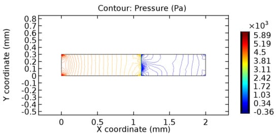
Figure 37.
Pressure distribution for graphene layer with 6% porosity (Case: Blood flow).
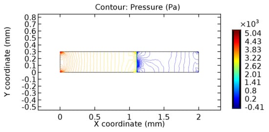
Figure 38.
Pressure distribution for graphene layer with 7% porosity (Case: Blood flow).
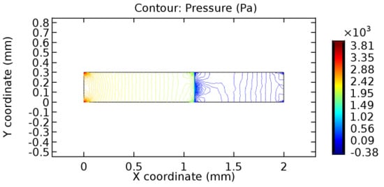
Figure 39.
Pressure distribution for graphene layer with 10% porosity (Case: Blood flow).
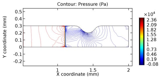
Figure 40.
Pressure distribution for graphene layer with 3.5% porosity (Case: Blood flow).
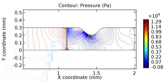
Figure 41.
Pressure distribution for graphene layer with 4.5% porosity (Case: Blood flow).
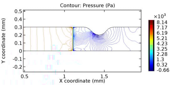
Figure 42.
Pressure distribution for graphene layer with 6.5% porosity (Case: Blood flow).
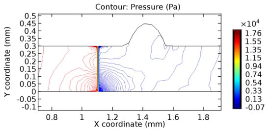
Figure 43.
Pressure distribution for graphene layer with 3.5% porosity (Case: Blood flow).
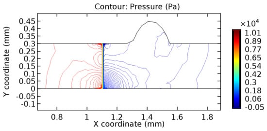
Figure 44.
Pressure distribution for graphene layer with 4.5% porosity (Case: Blood flow).
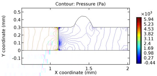
Figure 45.
Pressure distribution for graphene layer with 6.5% porosity (Case: Blood flow).
Table 3 displays the results of simulating the flow of water and blood across a graphene layer of varying porosity. The critical porosity values are shaded in red. The critical porosity value is defined as the value of porosity of a material corresponding to which the flow of a fluid is possible across the material. For water, until 7.1% porosity, there is no flow through the layer. Hence, the solutions never converged. From 7.2% porosity, flow occurs across the sheet. For blood, until 5.6% porosity, there is no flow through the layer. Hence, the solutions never converged. From 5.7% porosity, flow occurs across the sheet. The above results are taken by considering a healthy arteriole segment that is devoid of any pathologies. Similar observations were made for blood flowing across stenosed or aneurysmic arteriole segments. For water flow, it has been observed that with the increase in porosity, the number of iterations and the linear error values decrease due to the increased pore capacities. The reverse is seen to happen in the case of blood due to the complexity of blood composition. The flow of water is executed just to compare the porosity values for two different fluids with different compositions.
Table 3.
Linear error, linear residue, number of iterations, and the degrees of freedom (DoF) details.
3.1. Analysis of Flow Characteristics
3.1.1. Discussion on the Velocity Vector
Due to insertion of the graphene layer amidst the flow path, the direction of fluid flow is altered. This results in the flow being pointed towards the lower wall spot neighboring the graphene layer’s foot in the post-graphene region (PG region). This can be observed from figures on velocity profiles (Figure 20, Figure 21, Figure 22, Figure 23, Figure 24, Figure 25, Figure 26, Figure 27, Figure 28, Figure 29, Figure 30, Figure 31 and Figure 32). Due to the deviated velocity vector, the stress exerted by the flow stream on the vessel wall increases leading to the weakening of the endothelial layer of the arteriole wall. This could possibly result in spread of the existing pathology along the arteriole domain. Analysis of velocity vector questions the usage of the graphene layer in regulating stenosis or aneurysms. For blood, the velocity magnitude is more when compared to water even though the critical porosity is less for blood. In addition, for porosities greater than the critical porosity, velocity is not strongly dependent on porosity. For values below the critical porosity, velocity depends strongly on porosity and increases significantly with a small decrease in porosity. Figure 46, Figure 47, Figure 48, Figure 49, Figure 50 and Figure 51 represent the formation of recirculation zones along the flow stream. While the recirculation zones are considered, the number of recirculation zones seems to increase with the increase in porosity due to the increased flow, evident from Figure 46, Figure 47, Figure 48, Figure 49, Figure 50 and Figure 51. Again the fact of the increased number of recirculation zones goes against the purpose of our study. These recirculation zones take shelter near the foot of the graphene layer introduced.
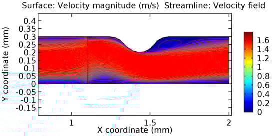
Figure 46.
Recirculation zones in blood flow through 3.5% porous graphene (Case: Blood flow).
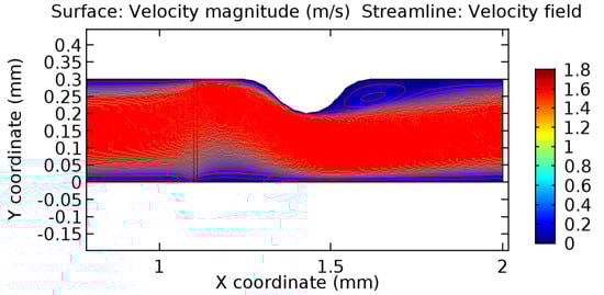
Figure 47.
Recirculation zones in blood flow through 4.5% porous graphene (Case: Blood flow).
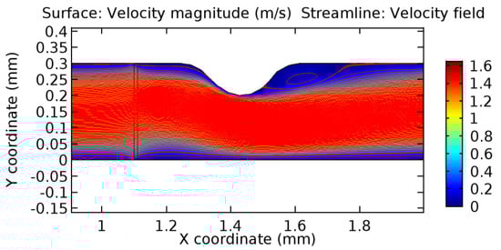
Figure 48.
Recirculation zones in blood flow through 6.5% porous graphene (Case: Blood flow).
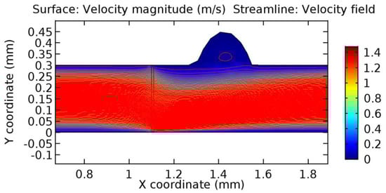
Figure 49.
Recirculation zones in blood flow through 3.5% porous graphene (Case: Blood flow).
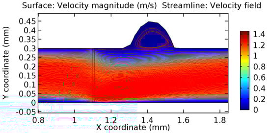
Figure 50.
Recirculation zones in blood flow through 4.5% porous graphene (Case: Blood flow).
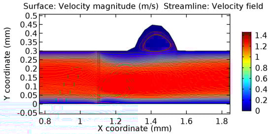
Figure 51.
Recirculation zones in blood flow through 6.5% porous graphene (Case: Blood flow).
3.1.2. Discussion on the Pressure Gradient
The biological properties of graphene tend to decrease the fluid pressure in the PG region. This causes a huge pressure gradient between the pre-and post-graphene regions in the flow domain. The high-pressure gradient causes loss of texture of the arteriole walls. This again adds a negative impact to introducing the graphene layer to the flow geometry. Figure 33, Figure 34, Figure 35, Figure 36, Figure 37, Figure 38, Figure 39, Figure 40, Figure 41, Figure 42, Figure 43, Figure 44 and Figure 45 depict the pressure distribution for various cases under study. It is noted that there has been a remarkable relaxation in the pressure magnitude due to the graphene layer. As the pressure drop is seen in the PG region, it can be noted that these regions have less chance of experiencing high flow stress over the region walls. It has been seen from the available literature [48,49] that the regions on the arterial wall experiencing a high-pressured flow are more susceptible to endothelial dysfunction. Thus, the PG region has the least potential for development of new aneurysmic sacs.
3.1.3. Discussion on the Wall Shear Stress Profile
Wall shear stress (WSS) vector illustration properties in arterioles are richly characterized by complex blood flow. Blood flow dynamics and the biology of several cardiovascular disorders are linked by WSS. WSS has attracted significant attention in a variety of research and has become the most often used indicator to link blood circulation to heart diseases. Wall shear stress profiles such as pressure profiles show a positive outcome for introducing the graphene layer to the flow field. As far as the healthy arteriole segment is considered, the WSS profiles for the lower and upper walls are different to a greater extent even though the walls are uniform. This is due to the orientation of the flow vector due to the graphene insertion. Figure 52, Figure 53, Figure 54, Figure 55, Figure 56, Figure 57, Figure 58, Figure 59, Figure 60, Figure 61, Figure 62, Figure 63, Figure 64 and Figure 65 depict the WSS profiles for water and blood for varying porosities of graphene layers. It is seen from the graphs that at the foot of the graphene sheet, a low WSS development occurs. Later in the PG region, the values gradually rise. A similar pattern is seen for blood flow across a healthy arteriole segment. From the figures, it is evident that the maximum WSS attained in each case of study decreases with the increase in the porosity of the graphene layer.
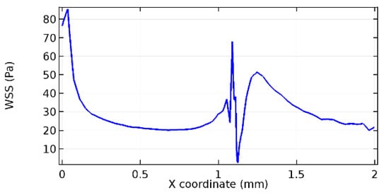
Figure 52.
Lower wall WSS for 7.2% porosity (Case: Water flow).
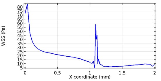
Figure 53.
Upper wall WSS for 7.2% porosity (Case: Water flow).
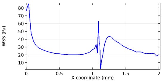
Figure 54.
Lower wall WSS for 8.2% porosity (Case: Water flow).
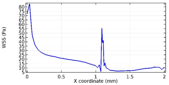
Figure 55.
Upper wall WSS for 8.2% porosity (Case: Water flow).
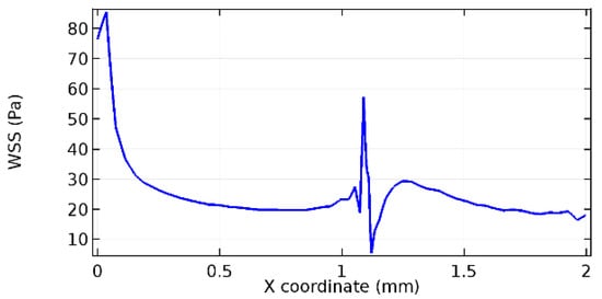
Figure 56.
Lower wall WSS for 10% porosity (Case: Water flow).
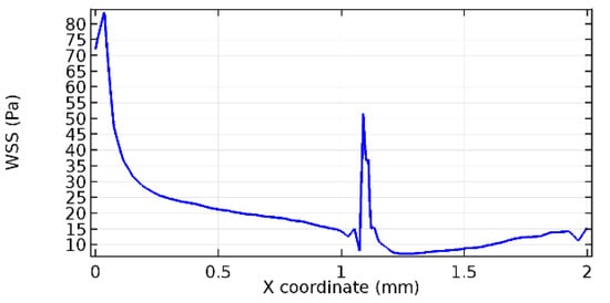
Figure 57.
Upper wall WSS for 10% porosity (Case: Blood flow).
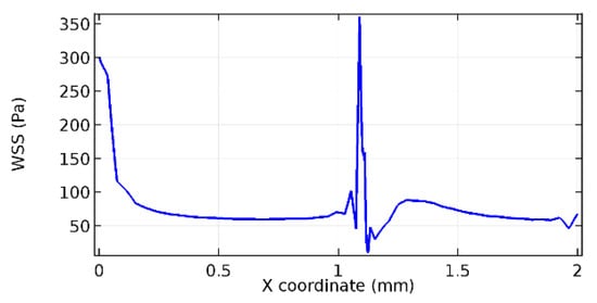
Figure 58.
Lower wall WSS for 5.7% porosity (Case: Blood flow).
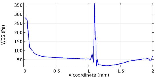
Figure 59.
Upper wall WSS for 5.7% porosity (Case: Blood flow).
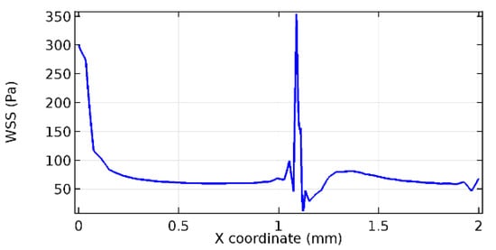
Figure 60.
Lower wall WSS for 6% porosity (Case: Blood flow).
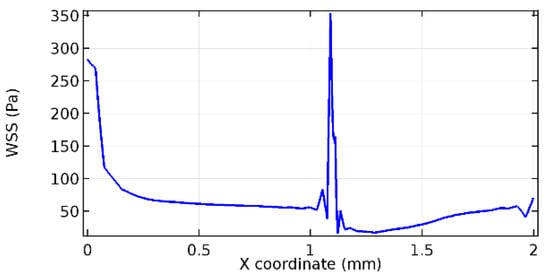
Figure 61.
Upper wall WSS for 6% porosity (Case: Blood flow).
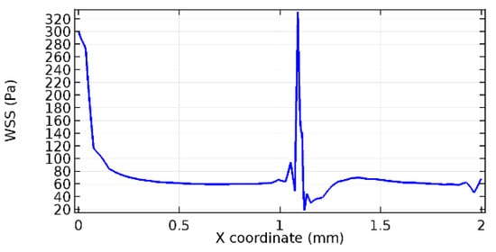
Figure 62.
Lower wall WSS for 7% porosity (Case: Blood flow).
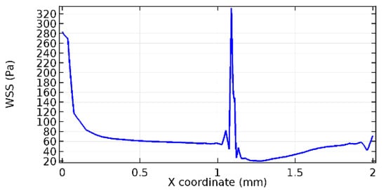
Figure 63.
Upper wall WSS for 7% porosity (Case: Blood flow).
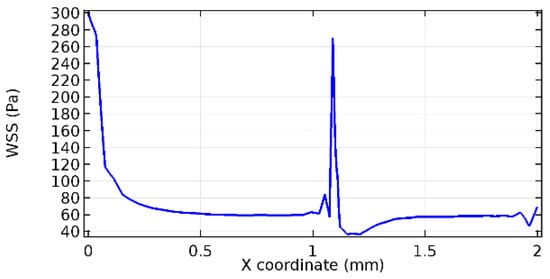
Figure 64.
Lower wall WSS for 10% porosity (Case: Blood flow).
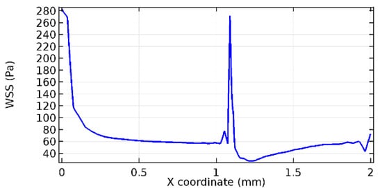
Figure 65.
Upper wall WSS for 10% porosity (Case: Blood flow).
Figure 66, Figure 67, Figure 68, Figure 69, Figure 70 and Figure 71 enclose the WSS profiles for blood in a stenosed arteriole segment. A significant difference is not seen in the WSS values along the lower wall, as there is no disturbance in the planarity of the lower wall. Again, at the foot of the graphene layer, low and oscillatory shear stress segments of graphs are seen. Graphs of Figure 72, Figure 73 and Figure 74 denote the wall shear stress profiles along the upper arteriole wall. The graph highlights the presence of nearly zero WSS regions (near the foot of the graphene layer) along the upper wall. These regions are more vulnerable to undergoing endothelial dysfunction. Figure 75, Figure 76 and Figure 77 show the shear stress pattern along the lower arteriole wall. It is noted that with the porosity progression, minimum wall shear stress attained in each of these cases is seen to decrease. It has been encountered from the clinical and theoretical literature [50,51,52] that the regions of low WSS are more prone to undergo endothelial dysfunction. The implication obvious to the above observations on WSS profiles is that the PG region is a safer zone void of chances of undergoing wall damage.
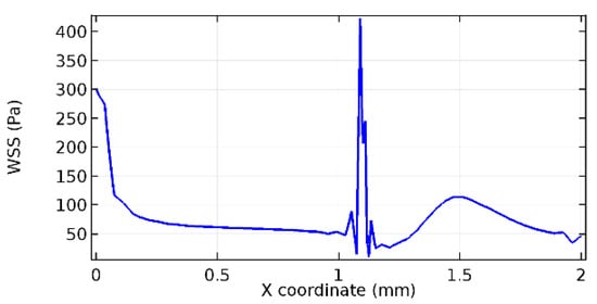
Figure 66.
Lower wall WSS for 3.5% porosity (Case: Blood flow).
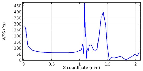
Figure 67.
Upper wall WSS for 3.5% porosity (Case: Blood flow).
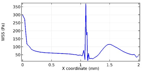
Figure 68.
Lower wall WSS for 4.5% porosity (Case: Blood flow).
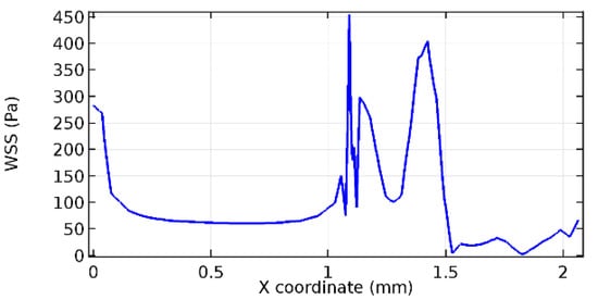
Figure 69.
Upper wall WSS for 4.5% porosity (Case: Blood flow).
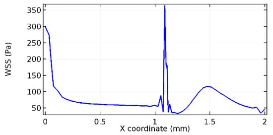
Figure 70.
Lower wall WSS for 6.5% porosity (Case: Blood flow).
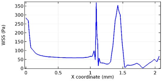
Figure 71.
Upper wall WSS for 6.5% porosity (Case: Blood flow).
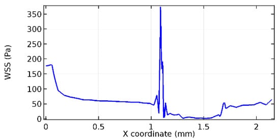
Figure 72.
Upper wall WSS for 3.5% porosity (Case: Blood flow).
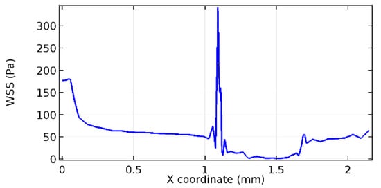
Figure 73.
Upper wall WSS for 4.5% porosity (Case: Blood flow).
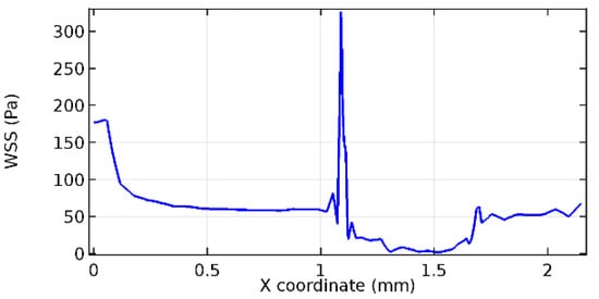
Figure 74.
Upper wall WSS for 6.5% porosity (Case: Blood flow).
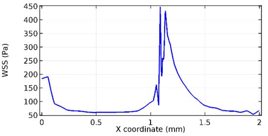
Figure 75.
Lower wall WSS for 3.5% porosity (Case: Blood flow).
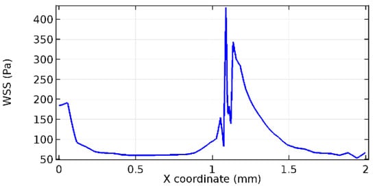
Figure 76.
Lower wall WSS for 4.5% porosity (Case: Blood flow).
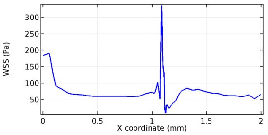
Figure 77.
Lower wall WSS for 6.5% porosity (Case: Blood flow).
4. Limitations
The current study was an observational study including a sheet of graphene permeable to fluid flows. The position of graphene was fixed, and the flow studies were taken in stationary configurations. Additionally, the angle of fixation of graphene along the flow channel was considered unaltered.
The arteriole wall is made up of three sublayers that are elastic in nature [47,48]. As the study is in the initial stages, we have considered the arterial wall to be inelastic. The inclusion of elasticity of the vessel wall would definitely improve the observational highlights.
5. Conclusions
In the current work, we investigated whether adding a graphene layer to the flow field may prevent the formation of new atherosclerotic plaque or aneurysmal sacs. It was supposed that the post-graphene zone encompassed the stenosis lump or aneurysmal sac. Through free and porous media flow topologies, the chemical characteristics of graphene were integrated with the conventional fluid flow conditions. The existence and uniqueness of the solution were examined in the governing equations. A FEM solver was used to resolve the system of partial differential equations. The following conclusions were drawn from the investigation.
- On comparing the velocity vector profiles of the cases without graphene and with graphene, it can be noted that the inclusion of the graphene layer significantly changes the flow profile.
- Inclusion of the graphene layer induced a zone of higher velocity neighboring the foot of the graphene layer.
- Velocity in the PG region dropped as porosity increased.
- A high-pressure gradient was generated due to introduction of the graphene layer to the flow field.
- The PG region has the least potential for development of new aneurysmic sacs.
- At the foot of the graphene sheet, a low WSS development occurred.
- The graphene layer introduced in the flow field harmed the flow pattern in terms of the velocity field vector. The negative impact on the flow can be due to the position of the graphene layer placed.
The present investigation, although a start to a new research domain, contributes to the existing methodologies to handle arteriole pathologies by insertion of a chemical compound layer that could bear a chance of developing the flow positively. The article contributes to the field of biomedicine through innovative key concepts of exploration such as critical porosity, the distal stand of the graphene layer across the arteriole length, and the flow parameter discussions.
Future Study Recommendations
We intend to analyze the chemical properties of graphene by conducting an extensive literature survey. The flow through the graphene layer interprets the conceptualization of the passage of blood cells through the porous media available in the graphene layer. This paradigm has evolved into several implementations using this phenomenon in the study of the circulatory system in health and illness. It enables the researchers to recreate the flow phenomena of single cells and cell suspensions in controlled, artificial settings. This principle is the basis of microfluidic technology [53,54]. By following the principles of microfluidic technology, we intend to answer the following uncertainties:
- Can the position of the graphene layer cause a remarkable difference in the flow field and flow characteristics?
- Can the angle of inclination of the graphene layer be used to obtain a positive outcome for the study?
- What effects can the elastic nature of the vessel wall have on the flow field?
- What are the possible changes in flow if the arteries are considered instead of arterioles?
- Can graphene compounds be used instead of a pure graphene layer to improve the outcomes of the study?
- Why does the graphene layer distinguish between the lower and upper arteriole walls? What factors are responsible for the differentiation?
We intend to answer the above skepticism in future research articles.
Author Contributions
Conceptualization, S.S.N. and A.M.S.; Methodology, S.S.N., N.F., F.S.A.-D. and S.A.M.A.; Software, F.S.A.-D., N.B.K. and S.A.M.A.; Validation, N.F., F.S.A.-D. and S.A.M.A.; Formal analysis, A.M.S., K.A.M.A., V.P. and M.R.G.; Investigation, S.S.N., A.M.S., K.A.M.A., V.P., M.R.G. and N.B.K.; Writing—original draft, S.S.N. and A.M.S.; Writing—review & editing, N.F., F.S.A.-D., K.A.M.A., V.P., M.R.G., N.B.K. and S.A.M.A.; Visualization, N.B.K. All authors have read and agreed to the published version of the manuscript.
Funding
The authors would like to thank the deanship of Scientific Research at Umm Al-Qura University for supporting this work by Grant code: 22UQU4310392DSR36.
Institutional Review Board Statement
Not applicable.
Informed Consent Statement
Not applicable.
Data Availability Statement
No data has been used for the current study.
Conflicts of Interest
The authors declare no conflict of interest.
Appendix A
Navier–Stokes Equation
Here, denotes the blood flow velocity, is the pressure term, represents the kinematic viscosity of blood, and is the time variable. denotes the blood flow domain (lumen) with the boundary denoted by (lower wall of the lumen).
Appendix B
Principles of Functional Analysis
Table A1.
Principles and concepts of functional analysis applied for the present study.
Table A1.
Principles and concepts of functional analysis applied for the present study.
| Sl. No. | Principle/Concept | Statement |
|---|---|---|
| 1 | Gauss formula | be a fixed domain such that . Let denote the boundary surface enclosing an area and be a vector field defined over the domain of interest. Then, |
| 2 | Caratheodory’s existence theorem | Consider the differential equation defined on the bounded domain . If the function satisfies the following conditions, then the differential equation is said to have a solution in the extended sense in a neighborhood of the initial conditions considered. The conditions are
|
| 3 | Friedrichs and Young inequalities | with diameter d. For u defined in the domain belonging to the Sobolev space
with the trace being zero over the boundary of the domain, then where is the multi-index, and is the mixed partial derivative with respect to the spatial coordinates. |
| 4 | Lower semicontinuity of a norm | is said to be lower semi-continuous if for |
| 5 | Fatou lemma | of measurable non-negative functions converges to |
| 6 | Mollifiers | Mollification is an approach for approximating a function using a smooth approximate identity. If , we define mollification using the convolution is known as the mollifier for being a nonzero positive real number. The function m is chosen from |
| 7 | Gronwall’s inequality | be continuous real-valued functions defined on is a constant. Then provided |
Appendix C
Flow through Porous Media
The porous matrix properties of the graphene layer are incorporated with the free flow equations through the equation [42]
with
where is the porosity, is the permeability, and is the mass source term.
References
- Dowlati, E.; Pasko, K.B.D.; Liu, J.; Miller, C.A.; Felbaum, D.R.; Sur, S.; Chang, J.J.; Liu, A.-H.; Armonda, R.A.; Mai, J.C. Treatment of In-Stent Stenosis Following Flow Diversion of Intracranial Aneurysms with Cilostazol and Clopidogrel. Neurointervention 2021, 16, 285–292. [Google Scholar] [CrossRef]
- Mohammad, S.; Majumdar, P. Computational Fluid Dynamics Analysis of Blood Flow Through Stented Arteries. In ASME International Mechanical Engineering Congress and Exposition; American Society of Mechanical Engineers: New York, NY, USA, 2013; Volume 56215, p. V03AT03A047. [Google Scholar]
- Prezhdo, O.V. Graphene-The Ultimate Surface Material. Surf. Sci. 2011, 605, 1607–1610. [Google Scholar] [CrossRef]
- Novoselov, K.S.; Geim, A.K.; Morozov, S.V.; Jiang, D.; Zhang, Y.; Dubonos, S.V.; Grigorieva, I.V.; Firsov, A.A. Electric field effect in atomically thin carbon films. Science 2004, 306, 666–669. [Google Scholar] [CrossRef]
- Meyer, J.C.; Geim, A.K.; Katsnelson, M.I.; Novoselov, K.S.; Booth, T.J.; Roth, S. The structure of suspended graphene sheets. Nature 2007, 446, 60–63. [Google Scholar] [CrossRef]
- Frank, I.W.; Tanenbaum, D.M.; van der Zande, A.M.; McEuen, P.L. Mechanical properties of suspended graphene sheets. J. Vac. Sci. Technol. B Microelectron. Nanometer Struct. Process. Meas. Phenom. 2007, 25, 2558–2561. [Google Scholar] [CrossRef]
- Neto, A.C.; Guinea, F.; Peres, N.M.; Novoselov, K.S.; Geim, A.K. The electronic properties of graphene. Rev. Mod. Phys. 2009, 81, 109. [Google Scholar] [CrossRef]
- Priyadarsini, S.; Mohanty, S.; Mukherjee, S.; Basu, S.; Mishra, M. Graphene and graphene oxide as nanomaterials for medicine and biology application. J. Nanostruct. Chem. 2018, 8, 123–137. [Google Scholar] [CrossRef]
- Ibrahim, A.; Klopocinska, A.; Horvat, K.; Hamid, Z.A. Graphene-Based Nanocomposites: Synthesis, Mechanical Properties, and Characterizations. Polymers 2021, 13, 2869. [Google Scholar] [CrossRef]
- Surudžić, R.; Janković, A.; Mitrić, M.; Matić, I.; Juranić, Z.D.; Živković, L.; Mišković-Stanković, V.; Rhee, K.Y.; Park, S.J.; Hui, D. The effect of graphene loading on mechanical, thermal and biological properties of poly (vinyl alcohol)/graphene nanocomposites. J. Ind. Eng. Chem. 2016, 34, 250–257. [Google Scholar] [CrossRef]
- Solanky, P.; Sharma, V.; Ghatak, K.; Kashyap, J.; Datta, D. The inherent behavior of graphene flakes in water: A molecular dynamics study. Comput. Mater. Sci. 2019, 162, 140–147. [Google Scholar] [CrossRef]
- Sanchez, V.C.; Jachak, A.; Hurt, R.H.; Kane, A.B. Biological Interactions of Graphene-Family Nanomaterials: An Interdisciplinary Review. Chem. Res. Toxicol. 2011, 25, 15–34. [Google Scholar] [CrossRef]
- Rivera-Briso, A.L.; Aachmann, F.L.; Moreno-Manzano, V.; Serrano-Aroca, Á. Graphene oxide nanosheets versus carbon nanofibers: Enhancement of physical and biological properties of poly(3-hydroxybutyrate-co-3-hydroxyvalerate) films for biomedical applications. Int. J. Biol. Macromol. 2020, 143, 1000–1008. [Google Scholar] [CrossRef]
- Thejas, R.; Naveen, C.S.; Khan, M.I.; Prasanna, G.D.; Reddy, S.; Oreijah, M.; Guedri, K.; Bafakeeh, O.T.; Jameel, M. A review on electrical and gas-sensing properties of reduced graphene oxide-metal oxide nanocomposites. Biomass Convers. Biorefin. 2022, 1–11. [Google Scholar] [CrossRef]
- Abbasi, A.; Farooq, W.; Tag-ElDin, E.S.M.; Khan, S.U.; Khan, M.I.; Guedri, K.; Elattar, S.; Waqas, M.; Galal, A.M. Heat transport exploration for hybrid nanoparticle (Cu, Fe3O4)—Based blood flow via tapered complex wavy curved channel with slip features. Micromachines 2022, 13, 1415. [Google Scholar] [CrossRef] [PubMed]
- Jahanshahi, H.; Yao, Q.; Khan, M.I.; Moroz, I. Unified neural output-constrained control for space manipulator using tan-type barrier Lyapunov function. Adv. Space Res. 2022. [Google Scholar] [CrossRef]
- Waqas, H.; Oreijah, M.; Guedri, K.; Khan, S.U.; Yang, S.; Yasmin, S.; Khan, M.I.; Bafakeeh, O.T.; Tag-ElDin, E.S.M.; Galal, A.M. Gyrotactic Motile Microorganisms Impact on Pseudoplastic Nanofluid Flow over a Moving Riga Surface with Exponential Heat Flux. Crystals 2022, 12, 1308. [Google Scholar] [CrossRef]
- Ahmed, M.F.; Zaib, A.; Ali, F.; Bafakeeh, O.T.; Tag-ElDin, E.S.M.; Guedri, K.; Elattar, S.; Khan, M.I. Numerical Computation for Gyrotactic Microorganisms in MHD Radiative Eyring–Powell Nanomaterial Flow by a Static/Moving Wedge with Darcy–Forchheimer Relation. Micromachines 2022, 13, 1768. [Google Scholar] [CrossRef] [PubMed]
- Alazzam, A.; Qasem, N.A.; Aissa, A.; Abid, M.S.; Guedri, K.; Younis, O. Natural convection characteristics of nano-encapsulated phase change materials in a rectangular wavy enclosure with heating element and under an external magnetic field. J. Energy Storage 2023, 57, 106213. [Google Scholar] [CrossRef]
- Guedri, K.; Al-Khaled, K.; Khan, S.U.; Khan, M.I.; Elattar, S.; Galal, A.M. Couple stress Darcy–Forchheimer nanofluid flow by a stretchable surface with nonuniform heat source and suction/injection effects. Int. J. Mod. Phys. B 2022, 36, 2250214. [Google Scholar] [CrossRef]
- Shoaib, M.; Naz, I.; Khan, M.I.; Raja, M.A.Z.; Zubair, G.; Nisar, K.S.; Guedri, K. Artificial intelligence knacks-based stochastic paradigm to study lie group analysis with the impact of electric field on MHD Prandtl–Eyring fluid flow system. Int. J. Mod. Phys. B 2022, 36, 2250216. [Google Scholar] [CrossRef]
- Guedri, K.; Khan, W.; Alshehri, N.A.; Mamat, M.; Jameel, M.; Xu, Y.-J.; Waqas, M.; Galal, A.M. Thermal aspects of magnetically driven micro-rotational nanofluid configured by exponential radiating surface. Case Stud. Therm. Eng. 2022, 39, 102322. [Google Scholar] [CrossRef]
- Bafakeeh, O.T.; Ahmad, B.; Noor, S.; Abbas, T.; Khan, S.U.; Khan, M.I.; Elattar, S.; Eldin, S.M.; Oreijah, M.; Guedri, K. Nonlinear Thermal Diffusion and Radiative Stagnation Point Flow of Nanofluid with Viscous Dissipation and Slip Constrains: Keller Box Framework Applications to Micromachines. Micromachines 2022, 13, 1839. [Google Scholar] [CrossRef] [PubMed]
- Ameen, F.; Altuner, E.E.; Tiri, R.N.E.; Gulbagca, F.; Aygun, A.; Sen, F.; Majrashi, N.; Orfali, R.; Dragoi, E.N. Highly active iron (II) oxide-zinc oxide nanocomposite synthesized Thymus vulgaris plant as bioreduction catalyst: Characterization, hydrogen evolution and photocatalytic degradation. Int. J. Hydrogen Energy 2022. [Google Scholar] [CrossRef]
- Al Husnain, L.; Alajlan, L.; AlKahtani, M.D.; Orfali, R.; Ameen, F. Avicennia marina endophytic fungi shows antagonism against tomato pathogenic fungi. J. Saudi Soc. Agric. Sci. 2022. [Google Scholar] [CrossRef]
- Subramaniyan, S.B.; Ameen, F.; Zakham, F.A.; Anbazhagan, V. Activity of Lipid Loaded Lectin against co-infection of Candida albicans and Staphylococcus aureus using the Zebrafish model. J. Appl. Microbiol. 2022, lxac050. [Google Scholar] [CrossRef]
- Ameen, F.; Al-Homaidan, A.A. Treatment of heavy metal–polluted sewage sludge using biochar amendments and vermistabilization. Environ. Monit. Assess. 2022, 194, 861. [Google Scholar] [CrossRef] [PubMed]
- Singaravelu, D.K.; Binjawhar, D.N.; Ameen, F.; Veerappan, A. Lectin-Fortified Cationic Copper Sulfide Nanoparticles Gain Dual Targeting Capabilities to Treat Carbapenem-Resistant Acinetobacter baumannii Infection. ACS Omega 2022, 7, 43934–43944. [Google Scholar] [CrossRef]
- Alaguprathana, M.; Poonkothai, M.; Ameen, F.; Bhat, S.A.; Mythili, R.; Sudhakar, C. Sodium hydroxide pre-treated Aspergillus flavus biomass for the removal of reactive black 5 and its toxicity evaluation. Environ. Res. 2022, 214, 113859. [Google Scholar] [CrossRef]
- Soundararajan, D.; Natarajan, L.; Trilokesh, C.; Harish, B.; Ameen, F.; Islam, M.A.; Uppuluri, K.B.; Anbazhagan, V. Isolation of exopolysaccharide, galactan from marine Vibrio sp. BPM 19 to template the synthesis of antimicrobial platinum nanocomposite. Process. Biochem. 2022, 122, 267–274. [Google Scholar] [CrossRef]
- Hassan, S.; Sabreena; Khurshid, Z.; Bhat, S.A.; Kumar, V.; Ameen, F.; Ganai, B.A. Marine bacteria and omic approaches: A novel and potential repository for bioremediation assessment. J. Appl. Microbiol. 2022, 133, 2299–2313. [Google Scholar] [CrossRef]
- Almansob, A.; Bahkali, A.H.; Ameen, F. Efficacy of Gold Nanoparticles against Drug-Resistant Nosocomial Fungal Pathogens and Their Extracellular Enzymes: Resistance Profiling towards Established Antifungal Agents. Nanomaterials 2022, 12, 814. [Google Scholar] [CrossRef] [PubMed]
- Afridi, M.S.; Ali, S.; Salam, A.; Terra, W.C.; Hafeez, A.; Sumaira; Ali, B.; AlTami, M.S.; Ameen, F.; Ercisli, S.; et al. Plant Microbiome Engineering: Hopes or Hypes. Biology 2022, 11, 1782. [Google Scholar] [CrossRef]
- Ali, F.; Rather, B.A.; Fatima, N.; Sarfraz, M.; Ullah, A.; Alharbi, K.A.M.; Dad, R. On the Topological Indices of Commuting Graphs for Finite Non-Abelian Groups. Symmetry 2022, 14, 1266. [Google Scholar] [CrossRef]
- Fatima, N.; Daniel, S. Solution of Wave Equations and Heat Equations Using HPM. In Applied Mathematics and Scientific Computing; Part of the Trends in Mathematics Book Series (TM); Springer: Berlin/Heidelberg, Germany, 2019; pp. 367–374. [Google Scholar] [CrossRef]
- Smieja, J. Advantages and pitfalls of mathematical modelling used for validation of biological hypotheses. In Proceedings of the 7th IFAC Symposium on Modelling and Control in Biomedical Systems 2009, Aalborg, Denmark, 12–14 August 2009; pp. 348–353. [Google Scholar]
- Chandran, D.; Copeland, W.; Sleight, S.; Sauro, H. Mathematical modeling and synthetic biology. Drug Discov. Today Dis. Model. 2008, 5, 299–309. [Google Scholar] [CrossRef] [PubMed]
- Silva, T.; Jäger, W.; Neuss-Radu, M.; Sequeira, A. Modeling of the early stage of atherosclerosis with emphasis on the regulation of the endothelial permeability. J. Theor. Biol. 2020, 496, 110229. [Google Scholar] [CrossRef] [PubMed]
- S, S.N.; Saha, S.; Bhattacharjee, A. A 2D FSI mathematical model of blood flow to analyze the hyper-viscous effects in atherosclerotic COVID patients. Results Eng. 2021, 12, 100275. [Google Scholar] [CrossRef]
- Narayan, S.S.; Anuradha, B.; Sunanda, S.; Puneeth, V.; Khan, M.I.; Abdullah, A.; Guedri, K.; Jameel, M. A mathematical model that describes the relation of low-density lipoprotein and oxygen concentrations in a stenosed artery. Int. J. Mod. Phys. B 2022, 36, 2250173. [Google Scholar] [CrossRef]
- Abels, H.; Daube, J.; Kraus, C. Pressure reconstruction for weak solutions of the two-phase incompressible Navier–Stokes equations with surface tension. Asymptot. Anal. 2019, 113, 51–86. [Google Scholar] [CrossRef]
- LE Bars, M.; Worster, M.G. Interfacial conditions between a pure fluid and a porous medium: Implications for binary alloy solidification. J. Fluid Mech. 2006, 550, 149–173. [Google Scholar] [CrossRef]
- Schenk, O.; Gärtner, K.; Fichtner, W.; Stricker, A. PARDISO: A high-performance serial and parallel sparse linear solver in semiconductor device simulation. Futur. Gener. Comput. Syst. 2001, 18, 69–78. [Google Scholar] [CrossRef]
- Khattab, I.S.; Bandarkar, F.; Fakhree, M.A.A.; Jouyban, A. Density, viscosity, and surface tension of water+ ethanol mixtures from 293 to 323K. Korean J. Chem. Eng. 2012, 29, 812–817. [Google Scholar] [CrossRef]
- Geim, A.K.; Novoselov, K.S. The rise of graphene. Nat. Mater. 2007, 6, 183–191. [Google Scholar] [CrossRef]
- Cilla, M.; Peña, E.; Martínez, M.A. Mathematical modelling of atheroma plaque formation and development in coronary arteries. J. R. Soc. Interface 2014, 11, 20130866. [Google Scholar] [CrossRef]
- Sherif, S.A.; Tok, O.O.; Taşköylü, Ö.; Goktekin, O.; Kilic, I.D. Coronary Artery Aneurysms: A Review of the Epidemiology, Pathophysiology, Diagnosis, and Treatment. Front. Cardiovasc. Med. 2017, 4, 24. [Google Scholar] [CrossRef]
- Chiu, J.-J.; Chien, S. Effects of Disturbed Flow on Vascular Endothelium: Pathophysiological Basis and Clinical Perspectives. Physiol. Rev. 2011, 91, 327–387. [Google Scholar] [CrossRef] [PubMed]
- Dharmashankar, K.; Widlansky, M.E. Vascular Endothelial Function and Hypertension: Insights and Directions. Curr. Hypertens. Rep. 2010, 12, 448–455. [Google Scholar] [CrossRef] [PubMed]
- S, S.N.; Saha, S. Time-dependent study of blood flow in an aneurysmic stenosed coronary artery with inelastic walls. Mater. Today Proc. 2021, 47, 4718–4724. [Google Scholar] [CrossRef]
- Kumar, A.; Hung, O.Y.; Piccinelli, M.; Eshtehardi, P.; Corban, M.T.; Sternheim, D.; Yang, B.; Lefieux, A.; Molony, D.S.; Thompson, E.W.; et al. Low Coronary Wall Shear Stress Is Associated with Severe Endothelial Dysfunction in Patients with Nonobstructive Coronary Artery Disease. JACC Cardiovasc. Interv. 2018, 11, 2072–2080. [Google Scholar] [CrossRef]
- Urschel, K.; Tauchi, M.; Achenbach, S.; Dietel, B. Investigation of Wall Shear Stress in Cardiovascular Research and in Clinical Practice—From Bench to Bedside. Int. J. Mol. Sci. 2021, 22, 5635. [Google Scholar] [CrossRef] [PubMed]
- Chen, L.; Zheng, Y.; Liu, Y.; Tian, P.; Yu, L.; Bai, L.; Zhou, F.; Yang, Y.; Cheng, Y.; Wang, F.; et al. Microfluidic-based in vitro thrombosis model for studying microplastics toxicity. Lab Chip 2022, 22, 1344–1353. [Google Scholar] [CrossRef] [PubMed]
- Chen, L.; Yu, L.; Liu, Y.; Xu, H.; Ma, L.; Tian, P.; Zhu, J.; Wang, F.; Yi, K.; Xiao, H.; et al. Space-time-regulated imaging analyzer for smart coagulation diagnosis. Cell Rep. Med. 2022, 3, 100765. [Google Scholar] [CrossRef]


Disclaimer/Publisher’s Note: The statements, opinions and data contained in all publications are solely those of the individual author(s) and contributor(s) and not of MDPI and/or the editor(s). MDPI and/or the editor(s) disclaim responsibility for any injury to people or property resulting from any ideas, methods, instructions or products referred to in the content. |
© 2023 by the authors. Licensee MDPI, Basel, Switzerland. This article is an open access article distributed under the terms and conditions of the Creative Commons Attribution (CC BY) license (https://creativecommons.org/licenses/by/4.0/).