Abstract
In full-field 3D displacement measurement, stereo digital image correlation (Stereo-DIC) has strong capabilities. However, as a result of difficulties with stereo camera calibration and surface merging, 360-deg panoramic displacement measurements remain a challenge. This paper proposes a panoramic displacement field measurement method in order to accurately measure the shape and panoramic displacement field of complex shaped objects with natural textures. The proposed method is based on the robust subset-based DIC algorithm and the well-known Zhang’s calibration method to reconstruct the 3D shape and estimate the full-field displacements of a complex surface from multi-view stereo camera pairs. The method is used in the determination of the scale factor of the 3D reconstructed surface and the stitching of multiple 3D reconstructed surfaces with the aid of the laser point cloud data of the object under test. Based on a discussion of the challenges faced by panoramic DIC, this paper details the proposed solution and describes the specific algorithms implemented. The paper tests the performance of the proposed method using an experimental system with a 360-deg six camera setup. The system was evaluated by measuring the rigid body motion of a cylindrical log sample with known 3D point cloud data. The results confirm that the proposed method is able to accurately measure the panoramic shape and full-field displacement of objects with complex morphologies.
1. Introduction
As a flexible non-contact optical-numerical technology, digital image correlation (DIC) has the characteristics of relatively straightforward data processing, easy implementation, high accuracy, and wide applicability, that have become widespread in the mechanical properties testing of materials and biological tissues [1,2,3,4,5], health monitoring of engineering structures [6,7,8], and other fields. Stereo-DIC technology combines the principles of DIC and stereophotogrammetry, which is a powerful and practical full-field optical deformation measurement technology [8,9,10]. It obtains full-field complex geometric shapes, motions, and deformations by tracking and recovering the three-dimensional shape of the deformed object in the stereo image sequence [11]. The realization of the Stereo-DIC technology requires the use of a dual-camera synchronous imaging system or a single-camera pseudo-stereo imaging system, which can simultaneously record a pair of image sequences of angled views on the specimen surface under different states. Then, the intrinsic parameters and extrinsic parameters of the dual-camera setup are calibrated according to the specific stereo camera calibration procedures [12,13]. Next, a correlation algorithm is used to match the correspondence of corresponding point pairs in the two stereo images by comparing the gray distribution of a subset of square pixels and tracking these points in a sequence of stereo images representing different states of deformation. Finally, the matched set of image points is used to reconstruct and track the 3D position of the points on the specimen surface over time by combining the calibrated parameters with stereo triangulation, and, then, determining the 3D displacement field on the specimen surface.
Despite the wide use of Stereo-DIC, its field of view is limited to the front surface of the specimen due to the occlusion of the camera’s line of sight, and it cannot measure the whole-body profile of the panoramic deformation of the sample with a complex geometric morphology. In order to extend the field of view of the deformation measurement to a panoramic view, the effective countermeasures are to adopt a multi-view imaging system composed of multiple synchronous cameras, a pseudo-multi-view imaging system composed of single camera combined with slewing ring, or a binocular imaging system assisted by mirrors. The whole-body shape and displacement measurement technique can usually be carried out according to one of the following system configurations: (i) Encircling configuration. The object to be measured is surrounded by a group of synchronous cameras deployed as an open or closed ring, with each pair of adjacent cameras having a common field of view to facilitate the integration of all cameras into a common world coordinate system [14,15]. The encircling configuration requires two or more synchronous cameras, making the measurement technique both complicated and expensive, but, even so, this configuration is still the mainstream of full-field 360-deg displacement measurements, especially for the shape and displacement measurement of large-size specimens or specimens located in industrial sites. (ii) Pseudo-encircling configuration. The configuration is also measured the object by several adjacent and intersecting views, but the difference is that the different views are captured by rotating the camera while keeping the object still or rotating the object while fixing the camera [16,17]. One serious limitation of this configuration is that it can only be used under static or quasi-static loading conditions. (iii) Discrete stereoscopic configuration. Consists of two synchronous Stereo-DIC systems with no common field of view that measure each surface of the plate or sheet specimen independently [18]. The discrete stereoscopic configuration requires four cameras to form two stereo camera pairs. On the one hand, it is similar to the encircling configuration and requires complicated calibration. On the other hand, the stereo camera pairs are independent from each other, thus, it is only suitable for dual-surface displacement field measurement of sheet specimens. (iv) Mirror-assisted configuration. A 360-deg panoramic or dual-surface view of the regular-sized specimen to be measured is obtained through specific catadioptric components, which is in the form of a planar mirror [12,19,20] or conical mirror [5,9,21]. The mirror-assisted configuration can be used for panoramic measurement, but only for specimens of comparable mirror size, and there are still challenges on shape and displacement measurement of larger objects. In addition, the entailed wide field of view required conflicts with the high spatial resolution of region of interest (ROI) required for accurate DIC measurement.
Despite the different configurations and applications for 360-deg panoramic shape and deformation measurements that can be found, the three key issues involved in achieving a multi-view panoramic setup tend to be similar and consist mainly of stereo camera calibration, spatial and temporal matching, and 3D reconstruction. The aim of stereo camera calibration is to find intrinsic parameters (defining the geometric and optical properties of the camera) and extrinsic parameters (defining the position and orientation of the camera with respect to a reference coordinate system). According to different scenes, the existing calibration algorithms can be divided into four methods: self-calibration [22,23,24,25], calibration based on 1D calibration objects [26,27,28], 2D calibration objects [29,30,31], and 3D calibration objects [32,33,34], respectively. It should be noted that the translation vector calibrated by the above calibration method is normalized and lacks scale information, which is necessary to determine the actual value of the shape and/or displacement. In this paper, with the aid of the laser point clouds, the scale factor calculation model is established by calculating the center of gravity, the centroid of the laser point cloud, and the reconstructed 3D point cloud and its corresponding relations. Spatial matching focuses on establishing a three-dimensional correspondence on two different camera views, while the aim of temporal matching is to track the pixel positions on each image sequence, both of which can be achieved by robust local feature-based image correlation algorithms [35,36]. In this paper, precise subset-based DIC following the inverse compositional Gauss–Newton algorithm and the reliability-guided displacement computation strategy is used for spatial and temporal matching; the results of spatial matching are used to establish the correspondences for extrinsic parameter estimation and to reconstruct the 3D surface profile of the measured specimen, while the results of temporal matching are used to calculate the displacement before and after deformation. A key step of panoramic shape and displacement measurement is to merge multiple local 3D surfaces (reconstructed 3D coordinates) with overlapping regions obtained based on multi-view Stereo-DIC into a single continuous merged surface. The essence of surface merging is to merge overlapping parts by removing redundant points as to obtain the complete 3D profile information of objects. The principle of surface merging is to use only the points existing in the original data. The introduction of new points not derived from actual measurements is undesirable as these points cannot be tracked in a deformed configuration and do not provide reliable displacement measurements [15]. For this reason, we propose a distance-based method for merging 3D surfaces (3D points) assisted by a laser point cloud. Based on the existing methods, this method proposes a laser point cloud data-assisted scale factor determination method and a laser point cloud data-assisted surface stitching method to achieve a true and complete shape reconstruction and full-field displacement measurement of the object under the test. We used an experimental system with a 360-deg six-camera setup (shown in Figure 1) to test the performance of the proposed method. It is important to note that when the cameras are aligned, the overlapping field of view of each group of cameras must be greater than 120° to ensure the integrity of the reconstruction.
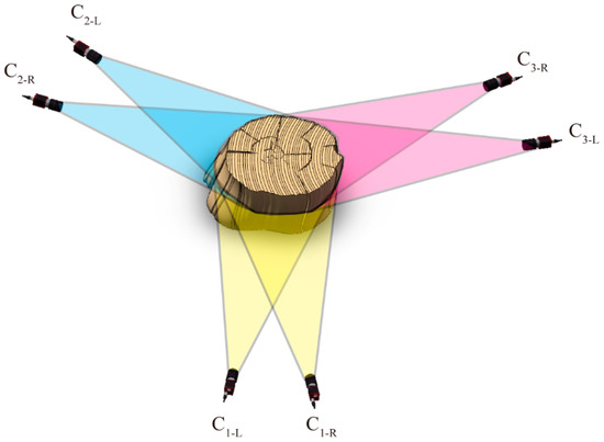
Figure 1.
360-deg six-camera measurement system schematic. A circular array of three stereo-camera pairs surrounding the object to be measured and the field of view (FOV) of each stereo camera pair exceeds 120 degrees.
The outline of this paper is as follows. Section 2 introduces the theoretical framework of the 360-deg panoramic full-field displacement measurement, including the measurement principles (Section 2.1), the intrinsic and extrinsic parameters calibration of the binocular camera pair (Section 2.2 and Section 2.3), and the three-dimensional surface profile reconstruction and displacement measurement of the specimen (Section 2.4). The experiments and discussions are presented in Section 3. Finally, we draw conclusions in Section 4.
2. Materials and Methods
2.1. Measurement Principles
The calibration of the system (for stereo triangulation) and surface merging (for combining results from multiple stereo-camera pairs) are two key issues in multi-view three-dimensional reconstruction and deformation measurements [15]. As a first step, the proposed method uses a checkerboard planar calibration target (Zhang’s method) to obtain the intrinsic parameters of each camera. The external parameters of each stereo camera pair are then calibrated in a common field of view (FOV) of both cameras using specimen surfaces with natural textures or sprayed patches. Specifically, the robust subset-based DIC method accurately detects a point match between the two images of the test specimen. The essential matrix can be determined by combining the extrinsic parameters with the determined intrinsic parameters. By decomposing the essential matrix, the available extrinsic parameters between stereo camera pairs without scale information can be obtained. Based on the above premise, the three-dimensional coordinate point cloud data for the physical three-dimensional points of the specimen without the scale information can be calculated from the pair of images by triangulation. Next, the iterative closest point (ICP) algorithm is used to match the whole three-dimensional laser-point cloud data of the specimen with the local point cloud data reconstructed by triangulation to obtain the true scale information, the rotation matrix, and the translation vector relative to the laser point cloud, which are used to determine the local three-dimensional reconstruction surface of the specimen. The local point clouds obtained from stereo-camera pairs are independent, disconnected from each other, and may overlap locally. Then, the proposed distance-based three-dimensional point merging method is used to remove redundant three-dimensional points and construct a continuous merged three-dimensional surface. Using the same intrinsic and extrinsic parameters of cameras and merging method, the three-dimensional surface of the deformed specimen is constructed in combination with the deformed point cloud data obtained from the DIC. To estimate the full-field displacements, all measurement points at their initial state are subtracted from the measurement points at their deformed state.
2.2. Planar Target-Based IntrinsicPparameters Determination
For a three-dimensional point in the world coordinate system, the coordinates of the corresponding pixel point in the image coordinate system are given by . Assuming the camera is zero-skew, by mapping the three-dimensional point corresponding to into the homogeneous coordinate system, the undistorted coordinates of with its the components and are determined.
where can be expressed in terms of the focal length and the principle point as . The matrix and the vector are the rigid-body rotation matrix and translation vector from the world coordinate system of P to the camera coordinate system, respectively, and the operator maps a 3-vector to a 2-vector .
The lens distortions, both radial and tangential, typically deteriorate imaging. Since tangential distortion, which can lead to unstable optimization, is negligible for modern camera lenses [31], we only consider the parametric radial distortion model, which can be written as follows:
where , are the coefficients of radial distortion. With the model , the distorted image coordinates with its components, and in the normalized image coordinate frame can be given by:
The basic linear equations for the banded block matrix used to determine the radial distortion model can be reformulated in a component-wise manner by Equation (3) as follows:
For calibration, we use a checkerboard planar calibration target with control points in different poses. Based on Equation (4), a system of linear equations are established. The closed-form solutions for the radial distortion coefficients and can be solved by superimposing them with the linear least square method.
The control point on the calibration target is denoted as , and and (1 ≤ j ≤ N) are denoted as the rotation matrix and translation vector corresponding to the pose of the target with respect to the camera, respectively. Then, the reprojection errors of the control point in the normalized image domain can be expressed as:
where denotes the normalized undistorted coordinates of from the jth calibration pose, which can be expressed as . Considering all control points and all target poses, a nonlinear problem is eventually obtained by using norm as a loss metric of the reprojection errors as follows:
By minimizing above nonlinear model, the optimal intrinsic parameters can be obtained. For intrinsic parameters, they are independent parameters for each camera and can, therefore, be assumed to be unchanged through mechanical fixation [37]. The relevant algorithm is given in Algorithm 1.
| Algorithm 1. Determining intrinsic parameters from planar calibration target. |
| Input: images of the target under different positions by moving target: . |
| Output: intrinsic parameters: . Initially intrinsic parameters estimation 1. Detect the control points in a series of checkerboard images with different positions. 2. Estimate the intrinsic parameters ) using the closed-form solution using Zhang’s classical calibration method [38]. 3. Estimate the radial distortion coefficients ) by linear least-squares using Equation (4). Refine intrinsic parameters Refine all intrinsic parameters by minimizing Equation (6). |
There is one thing to note here. Lens distortion cannot be ignored in practical application scenarios. Therefore, before calculating the essential matrix and applying the bundle adjustment method in the following steps, the coordinates of the corresponding points should be corrected according to the distortion coefficients obtained through calibration [24].
2.3. Epipolar Geometry-Based Extrinsic Parameters Determination
Once the intrinsic parameters of each camera in a binocular stereo camera system are calibrated, the determination of the extrinsic parameters of the binocular stereo camera system becomes a matter of positional estimation, i.e., estimating the rotation matrix and translation vector between two cameras from a set of image point correspondences between two cameras.
2.3.1. Stereo Point Matching Registration
Based on the robust subset-based digital image correlation method, the stereo point correspondences between two distinct camera views are realized, through which a set of accurate point matches can be registered for subsequent extrinsic parameters determination. Firstly, the specimen is decorated with a stable, random, high-contrast scatter pattern, or the inherent natural texture of the test specimen is exploited and captured by stereo-camera pairs. Secondly, in the image on the left, a ROI is selected, consisting of a grid of equidistant computed points that correspond to the sample area visible from both camera views. Then, based on the selected subset size and the calculated grid points within the ROI, the corresponding points are detected on the right image using the subset-based DIC. Briefly, for the initial computed points, called seed points, a square reference subset centered on them is selected and, then, iteratively minimized using the least squares correlation criterion as the correlation function to match them to the target subset of the right-hand image. A first-order shape function is used to describe the transformation of the subset, an inverse synthetic Gauss–Newton method (IC-GN) is used as a non-linear optimizer, and a reliability-oriented approach is used to transfer the calculation to the ROI to achieve a series of image point correspondences between the left and right cameras. The detailed principles and step-by-step implementation of the algorithm are presented in [39,40].
2.3.2. Five-Point Algorithm-Based Essential Matrix Estimation
The projective geometry between the left and right views of a stereo camera system is the epipolar geometry. The epipolar geometry can be represented by the essential matrix:
where is the essential matrix connecting the pose relations between the two cameras through points in space, and are the normalized image coordinates of the corresponding points in the left and right images of the stereo camera pair matched by DIC. For a pair of cameras whose intrinsic parameters have been calibrated, the essential matrix takes the form
where is defined as a skew-symmetric matrix of 3-vector, while and represent the rotation matrix and translation vector between the left and right cameras, respectively.
Since the essential matrix has two equal and non-zero singular values, this leads to the following important three-dimensional constraints on the essential matrix:
The five-point algorithm is used to compute the reliable essential matrix through the corresponding points. For a detailed implementation process one can refer to the classical work in the literature [41] and easy-to-use, effective open-source codes [42]. It is important to note that due to the scale equivalence of the essential matrix, it can only reflect the relative position relationship independent of the specific scale and cannot describe the absolute position relationship between two cameras.
2.3.3. SVD Based Extrinsic Parameters Initialization
For any matrix, it is always possible to decompose it into the product of a unitary matrix , a diagonal matrix and a transpose of another unitary matrix . As soon as the essential matrix is obtained, the singular value decomposition (SVD) of the essential matrix is expressed as:
The and describing the rigid-body transformation from the left camera to the right camera can be obtained as follows:
where , is the last column of the unitary matrix .
From geometric considerations, there are four possibilities for the combination of and . The positive depth constraint [43] is used to eliminate the redundant solutions from all possible solutions and extract the true solution. It retrieves a point in the world coordinate system using these four possible extrinsic matrices and selects the reconstructed world point located in front of the two cameras, i.e., the point should be in the positive direction of the z-axis [44].
2.3.4. Bundle Adjustment Based Extrinsic Parameters Refinement
After decomposition of the essential matrix, an initial estimation of the camera pose can be obtained. The epipolar constraint in Equation (8) cannot be fully satisfied due to the presence of image noise and interference in the stereo correspondence and camera parameters estimation. Therefore, the bundle adjustment method is used to optimize the extrinsic parameters of the cameras. The Euclidean distance between the reprojection point and the original coordinate point is the reprojection error. By minimizing this reprojection error, the optimal solution of the extrinsic parameters of camera can be obtained. The solution equation for bundle adjustment method can be expressed as:
where is the three-dimensional coordinate in the actual three-dimensional frame. The corresponding reprojected 2D points in the two image planes can be expressed as . is original the pixel coordinates of the ith point in image . When equals 1, it means left camera, and when equals 2, it means right camera. is the intrinsic matrix of camera pairs, and , and are the rotation matrix and translation vector with respect to the left camera, respectively. For the left camera, , we have and .
The optimization method used here is the Levenberg–Marquardt algorithm. Through the bundle adjustment method, the optimal extrinsic parameters of each camera pair can be obtained. It should be noted that the translation vector calculated by the above method is the normalized values, where . In Algorithm 2, the relevant algorithm for extracting extrinsic parameters is given step by step.
| Algorithm 2. Determining extrinsic parameters from matched points. |
| Input: normalized image coordinate: and . |
| Output: extrinsic parameters: and . Initially extrinsic parameters estimation 1. Estimate the essential matrix by using the five-point algorithm. 2. Based on the SVD of , calculate and using Equations (10) and (11). Refine extrinsic parameters Refine extrinsic parameters by Equation (12). |
2.3.5. Point Registration Based Scale Information Determination
Scale information is a key factor in determining the actual shape and actual displacement values and can, in principle, be determined in three ways: (1) the physical distance between two known points on the specimen, (2) the known shape of the specimen, and (3) the known displacement of the specimen. In order to calibrate the scale information, the following method is proposed based on laser scanning point clouds and ICP algorithms [45]. The three-dimensional point cloud contains rich geometric information in the spatial domain. According to the invariability of the relative position of the center of gravity and the centroid of the point cloud in the rigid body transformation, the distance ratio between the center of gravity and the centroid of the point cloud at different scales is defined as the scale factor, and the scale information model is established. Combined with the ICP algorithm, the minimum registration error function is defined to refine the scale information. Details are given below.
Firstly, filtering the point cloud data. The original-scale three-dimensional point cloud data of the test specimen and the normalized-scale three-dimensional reconstructed point cloud data were obtained by laser scanning equipment and the aforementioned method, respectively. The original-scale point cloud data obtained by laser scanning is dense, thus, it needs to be filtered to reduce the amount of point cloud data and improve the efficiency of alignment. The normalized-scale point cloud data obtained by using above three-dimensional reconstruction will contain noise and outliers, which will affect the accuracy of the calculation of center of centroid and center of gravity as well as the final alignment results, thus, the normalized-scale point cloud data are filtered to reduce or even eliminate the influence of noise and outliers.
Next, establishing a scale factor calculation model. If the center of gravity and the centroid of the original-scale point cloud data and normalized-scale point cloud data are denoted as , and and , respectively, and point , , and can be expressed as , , and . Where and are the points on point cloud data and , respectively. and are the number of points in the point cloud data, and is the centroid factor, satisfying . The scale factor has form of
where function defines the Euclidean distance between two points. The scale factor calculated by Equation (13) is taken as the initial value, the normalized-scale point cloud is scaled up equally to obtained the point cloud , which is used for the subsequent iterative optimization of scale factor.
Thirdly, refining the scale factor. The point cloud is very close to the original-scale point cloud. In this step, the accuracy of the scale factor is improved further through the ICP iterative calculating method. For each point in the normalized-scale point cloud data , the pairwise point is searched by taking the closest point of Euclidean distance on the original-scale point cloud data as the corresponding relationship. According to the corresponding relationship, the objective function is formulated here based on least square criterion as follows:
Equation (14) contains the scale factor , the rotation matrix , and the translation vector , which are substituted into the ICP algorithm to calculate the alignment error and compared with the set threshold value of alignment error, scale factor, rotation matrix, and translation vector. These are refined when the termination condition is not satisfied, and the iterative calculation is carried out to finally obtain the scale factor at the minimum alignment error. The relevant algorithm steps are presented in Algorithm 3. It should be pointed out that the rigid transformation matrices and between the reconstructed local three-dimensional points and the laser point cloud are also synchronously optimized in the process of the iterative optimization of scale factors, which are used for registration between the reconstructed local three-dimensional points and the laser point cloud. This registration process is necessary because the registration results are to be used for subsequent overlapping three-dimensional point mergers.
| Algorithm 3. Determining scale factor from point cloud registration. |
| Input: original-scale point cloud: , normalized-scale point cloud: , alignment error threshold: . |
| Output: scale factor: , rotation matrix: , translation vector: . Initially scale factor estimation 1. Calculate center of gravity and the centroid of and , respectively. 2. Calculate the initial value of according to Equation (13). Refine scale factor, rotation matrix and translation vector 1. Enlarge the normalized-scale point cloud according to the initial value of . 2. Refine scale factor, rotation matrix and translation vector by minimizing Equation (14). |
2.4. Three-Dimensional Shape Reconstruction and Full-Field Displacements Determination
Once the intrinsic and extrinsic parameters and scale factor of each stereo camera pair have been calibrated, the local 3D shape (reconstructed 3D coordinates) of the test specimen is reconstructed from the stereo correspondences by using a linear triangulation algorithm [46,47]. The local three-dimensional shapes obtained by each camera are independent and have no relationship with each other, but there is local overlap. In order to construct a continuous merged surface, the overlap between the three-dimensional points needs to be resolved and the adjacent three-dimensional points stitched together. In order to solve the overlapping problem, an algorithm is proposed. Based on the registration results of the reconstructed local three-dimensional points and laser point cloud, the algorithm starts from the boundary of the overlap regions, calculates the distance between the overlap points and the laser point cloud in the overlap regions, and removes the points with large distance to the laser point cloud until the overlap regions is spliced into a single continuous surface, as shown in Figure 2. The coordinates of the removed points are recorded for redundancy removal and merging of the overlapped three-dimensional points after deformation. Using the same intrinsic and extrinsic parameters of cameras and merging method, combined with the deformed point cloud data obtained by DIC, the three-dimensional surface of the deformed specimen is constructed. The three-dimensional displacement fields of the test specimen are finally estimated by subtracting the three-dimensional coordinates of all measurement points at initial state from those of deformed states. The relevant algorithm steps are presented in Algorithm 4.
| Algorithm 4 Determining full-field displacements from three-dimensional shape reconstruction. |
| Input: correspondence points of each camera pair: intrinsic parameters of each camera: , extrinsic parameters of each camera pair: , , . |
| Output: full-field displacement component: . Local 3D shape construction Reconstruct local 3D coordinates based linear triangulation algorithm. Global 3D shape merging Merge a complete 3D shape in the current state based on the proposed distance-based three-dimensional point merging method with the aid of laser point cloud. Panoramic displacement fields measurement Extract the panoramic displacements from the 3D position of the points under different states. |
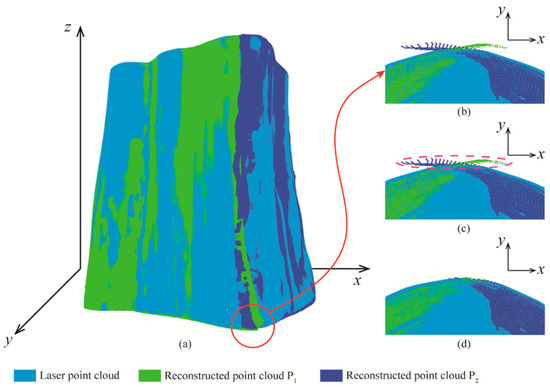
Figure 2.
Point cloud merging example. (a) A reconstructed surface with partially overlapping. (b) The elevation view of the red part, with local overlap of the data. (c) Identifies the overlapping areas and finds points within the overlapping areas which are far from the laser point cloud. (d) The result after removing the overlapping points.
3. Experiments and Discussions
First of all, an experimental setup for measuring the whole-body shape and displacement was established by taking the log as the specimen. Then, the effectiveness and accuracy of the proposed method were verified by two validation experiments, including three-dimensional shape reconstruction and translation of a log. Finally, the measurement results of the whole-body shape and displacement field of the log were presented and discussed.
3.1. Experimental Setup
A 360-deg panoramic camera setup consisting of three sets of binocular cameras was constructed, as shown in Figure 3. The six cameras (industrial camera 130SM, with an MX 1.3-megapixel 5.270 × 3.960 mm2 CMOS sensor) were placed coaxially to form three stereo camera pairs with field of view greater than 120° to ensure that the field of view between adjacent camera pairs overlaps to achieve the panoramic three-dimensional reconstruction. At the same time, it could provide an acceptable distortion level between each image pair to ensure accurate displacement measurement. In order to effectively suppress the inhomogeneous fluctuation of ambient light and chromatic aberration, three monochromatic blue LED light sources of 450–455 nm were employed. The object to be measured was placed on a translational stage in the center of the panoramic camera setup, where it could be evenly illuminated by blue LED light sources. All cameras were connected via an Ethernet hub and were controlled synchronously using a PC. A log with a height of about 320 mm and a diameter of about 260 mm with a natural texture on the surface was selected for the test sample, and the three-dimensional point cloud data of the log was obtained by using a handheld three-dimensional laser scanner (SIMSCAN, scanning accuracy 0.02 mm). The test sample and the scanning results are shown in Figure 4.
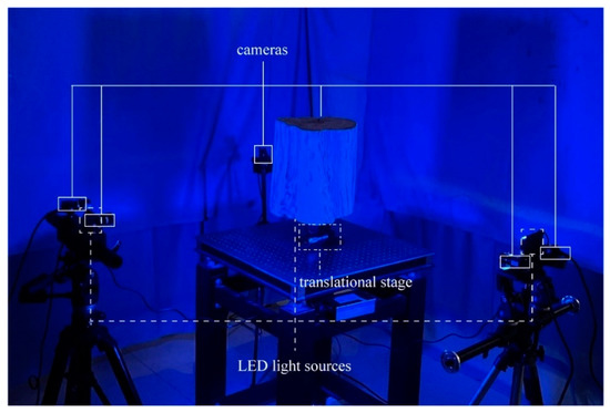
Figure 3.
A 360-deg panoramic experimental setup.
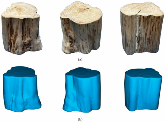
Figure 4.
The test specimen and the scanning point cloud of the test specimen. (a) The test specimen at different viewpoints. (b) The scanning point cloud of the same viewpoints in (a).
3.2. Evaluation of Separate Camera Parameters Calibration Method
3.2.1. Intrinsic Parameter Details
The intrinsic parameters of each of the six cameras (which constitute three stereo camera pairs) were determined by using Zhang’s famous method [38], respectively. In this study, the calibration target we used was a flat checkerboard with 10×10 squares and 25 mm spacing, and 18 pairs of calibration images were captured by each camera. The results of intrinsic parameters of the six cameras are listed in Table 1. In the table, and denote the focal lengths, here expressed as the pixel value. and denote the coordinates of principal points of the camera. and denote the radial distortion coefficients of the lens.

Table 1.
Intrinsic parameters determined by planar target.
3.2.2. Extrinsic Parameters Details
In order to estimate the extrinsic parameters of each stereo camera pair in the experimental setup as shown in Figure 3, three sets of images were acquired with three stereo camera pairs from a scene containing the log with the natural texture on the surface. The regions of interest were selected and a number of feature points (approximately 400,000 feature points per camera pair in this paper) were determined in the reference images of the left camera of each set of stereo camera pair, and the distortion parameters calculated in the previous step were used to correct the distortion on the detected image control points. The registrations were established in the current image of the right camera according to the method in Section 2.3.1. By employing the extrinsic parameters estimation method given in Algorithm 2, three sets of optimal relative rotations (obtained by the Rodriguez transform of the rotation matrix) and normalized translation vectors were obtained, respectively, and are listed in Table 2, where the reprojection errors are 0.08 pixels, 0.06 pixels, and 0.12 pixels, respectively, which are very low error levels.
Table 2.
Extrinsic parameters determined by proposed method.
3.2.3. Scale Factor Details
Although the translation vector calculated by the above method is the result of normalization, it can be restored to its original dimension so long as there is a known dimension in the view. In this study, the laser point cloud data of the log specimen was used as the know dimensions in the view, and Algorithm 3 was used to calculate the scale factor of each stereo camera pair. Through iterations of the ICP algorithm, not only the optimal scale factor for each stereo camera pair was obtained, but also the rotation matrix and translation vector of each reconstructed real scale point cloud with respect to the laser point cloud are obtained simultaneously, which are listed in Table 3. In this step, each pair of corresponding image points was converted from image coordinates to three-dimensional coordinates by a linear triangulation algorithm [46] using the camera-related calibration parameters. The local three-dimensional shape of the log was optimized to the real scale during the ICP iteration, as shown in Figure 5. The three local reconstructed shapes contain all the information of the 360-deg contour features of the log. Although the edges were defective, there were overlapping regions in the edges of the three reconstructed shapes, and an overlap was observed between the data. In order to quantitatively assess the accuracy of the three-dimensional reconstruction results based on reliable scale information, the reconstructed three-dimensional points were overlaid on the reference position of the laser point cloud. The root mean square error (RMSE) between the original laser point cloud and the constructed point cloud represents the stereo calibration error. The RMSEs in the three reconstructions were 0.61 mm, 0.75 mm, and 0.93 mm, respectively, indicating good reconstruction results.
Table 3.
Scale factor, relative rotation and translation vector determined in the measurement.
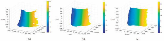
Figure 5.
Real scale three-dimensional reconstruction results. (a–c) are the reconstructed surfaces of camera pairs C1, C2 and C3, respectively. All units in the diagram are in mm.
3.3. 3D Displacement Measurement of Log Specimen
The next set of validation experiments involved the same log, whose surfaces were imaged using a set-up of 360-deg cameras and analyzed using panoramic DIC. The experimental system was evaluated by analyzing the merging errors of adjacent camera pairs, the accuracy of the reconstructed shape, the panoramic displacement errors, and the performance of the panoramic DIC algorithm.
3.3.1. Merging Error
By reconstructing the visible part of two adjacent stereo camera pairs, the merging error of different stereo cameras on the reconstructed local surface was evaluated. The overlap of reconstructed three-dimensional point clouds of two adjacent stereo camera pairs should be theoretically the same. Therefore, the Euclidean distance between the reconstructed overlapping points was represented by the merging error by two adjacent stereo cameras. In this study, three groups of overlapping three-dimensional point clouds were selected, and the average combined error was calculated as 0.5 mm.
3.3.2. 3D Reconstruction Error
In order to ensure the measured three-dimensional displacement field is credible, the correctness of the reconstructed panoramic three-dimensional profile of the log with the known three-dimensional laser point clouds was first investigated. This was achieved by matching the measured log surface topography with the wood surface topography obtained by laser scanning using the ICP algorithm. To do this, the measured three-dimensional point cloud of the logs was mapped onto the laser point cloud data and the Euclidean distance between each measured three-dimensional point and the corresponding point on the laser point cloud data was calculated to obtain the error map shown in Figure 6. As can be seen from Figure 6, the measured three-dimensional shape of the logs is identical to the true shape, with an average error of less than 2 mm. The average error for each single surface is shown in Table 4. The validation results prove the correctness of the proposed measurement principle. As the three-dimensional displacement calculation is strongly dependent on the reliability of the three-dimensional shape reconstruction, validation from a geometrical point of view is reasonable and necessary. Combined with the validation results of camera calibration and surface merging, the proposed panoramic displacement measurement system can be considered reliable and can provide correct and reliable 360-deg three-dimensional displacement measurements for complex shaped objects.
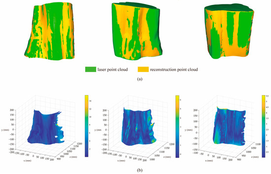
Figure 6.
3D reconstruction result and error. (a) reconstruction point cloud matched with the laser point cloud. (b) the corresponding point distance error maps, the units in the diagram are in mm.
Table 4.
The average error for each single surface.
3.3.3. 3D Displacement Error
The linear translation stage was used to translate the log specimen with the natural texture in five-step increments of 2 mm, and the displacement measured by the panoramic DIC method was compared with the displacement applied by the translation stage to calculate the displacement error. To verify the accuracy of the displacement measurement by the panoramic DIC method, based on the aforementioned verification, the displacement field of the translation experiment was retrieved and analyzed, as shown in Figure 7. In Figure 7a, The horizontal coordinates are the applied displacements and the vertical coordinates are the measured displacements by the panoramic DIC method, the measured displacements are averaged and plotted against the applied displacements, which, at first glance, almost coincide with the applied displacements. Subsequently, the errors of the displacement, including the mean error and standard deviation, are obtained, as shown in Figure 7b. In Figure 7b, the horizontal coordinates are the same as in Figure 7a. Quantitatively, for the translation experiment, the maximum absolute mean bias and maximum standard deviation were 0.0716 mm and 0.1066 mm, respectively. Both the mean bias and standard deviation in the translation experiment were small, as with the regular Stereo-DIC error, which provide a good validation of the displacement measurement capability of the panoramic DIC method.
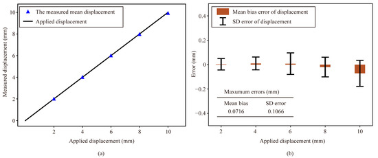
Figure 7.
Displacement measurement results. (a) Mean displacement for translation tests versus the pre-applied displacements; (b) mean bias error and standard deviation error of the measured displacements.
4. Conclusions
This paper presents a panoramic full-field three-dimensional shape and displacement measurement method for measuring complex shaped objects, assisted by laser point cloud data. A measurement system containing three simultaneous Stereo-DIC configurations is established based on an encircling configuration that captures clear images of cylindrical specimens from multiple views at fixed angular positions. In order to obtain correct and reliable measurements, key algorithms are proposed, including separate calibrations of intrinsic and extrinsic parameters, laser point cloud-assisted scale factor calibrations, and panoramic three-dimensional surface merging, which make up for some shortcomings of the camera calibration and surface merging methods commonly used in multi-view three-dimensional DIC measurements. Through a series of verification tests, the feasibility of the panoramic DIC system based on the above algorithms for panoramic shape and displacement measurements is demonstrated, and it is shown that the system can accurately and reliably measure complex 360-deg shape and three-dimensional displacement fields. A major advantage of the proposed panoramic measurement method is that only a simple calibration process is required with the aid of laser point cloud data and the surface texture of the object being measured, even when a large number of cameras are used. The measurement errors associated with the entire 360-deg panoramic DIC system were evaluated by measuring the merging errors, three-dimensional reconstruction errors, and displacement errors of the log with the natural texture. The local shape measurement error was less than 1 mm, the combined error was about 0.5 mm, the whole three-dimensional reconstruction error was less than 2 mm, and the displacement error was less than 0.1 mm. In our case, this is accurate enough to be acceptable in most applications involving complex shape displacement measurements of large dimensions.
Author Contributions
Conceptualization, Y.L.; methodology, Y.L. and D.Z.; software, J.Z. (Jianzhong Zhang); validation, D.Z. and J.Z. (Jian Zhao); formal analysis, Y.L.; investigation, Y.L.; resources, D.Z.; data curation, Y.L.; writing—original draft preparation, Y.L.; writing—review and editing, Y.L., D.Z., X.M. and J.Z. (Jian Zhao); project administration, J.Z. (Jian Zhao); funding acquisition, J.Z (Jian Zhao). All authors have read and agreed to the published version of the manuscript.
Funding
This research was funded by the Fundamental Research Funds for the Central Universities, grant number 2021ZY67.
Institutional Review Board Statement
Not applicable.
Informed Consent Statement
Not applicable.
Data Availability Statement
The data that support the findings of this study are available on request from the corresponding author, upon reasonable request.
Conflicts of Interest
The authors declare no conflict of interest.
References
- Merezhko, M.S.; Merezhko, D.A.; Rofman, O.V.; Dikov, A.S.; Maksimkin, O.P.; Short, M.P. Macro-Scale strain localization in highly irradiated stainless steel investigated using digital image correlation. Acta Mater. 2022, 231, 117858. [Google Scholar] [CrossRef]
- Thériault, F.; Noël, M.; Sanchez, L. Simplified approach for quantitative inspections of concrete structures using digital image correlation. Eng. Struct. 2022, 252, 113725. [Google Scholar] [CrossRef]
- Li, D.; Zhang, C.; Zhu, Q.; Ma, J.; Gao, F. Deformation and fracture behavior of granite by the short core in compression method with 3D digital image correlation. Fatigue Fract. Eng. Mater. Struct. 2022, 45, 425–440. [Google Scholar] [CrossRef]
- Rizzuto, E.; Carosio, S.; Del Prete, Z. Characterization of a Digital Image Correlation System for Dynamic Strain Measurements of Small Biological Tissues. Exp. Tech. 2016, 40, 743–753. [Google Scholar] [CrossRef]
- Katia, G.; Luciana, C.; Humphrey, J.D.; Jia, L. Digital image correlation-based point-wise inverse characterization of heterogeneous material properties of gallbladder in vitro. Proc. R. Soc. A Math. Phys. Eng. Sci. 2014, 470, 20140152. [Google Scholar] [CrossRef]
- Dizaji, M.S.; Alipour, M.; Harris, D.K. Subsurface damage detection and structural health monitoring using digital image correlation and topology optimization. Eng. Struct. 2021, 230, 111712. [Google Scholar] [CrossRef]
- Biscaia, H.C.; Canejo, J.; Zhang, S.; Almeida, R. Using digital image correlation to evaluate the bond between carbon fibre-reinforced polymers and timber. Struct. Health Monit. 2022, 21, 534–557. [Google Scholar] [CrossRef]
- Wang, Z.; Zhao, J.; Fei, L.; Jin, Y.; Zhao, D. Deformation Monitoring System Based on 2D-DIC for Cultural Relics Protection in Museum Environment with Low and Varying Illumination. Math. Probl. Eng. 2018, 2018, 5240219. [Google Scholar] [CrossRef]
- Genovese, K.; Badel, P.; Cavinato, C.; Pierrat, B.; Bersi, M.R.; Avril, S.; Humphrey, J.D. Multi-view Digital Image Correlation Systems for In Vitro Testing of Arteries from Mice to Humans. Exp. Mech. 2021, 61, 1455–1472. [Google Scholar] [CrossRef]
- Yuan, F.; Wei, K.; Dong, Z.; Shao, X.; He, X. Multi-camera stereo-DIC methods and application in full-field deformation analysis of reinforced Coral-SWSSC beams. Opt. Eng. 2021, 60, 104107. [Google Scholar] [CrossRef]
- Pan, B.; Yu, L.; Zhang, Q. Review of single-camera stereo-digital image correlation techniques for full-field 3D shape and deformation measurement. Sci. China Technol. Sci. 2018, 61, 2–20. [Google Scholar] [CrossRef]
- Pan, B.; Chen, B. A novel mirror-assisted multi-view digital image correlation for dual-surface shape and deformation measurements of sheet samples. Opt. Lasers Eng. 2019, 121, 512–520. [Google Scholar] [CrossRef]
- Chen, B.; Pan, B. Mirror-assisted multi-view digital image correlation: Principles, applications and implementations. Opt. Lasers Eng. 2022, 149, 106786. [Google Scholar] [CrossRef]
- Wang, Y.; Lava, P.; Coppieters, S.; Houtte, P.V.; Debruyne, D. Application of a Multi-Camera Stereo DIC Set-up to Assess Strain Fields in an Erichsen Test: Methodology and Validation. Strain 2013, 49, 190–198. [Google Scholar] [CrossRef]
- Solav, D.; Moerman, K.M.; Jaeger, A.M.; Genovese, K.; Herr, H.M. MultiDIC: An Open-Source Toolbox for Multi-View 3D Digital Image Correlation. IEEE Access 2018, 6, 30520–30535. [Google Scholar] [CrossRef]
- Genovese, K.; Cortese, L.; Rossi, M.; Amodio, D. A 360-deg Digital Image Correlation system for materials testing. Opt. Lasers Eng. 2016, 82, 127–134. [Google Scholar] [CrossRef]
- Badel, P.; Genovese, K.; Avril, S. 3D Residual Stress Field in Arteries: Novel Inverse Method Based on Optical Full-field Measurements. Strain 2012, 28, 528–538. [Google Scholar] [CrossRef]
- Li, J.; Yang, G.; Siebert, T.; Shi, M.F.; Yang, L. A method of the direct measurement of the true stress–strain curve over a large strain range using multi-camera digital image correlation. Opt. Lasers Eng. 2018, 107, 194–201. [Google Scholar] [CrossRef]
- Chen, B.; Pan, B. Mirror-assisted panoramic-digital image correlation for full-surface 360-deg deformation measurement. Measurement 2019, 132, 350–358. [Google Scholar] [CrossRef]
- Chen, B.; Zhao, J.; Pan, B. Mirror-assisted Multi-view Digital Image Correlation with Improved Spatial Resolution. Exp. Mech. 2020, 60, 283–293. [Google Scholar] [CrossRef]
- Genovese, K.; Lee, Y.U.; Humphrey, J.D. Novel optical system for in vitro quantification of full surface strain fields in small arteries: I. Theory and design. Comput. Methods Biomech. Biomed. Eng. 2011, 14, 213–225. [Google Scholar] [CrossRef]
- Ma, C.; Zeng, Z.; Zhang, H.; Cui, H.; Rui, X. Three-Point Marking Method to Overcome External Parameter Disturbance in Stereo-DIC Based on Camera Pose Self-Estimation. IEEE Access 2020, 8, 151613–151623. [Google Scholar] [CrossRef]
- Shao, X.; Eisa, M.M.; Chen, Z.; Dong, S.; He, X. Self-calibration single-lens 3D video extensometer for high-accuracy and real-time strain measurement. Opt. Express 2016, 24, 30124–30138. [Google Scholar] [CrossRef]
- Su, Z.; Lu, L.; Dong, S.; Yang, F.; He, X. Auto-calibration and real-time external parameter correction for stereo digital image correlation. Opt. Lasers Eng. 2019, 121, 46–53. [Google Scholar] [CrossRef]
- Thiruselvam Iniyan, N.; Subramanian, S.J. On improving the accuracy of self-calibrated stereo digital image correlation system. Meas. Sci. Technol. 2021, 32, 025201. [Google Scholar] [CrossRef]
- Hammarstedt, P.; Sturm, P.; Heyden, A. Degenerate cases and closed-form solutions for camera calibration with one-dimensional objects. In Proceedings of the Tenth IEEE International Conference on Computer Vision, Beijing, China, 17–21 October 2005; Volume 1. pp. 317–324. [Google Scholar] [CrossRef]
- Zhang, Z. Camera calibration with one-dimensional objects. IEEE Trans. Pattern Anal. Mach. Intell. 2004, 26, 892–899. [Google Scholar] [CrossRef]
- Lv, Y.W.; Liu, W.; Xu, X.P. Methods based on 1D homography for camera calibration with 1D objects. Appl. Opt. 2018, 57, 2155–2164. [Google Scholar] [CrossRef]
- Cai, B.; Wang, Y.; Wu, J.; Wang, M.; Li, F.; Ma, M.; Chen, X.; Wang, K. An effective method for camera calibration in defocus scene with circular gratings. Opt. Lasers Eng. 2019, 114, 44–49. [Google Scholar] [CrossRef]
- Sels, S.; Ribbens, B.; Vanlanduit, S.; Penne, R. Camera calibration using gray code. Sensors 2019, 19, 246. [Google Scholar] [CrossRef]
- Chen, B.; Pan, B. Camera calibration using synthetic random speckle pattern and digital image correlation. Opt. Lasers Eng. 2020, 126, 105919. [Google Scholar] [CrossRef]
- Heikkila, J. Geometric camera calibration using circular control points. IEEE Trans. Pattern Anal. Mach. Intell. 2000, 22, 1066–1077. [Google Scholar] [CrossRef]
- Ying, X.; Zha, H. Geometric Interpretations of the Relation between the Image of the Absolute Conic and Sphere Images. IEEE Trans. Pattern Anal. Mach. Intell. 2006, 28, 2031–2036. [Google Scholar] [CrossRef] [PubMed]
- Liu, Z.; Wu, Q.; Wu, S.N.; Pan, X. Flexible and accurate camera calibration using grid spherical images. Opt. Express 2017, 25, 15269–15285. [Google Scholar] [CrossRef]
- Gao, Y.; Cheng, T.; Su, Y.; Xu, X.; Zhang, Y.; Zhang, Q. High-efficiency and high-accuracy digital image correlation for three-dimensional measurement. Opt. Lasers Eng. 2015, 65, 73–80. [Google Scholar] [CrossRef]
- Su, Z.; Pan, J.; Zhang, S.; Wu, S.; Yu, Q.; Zhang, D. Characterizing dynamic deformation of marine propeller blades with stroboscopic stereo digital image correlation. Mech. Syst. Signal Process. 2022, 162, 108072. [Google Scholar] [CrossRef]
- Shao, X.; He, X. Camera motion-induced systematic errors in stereo-DIC and speckle-based compensation method. Opt. Lasers Eng. 2022, 149, 106809. [Google Scholar] [CrossRef]
- Zhang, Z. A flexible new technique for camera calibration. IEEE Trans. Pattern Anal. Mach. Intell. 2000, 22, 1330–1334. [Google Scholar] [CrossRef]
- Pan, B. Reliability-guided digital image correlation for image deformation measurement. Appl. Opt. 2009, 48, 1535–1542. [Google Scholar] [CrossRef]
- Blaber, J.; Adair, B.; Antoniou, A. Ncorr: Open-Source 2D Digital Image Correlation Matlab Software. Exp. Mech. 2015, 55, 1105–1122. [Google Scholar] [CrossRef]
- Nister, D. An efficient solution to the five-point relative pose problem. IEEE Trans. Pattern Anal. Mach. Intell. 2004, 26, 756–770. [Google Scholar] [CrossRef]
- Available online: https://github.com/DzReal/5-point-algorithm-MATLAB (accessed on 20 October 2022).
- Guan, B.; Yu, Y.; Su, A.; Shang, Y.; Yu, Q. Self-calibration approach to stereo cameras with radial distortion based on epipolar constraint. Appl. Opt. 2019, 58, 8511–8521. [Google Scholar] [CrossRef] [PubMed]
- Chen, B.; Genovese, K.; Pan, B. Calibrating large-FOV stereo digital image correlation system using phase targets and epipolar geometry. Opt. Lasers Eng. 2022, 150, 106854. [Google Scholar] [CrossRef]
- Zhang, C.; Du, S.; Liu, J.; Xue, J. Robust 3D Point Set Registration Using Iterative Closest Point Algorithm with Bounded Rotation Angle. Signal Process. 2016, 120, 777–788. [Google Scholar] [CrossRef]
- Hartley, R.I.; Sturm, P. Triangulation. Comput. Vis. Image Underst. 1997, 68, 146–157. [Google Scholar] [CrossRef]
- Hartley, R.; Zisserman, A. Multiple View Geometry in Computer Vision, 2nd ed.; Cambridge University: Cambridge, UK, 2003. [Google Scholar]


Disclaimer/Publisher’s Note: The statements, opinions and data contained in all publications are solely those of the individual author(s) and contributor(s) and not of MDPI and/or the editor(s). MDPI and/or the editor(s) disclaim responsibility for any injury to people or property resulting from any ideas, methods, instructions or products referred to in the content. |
© 2023 by the authors. Licensee MDPI, Basel, Switzerland. This article is an open access article distributed under the terms and conditions of the Creative Commons Attribution (CC BY) license (https://creativecommons.org/licenses/by/4.0/).