Abstract
The fast and accurate classification of surrounding rock mass is the basis for tunnel design and construction and has significant value in engineering applications. Therefore, this paper proposes a method for classifying and predicting surrounding rock mass based on particle swarm optimization (PSO)–least squares support vector machine (LSSVM). The premise of the research is that the data acquired from digital drilling technology are divided into a training group and a test group; the training group continuously optimizes the algorithm for the particle swarm optimization least squares support vector machine, and then the test group is used for verification. Moreover, the fast searching abilities of the particle swarm significantly accelerate the computational power and computational accuracy of the least squares support vector machine, making it a high-speed analog search tool. Taking the Jiaozhou Bay undersea tunnel in China as an example, a comparison of the evaluation results of PSO-LSSVM and QGA-RBF (quantum genetic algorithm-radical basis function neural network) is undertaken. The results show that PSO-LSSVM matches well with the field-measured surrounding rock grade. Applying the method in an engineering context proves that it has good self-learning abilities, even when the sample size is small and the prediction accuracy is high; as such, it meets the engineering requirements. The technique has the advantages of small sample prediction, pattern recognition, and nonlinear prediction.
1. Introduction
With the arrival of a new wave of traffic infrastructure construction in China, traffic construction is being undertaken in a range of locations, from plain micro hills to mountain hills. The number of long tunnels constructed under various complicated and harsh geological conditions has also increased dramatically. With the rapid development of underground cavern construction, the problem of tunnel envelope classification has become key research content in underground cavern design and construction engineering. The classification of the surrounding rock is an important basis for evaluating the stability of the tunnel-surrounding rock and selecting a reasonable support method [1,2]. However, due to the complexity of the geological engineering conditions of most tunnels and the many influencing factors (such as high ground stress, high geothermal heat, etc.), the classification of surrounding rock mass is often not sufficiently accurate, and there is a particular discrepancy with the actual surrounding rock-mass level. As a result, it is often necessary to change the design during the tunnel construction process; as a consequence, work is delayed, and construction progress is severely affected. The need to determine the level of the surrounding rock mass quickly, accurately, and in real time has become an urgent problem for owners, supervisors, and construction units.
At present, the theory and method applied to tunnel-surrounding rock-mass classification are based on traditional classification methods, such as the Q classification method [3], the RMR classification method [4], the SRC classification method [5], the BQ classification method [6], etc. These methods are practical and straightforward. Now, it is becoming increasingly difficult to describe the ever-more complex tunnel-surrounding rock-mass conditions; it is difficult to separate different considerations from each other because of different scoring standards. A rapid and relatively accurate method can be used to quantitatively describe the surrounding-rock-mass conditions to determine the surrounding-rock-mass level. At present, the intelligent identification of the surrounding-rock-mass level mainly uses the BP neural network method [7], the fuzzy comprehensive evaluation method [8], the Fisher discriminant analysis method [9], the pattern recognition method [10], and so on. For example, the BP neural network is a form of network that continuously iterates the operation to guide the prediction accuracy to meet the requirements by processing the input values and then outputting them and continuously comparing them with the desired output values, back-propagating the errors of variables and desired variables to adjust the weights and thresholds and then outputting them. With good nonlinear and fuzzy inference ability, it is suitable for complex prediction work [11]. For example, Liu Jun et al. [12] established a BP neural network to classify the surrounding rocks of highway tunnels; Guo Lei et al. [13] used BP algorithm to establish a rock level identification model to discriminate the rock level of the Meiguan tunnel. The fuzzy comprehensive evaluation method is based on fuzzy mathematics, with a systematic evaluation process to achieve quantitative analysis of non-quantitative problems and has more advantages than other traditional methods for some nondeterministic problems. Fuzzy comprehensive evaluation can be divided into first-level fuzzy comprehensive evaluation and second-level or multi-level fuzzy comprehensive evaluation. For complex systems, if there are more influencing factors then the second-level or multi-level fuzzy comprehensive evaluation is needed [14]. Fisher discriminant analysis is a statistical analysis method that identifies, predicts, and determines the type of newly obtained samples according to several quantitative characteristics of existing observation samples. Since this discriminant analysis method has no special requirements for the distribution of original data, it is very suitable for the situation where the sample distribution is not known in advance, The method has been applied in many fields of social science and natural science, such as geotechnical engineering and mining engineering [15,16]. For example, Shao Liangshan et al. [9] applied factor analysis and Fisher’s discriminant analysis theory to predict the tunnel envelope rock category. Pattern recognition refers to the practice of processing and analyzing various forms of information that express things or phenomena to describe, identify, classify, and explain things or phenomena. This is an important part of information science and artificial intelligence.
There are also new analytical methods, such as that proposed by Ren et al. [17]. This method selects the important parameters of rock classification indices that can reflect and embody a given feature. It then uses matter–element theory, extension sets, and the dependent function calculation to establish the material element model of the surrounding rock classification. Shi [18] used fuzzy mathematics to study rock mass quality and used the membership degree to describe the degree to which a particular thing belongs to a specified category, thus overcoming the deterministic expression of multiple regression models. In TBM tunnels, Zhu Mengqi et al. [19] used a random forest model with integrated CART algorithm to try rock information sensing in real time based on TBM operation data, which provided a reference for TBM intelligent decision control platform. Li Jianbin et al. [20] used k-means method to cluster and classify the estimated rock mechanics parameters and establish a rock machine database for different surrounding rock grades by combining the site boring data of TBM Section 3 of the Jilin Diversion Song Water Supply Project. Li Hongbo [21] established a predictive identification method of TBM rock-envelope grade based on the combination of self-organized neural network clustering and least squares support vector machine based on the dug-in parameters.
The support vector machine was developed in the 1990s and is based on statistical learning theory. By undertaking structural risk minimization to minimize the actual risk, optimal results can be sought under conditions of limited information. With the continuous development and maturity of support vector machine theory, support vector machines have begun to receive more and more attention, such as Qiu, et al. [22]. To effectively carry out the classification of tunnel-surrounding rock-mass categories, based on the TSP203 system and genetic support, the pre-classification method of the surrounding-rock-mass category of the vector machine uses TSP203 to obtain the surrounding-rock-mass classification parameters; then, the genetic-support vector machine for machine learning is used to classify the tunnel-surrounding rock-mass classification. Therefore, this paper proposes a method for predicting surrounding-rock-mass classifications based on PSO-LSSVM and a digital rig. The digital drilling rig is used to obtain the surrounding-rock-mass classification correlation parameters, and then the particle group-support vector machine is used for machine learning to realize the identification of the surrounding-rock-mass types in the front of the face. This method constitutes a new approach to the classification of surrounding rock categories.
The TSP203 system is a new generation of advanced geological forecasting systems developed by Swiss AMBERG Measurement Technology, which transmits signals by applying micro-blasting in the borehole at a certain distance behind the tunneling face. The seismic waves triggered by blasting are propagated in the rock in the form of a sphere in all directions, and some of them are propagated toward the front of the tunnel, and when the seismic waves encounter interfaces with differences in rock wave impedance (such as faults, fracture zones, lithological changes, caves, groundwater, etc.), some of the seismic signals are reflected back, and the reflected signals are converted into electrical signals and amplified by receiving sensors, and the parameters related to bad geological bodies can be determined by calculating the reflected signals accordingly [23].
2. Principle of PSO-LSSVM
2.1. Least Squares Support Vector Machine (LSSVM)
The computational complexity of the support vector machine (SVM) is closely related to the number of samples. The larger the number of samples, the longer the training time is, and it is increasingly challenging to match the system modeling with the high real-time requirements. Therefore, Suykens et al. [24,25,26,27] improved the support vector machine and proposed the least squares support vector machine (LSSVM). The equality constraint is used instead of the inequality constraint as the loss function. The training process is transformed from a quadratic programming problem into a linear equation. The group solves and, at the same time, minimizes the squared error term, reduces the parameters to be determined, simplifies the calculation, improves the convergence speed, and dramatically reduces the complexity of the model [28].
The least squares support vector machine (LSSVM) is a new type of support vector machine method. The nonlinear function Ψ(x) (the nuclear function) is used to map samples to high-dimensional feature space, and the nonlinear function estimation problem in the original sample space is transformed. The problem is estimated for linear functions in high-dimensional eigenfunctions.
Let D = {(xi,yi)|i=1,2,...,n} be the training sample set, where xi∈Rn is the input data, and yi∈R is the output data. In the feature space, the LSSVM classification model is:
The optimization problem for the classified LSSVM is:
where ω and b are the weight vector and the deviation vector, respectively, δi is the error, and γ is the regularization parameter. The Lagrangian function is constructed according to the above optimization problem.
where αi is a Lagrangian multiplier; the linear equations are obtained by optimizing the above equation.
where 1 = [1,…,1]T, , , and . is a symmetric positive definite kernel function that satisfies the Mercer condition. After obtaining and b from Equation (4), the regression function of the LSSVM model is:
2.2. Principle Swarm Optimization
Particle swarm optimization is a newly developed evolutionary algorithm. The global optimum is found by following the optimal value that is currently identified.
The idea of PSO stems from the study of the predation behavior of birds. A group of birds searches for food randomly. If there is only one piece of food in this area, the simplest and most effective strategy for finding food is to search for the area around the bird closest to the food. When the PSO solves the optimization problem, the problem’s solution corresponds to the position of a bird in the search space, and the birds are called particles or agents. Each particle has its position and velocity (determining the direction and distance of flight) and an adaptation value determined by the optimized function. Each particle remembers, follows the current optimal particle, and searches in the solution space. The process of each iteration is not entirely random. If a better solution is found, it will be used as a basis for finding the next solution.
Let PSO initialize into a group of random particles (random solutions). In each iteration, the particles are updated by tracking two “extreme values”: the first one is the best solution found by the particles themselves, the individual extreme points (Pi is used to indicate its position), and the other—an extreme point—is the best solution currently found for the entire population, which is the global extreme point (used to indicate its position). After seeing the two best solutions, the particles can update their position and flight speed according to Equations (6) and (7).
Supposing that there are m particles, the information for particle i can be represented by a D-dimensional vector, where the position of the i-th particle is , , and its speed is . Bringing Xi into the optimized objective function calculates its fitness value. The optimal position searched for the i-th particle is . The optimal location for the entire particle swarm search is . The particle status update operation is as follows:
where is the inertia weight, whose value affects the global and local search ability of the particle swarm to prevent the problem of local minima; c1 and c2 are learning factors, which are non-negative constants; r1 and r2 are random numbers between the interval [0,1]; and are the individual optimal solution and the global optimal solution, respectively, of the ith particle in the dth dimension since the nth iteration; and denote the position and velocity of the ith particle in the nth iteration of the dth dimension position and velocity, respectively. The choice of inertia weights is crucial. Larger ones have better global search capability and smaller ones have stronger local search capability. Therefore, the inertia weights should be reduced continuously as the number of iterations increases, so that the particle swarm optimization algorithm has a strong global convergence capability in the initial stage and a strong local convergence capability in the later stage. When the acceleration factor c1 is large, the particles will over-twitch in the local range, and when c2 is large, the particles will converge to the local optimum prematurely. To balance the role of random factors, this paper takes c1 = c2 = 1.5. The iterative abort condition is generally chosen to maximize the number of iterations, and the optimal position of the particle swarm currently searching satisfies the adaptive threshold eps = 10−7.
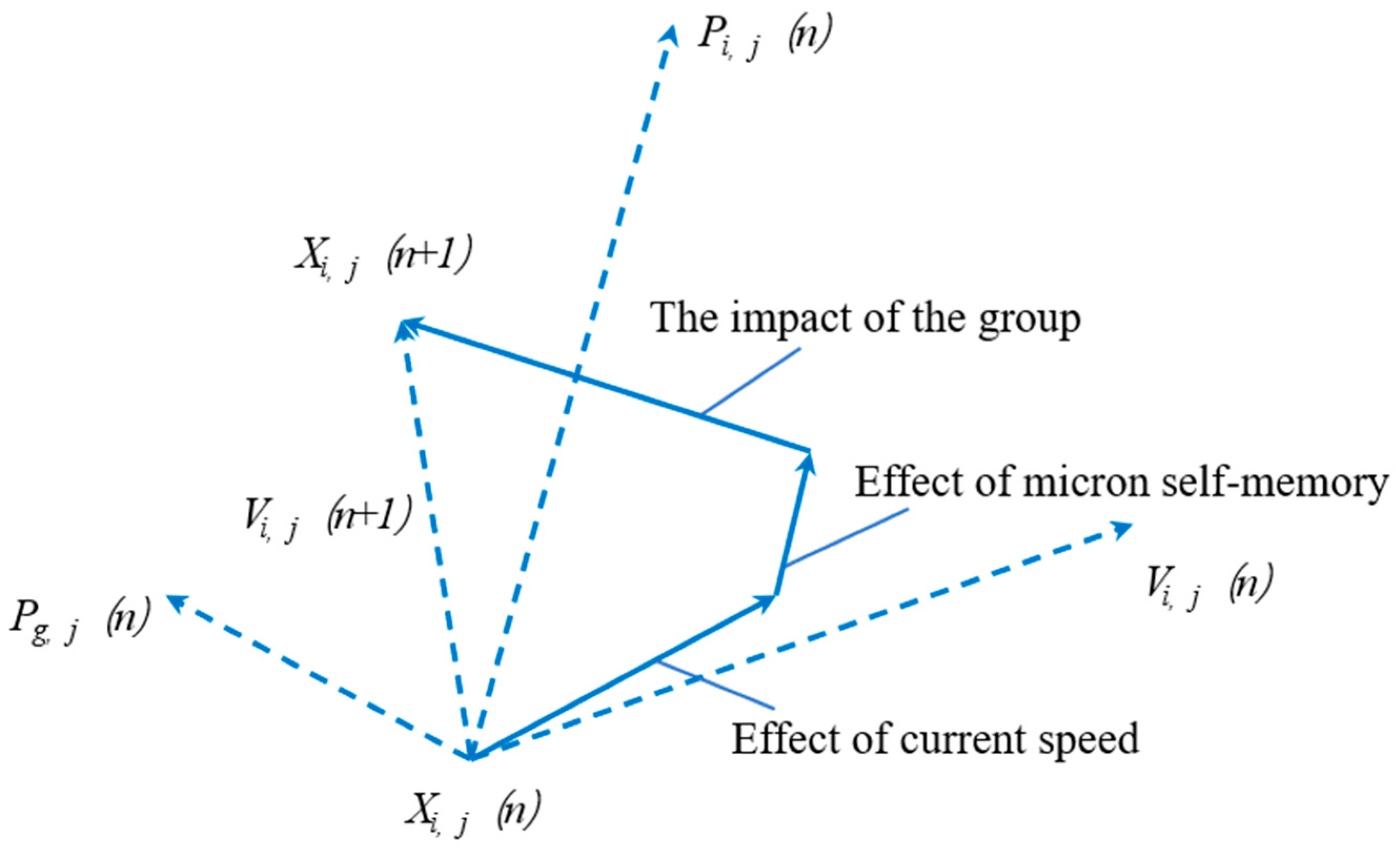
The right-hand side of Equation (6) can be divided into three parts; the first part represents the particle to maintain the travel inertia, and each particle in each iteration will inherit a part of the velocity in the previous iteration. The second part represents the influence of the particle’s own historical best position, and the particle adjusts its travel direction in the current iteration according to the optimal solution obtained in the previous iterations. The third component represents the cooperation among the particles, which adjusts the direction of travel of the particles in the current iteration according to the global optimal solution obtained by the whole particle population in the previous iterations. Three components make each particle travel purposefully to the region where the relative optimal solution may exist, and as the number of iterations increases, each particle converges to the vicinity of the optimal solution(Figure 1) [29].

Figure 1.
Particle swarm optimization schematic.
The influence of particle inertia, individual optimal solution and global optimal solution on particle travel direction is determined by changing the magnitude of inertia weight and learning factor. Generally, ε, c1, and c2 are fixed values. r1 and r2 are random numbers to provide a certain degree of perturbation in the iterations so that each particle maintains a certain degree of randomness while moving toward the global optimal solution, increasing the probability of searching for possible better solutions.
2.3. Construction of PSO Optimized LSSVM Model
- The majority of the samples obtained from the data are used as learning samples for the PSO-optimized LS-SVM model, and several examples are used as test samples. To avoid the influence of the inconsistent data dimension and to improve the training speed, the training samples are normalized to the interval [0,1].
- The initial settings of the PSO-SVM, including setting the adaptation threshold e, the particle dimension n, the population size m, the iteration number P, the learning factor c1, c2, and the inertia factor ε, randomly gives the initial solution space position Xi0 of the particle and the particle’s initial velocity Vi0.
- The test sample is predicted by the support vector machine model corresponding to each particle vector, and the prediction error of the predictive test sample is used as the individual fitness value to reflect the promotion and prediction abilities of the support vector model.where N is the number of particle samples participating in the LS-SVN training, and and are the LS-SVM training output values and expected output values of the Jth particle, respectively.
- The fitness value calculated for each particle is compared with the fitness value of the current individual optimal solution. If Si(x) < pbesti, the current particular optimal solution is replaced by the particle; that is, pbesti = Si(x), and xpbesti = xi.
- The fitness value pbesti of the current individual optimal solution of each particle is compared with the current population optimal value fitness value gbesti. If pbesti < gbesti, the particle is used to replace the original population optimal solution; that is, gbesti = pbesti, and xgbest = xi.
- After the entire group of particles is calculated, it is determined whether the termination condition is satisfied; if it is not satisfied, a new particle group is generated, and the process returns to step (3). If the termination requirement is met, the calculation ends, and the calculation result is given as an output (Figure 2).
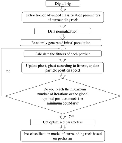 Figure 2. Flow chart of a calculation based on PSOLSSVM.
3. Case Analysis
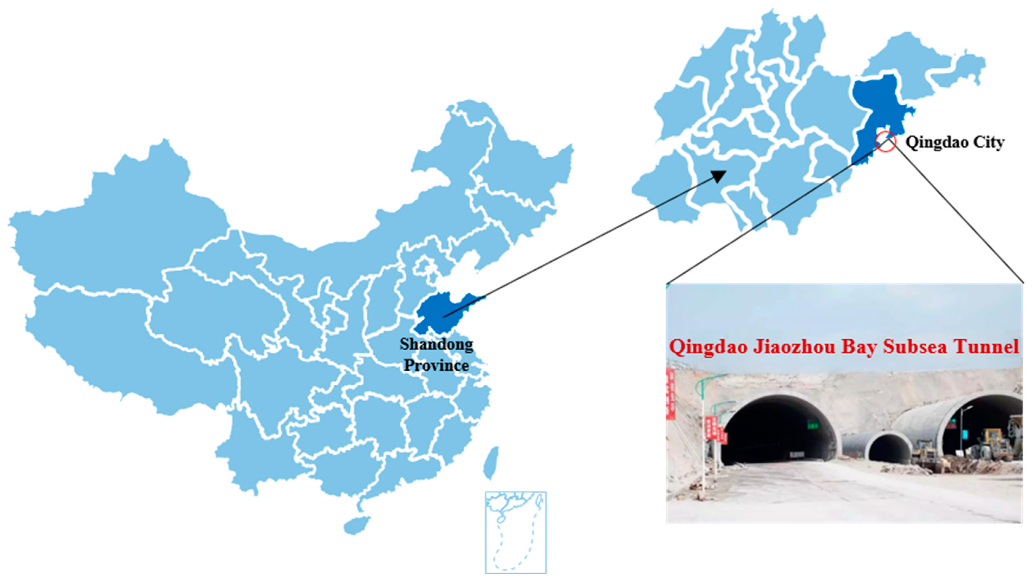
The data used in this paper are taken from Qiu et al. [30]. The Qingdao Jiaozhou Bay Undersea Tunnel is the second largest tunnel section in mainland China. The Cross-Harbour Tunnel is an important passage, which connects Qigdao’s central city and auxiliary city (Figure 3). It is connected to Xuejia Island in the south, the group island in the north, and the bay area of Jiaozhou Bay. The average depth of the sea is about 7 m, and the maximum water depth is 65 m; the maximum water depth of the bay mouth is 42 m.
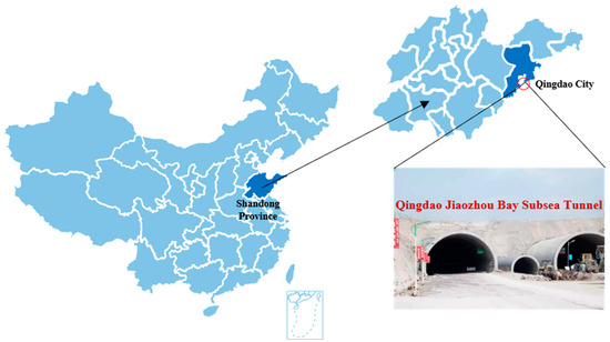
Figure 3.
Geographic location of Qingdao Jiaozhou Bay Subsea Tunnel.
General description of the geological setting:
The tunnel site area of the Jiaozhou Bay Cross Harbour Tunnel is stable, with the development of small and medium fracture structures, mainly hard rocks, with relatively intact rock masses, small permeability coefficients, more developed adverse geological effects, and generally good rock conditions. The basement rocks in the site area are mainly volcanic rocks of the Lower Cretaceous Qingshan Group and Late Yanshan Laoshan Super Unit intrusive rocks, which are hard rocks with high weathering resistance. The geological structure of the site is mainly fracture structure, in which the marine section crosses four groups and 14 fracture zones, along which there are intrusions of rock veins, with crushed rocks, fractured rocks, and vesicular rocks in the fracture zone [31].
Description of the geological setting of the subsection:
FK4+375.5: the palm wall is dominated by tuff with rhyolite. The rock is slightly weathered and relatively intact, with a predominantly blocky structure, locally with a blocky mosaic structure. The rock is relatively hard, with low permeability, and is a Class III enclosing rock.
FK4+375.5 to FK4+363.5: this section is basically the same as the current palm wall, with low strength and developed joints and fractures.
FK4+363.5~FK4+347.5: section FK4+363.5~356 has developed joints and fractures; the surrounding rock is fractured and accompanied by strong weathering soft and weak fracture filling; the surrounding rock contains water and especially around FK4+353 develops penetrating joints.
FK4+347.5~FK4+334.5: this section of the surrounding rock is broken, and the strength of the surrounding rock is poor; in the fault fracture zone, there is mud-trapping at the fault and more longitudinal fissure development.
FK4+334.5 to FK4+320.5: the section is slightly more complete than the previous section; the strength has increased, the integrity is slightly better, and the rock body is tuff.
FK4+320.5~FK4+312.5: this section still belongs to the fault fracture zone; the surrounding rock is fractured, has low strength and poor integrity, and especially at FK4+341 and FK4+345 there are more obvious fractures and it contains fractured, weak fillings.
3.1. Digital Rig
RPD-150C is the primary model employed for mine research, using a diesel engine as the power unit. The rig realizes a wide range of operations through five hydraulic cylinders, 150 m drilling and coring, and a maximum diameter of 225 mm [32,33,34,35].
Induction system: the induction system is installed on a drill or rig to obtain drilling parameters for the rig; it includes the position sensor, the rotation sensor, and the pressure sensor flow sensor.
Data conversion system: this system is used for data transmission and conversion and includes an A/D converter, which converts analog data collected by the sensor into a digital signal, and a single-chip microcomputer, which executes the programmed function program by processing the obtained digital signal and finally transmitting to the data terminal.
Data analysis system: the host computer can be placed in the test site, laboratory, or office at a remote location; it can be a computer or an external display terminal.
Digital drilling rig measurement parameters: digital drilling rig measurement parameters include shaft pressure parameters, drilling tool speed parameters, flushing water pressure parameters, and drilling speed–propulsion parameters.
3.2. Learning Samples and Test Samples
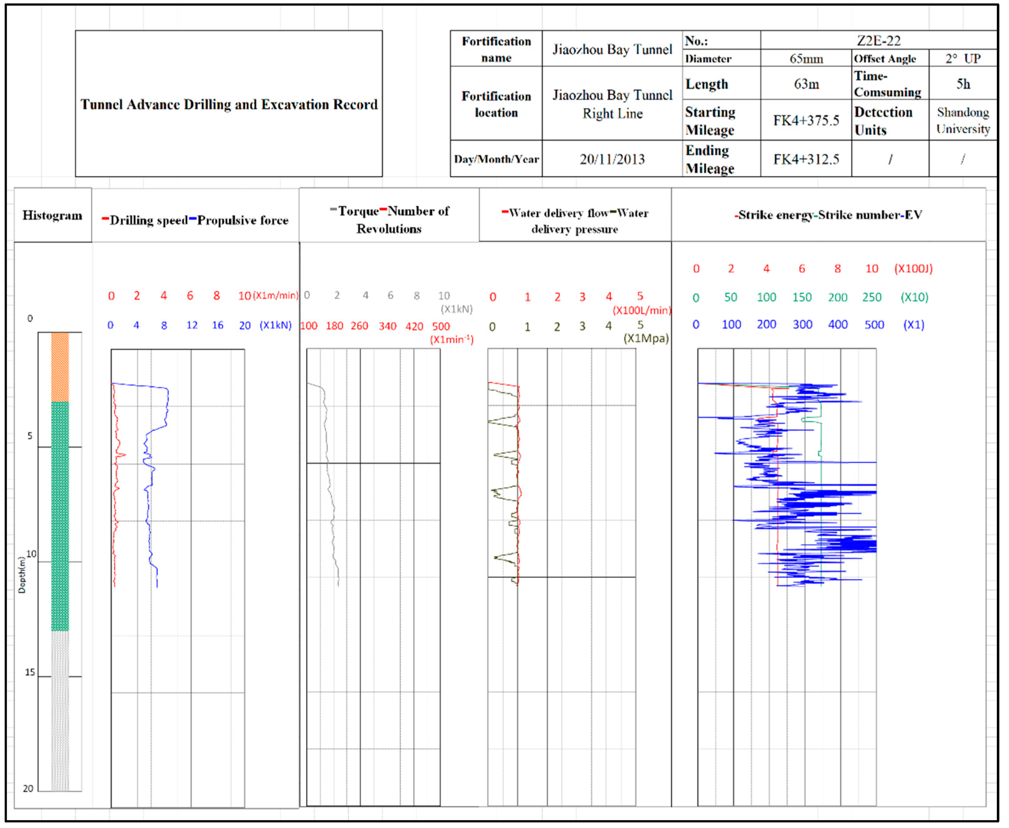
Take Qingdao Jiao Zhou Bay undersea tunnel as the engineering background, considering the valuable parameters obtained by the digital drilling rig (Figure 4). Select the index system for classifying the surrounding rock mass by selecting the speed, torque, rotation speed, propulsion force, strike energy, number of strikes, water delivery flow, and drainage flow (Table 1). For the indicator system, the numerical drilling results in the early stage of the project area and the corresponding surrounding-rock-mass classification evaluation results are selected as samples. The grade of the surrounding rock mass in the example is determined by the surrounding-rock-mass conditions that are exposed after the actual excavation. A total of 15 samples were selected (as shown in Table 2). The first 10 sets of data are used as the training set to build the prediction model, and the remaining 5 sets are used as the test set.
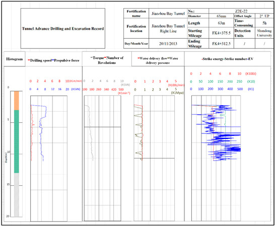
Figure 4.
Digital drilling rig parameter acquisition interface.

Table 1.
Drilling parameters.
Table 2.
Samples of drilling parameters in the Qingdao Jiao Zhou Bay Subsea Tunnel.
3.3. Model Training
The model-training process includes data normalization, parameter initialization, and iterative optimization. Data normalization uses the libsvm toolbox function scaleForSVM in Matlab to normalize the data between 0 and 1. The parameter initialization takes the particle swarm global optimization parameter c1 and the local optimization parameter c2 to 1.5, the population size m = 30, the iteration number p = 100, and the inertia factor ε0 = 0.5, and randomly generates the population and initializes the speed. Iterative optimization, the individual and the individual’s current optimal solution, the individual optimal solution, and the optimal global solution are used to continuously update the group optimal.
3.4. Dynamic Surrounding-Rock-Mass Classification
For the interest rate, the surrounding-rock-mass classification of the tunnel is generalized. Since the 1950s, the surrounding-rock-mass classification of the tunnel has been based on geological drilling, and the rock strength and integrity have been evaluated to judge the grade of the surrounding rock mass. This method is time-consuming and inaccurate. The grade of the surrounding rock mass of the tunnel is estimated, so some essential tunnels need to be detected using geological radar and seismic wave geology (TSP); then, it is necessary to generate a qualitative description of the surrounding rock mass of the tunnel. This necessitates the use of many time-consuming and labor-intensive processes, which influences the progress of the project. To promote the safe development of underground engineering, guarantee an average construction period, and reduce economic losses and environmental damage, a real-time dynamic evaluation of an artificial intelligence surrounding-rock-mass classification system is undertaken, based on cutting-edge construction methods and standardized construction management regulations. Starting from the tunnel construction process, we offer practical guidance.
At present, computer technology is the basis for the continuous development of theories and methods in the field of engineering. At the same time, it has also promoted the combination of various techniques and technologies and has produced more practical new theories. Computers have powerful data processing capabilities and fast logic operation capabilities. The empirical method in engineering often brings with it ambiguity and subjectivity. Errors often occur in construction, which increases construction volumes and economic losses. The machine learning method that uses a particle swarm optimization least squares support vector machine, and the digital drilling rig method, are applied to the classification of tunnel-surrounding rock mass. Designed as a dynamic evaluation software for the classification of tunnel-surrounding rock mass, it is a powerful method for undertaking the rapid real-time classification of surrounding rock mass in tunnels. This section uses a comprehensive method of artificial intelligence and digital drilling rigs to design a dynamic surrounding-rock-mass grade-evaluation system, based on particle swarm least squares support vector and digital rig technology, to be applied in the real-time construction of underground engineering circles. Forecasting the surrounding-rock-mass grade of the tunnel has absolute reference value. The dynamic grading interface for the surrounding rock mass is shown in Figure 5.

Figure 5.
Matlab dynamic surrounding rock grading interface.
3.5. Analysis of Results
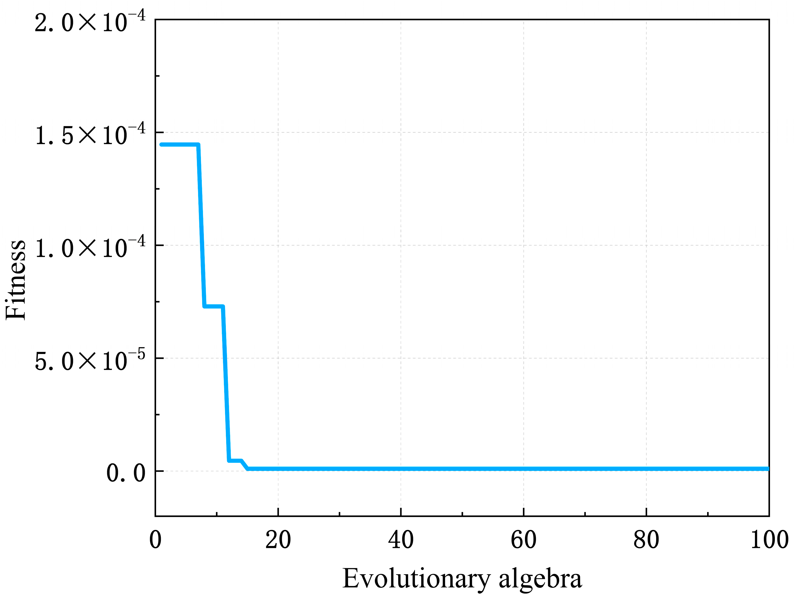
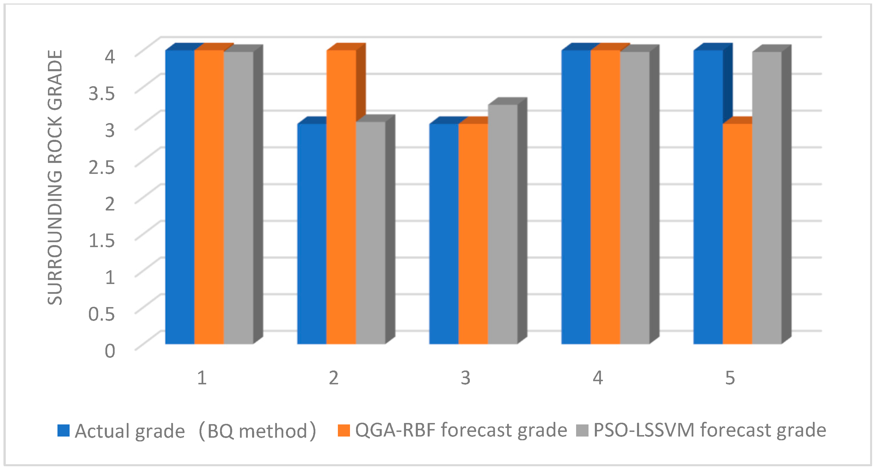
To verify the model trained by the method in engineering applications, reliability and fitness analyses in model learning (as shown in Figure 6) were undertaken. The results show that the fitness gradually decreases with the increase in the number of iterations; that is, the group tends to be optimal, and the speed is reduced most in the first 12 iterations. It is almost unchanged in the following 88 iterations. It can be seen that this method has a breakneck optimization speed and can quickly obtain the optimal global solution and analyze the test results after the model learning is completed (as shown in Figure 7), and find the classification of the method. The results are basically consistent with the results of the actual analysis (BQ classification method). It can be seen that the method is feasible in the advanced classification of surrounding-rock-mass categories, which provides a scientific basis for the construction unit to reasonably arrange the construction progress and reduce the hidden dangers of the project.
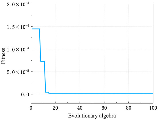
Figure 6.
Curve of fitness and evolutionary algebra (parameter c1 = 1.5 c2 = 1.5 termination algebra = 100).
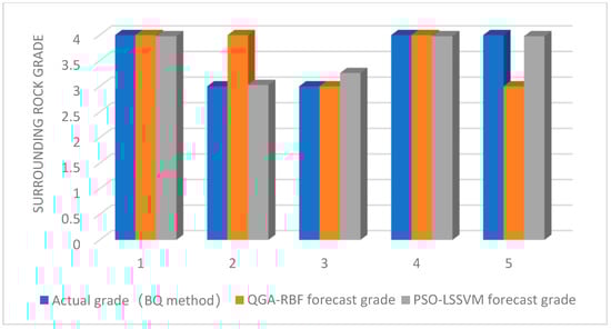
Figure 7.
Model prediction for surrounding rock grades in comparison with actual rock grades.
The method proposed in this paper is compared with traditional methods (Q method, RMR method, and BQ method).
First, in terms of the results of surrounding rock classification, the method proposed in this paper remains largely consistent with the traditional method (Table 3). Second, in terms of applicable conditions, the Q classification method is applicable in both soft and hard rock masses, and the advantages of the Q classification method are more obvious in dealing with extremely soft rock formations; the RMR method is more applicable to hard rocks affected by joints and is not suitable for use in soft rock formations; the BQ classification method is applicable to all kinds of rocks except for expansive enclosing rocks and has a wider range of use; in the above traditional methods, among the rock formations to which they are applicable, the values derived from the above traditional methods have a high degree of confidence in the rock formations to which they are applicable. The proposed method of predictive classification of surrounding rocks based on drilling parameters is applicable in both homogeneous and non-homogeneous rock masses of hard rocks but is less effective in all soft rocks. In hard rock formations, the perception of drilling parameters is more significant and its experimental results are highly accurate, while its perception of drilling parameters is weakened in soft rock formations, which can affect the experimental results. Finally, in terms of test parameter acquisition, the process of this method test (the process of deriving the results of surrounding rock classification) is simpler than the traditional method, which requires a large number of calculation parameters, and we list below the calculation equations for the various methods, as well as the calculation parameters required for this method, which require a lot of time in the field to obtain; the parameters required for the method proposed in this paper only require the drilling parameters to be derived from the digital drilling rig system, and then the rock classification can be carried out.
Table 3.
Prediction results of PSO-LSSVM compared with traditional methods.
Combining these three points we conclude that the method proposed in this paper has advantages over traditional methods.
Traditional method Q method calculation formula [36]:
Parameters to be obtained for the Q method: RQD for rock quality index, Jn for number of joint groups, Jr for joint roughness coefficient, Ja for joint alteration impact factor, Jw for joint water discount factor, and SRF for stress discount factor.
Traditional method RMR method calculation formula [37]:
Parameters to be obtained for the RMR method: A1 for rock strength, A2 for RQD values, A3 for joint spacing, A4 for discontinuous structural face characteristics, A5 for groundwater conditions, and B for the joint orientation correction factor.
Traditional method BQ method calculation formula [38]:
Parameters to be obtained for the BQ method: Rc represents the uniaxial saturation compressive strength of the rock, and Kv represents the rock integrity index.
Formula for calculating Rc: ; Is(50) represents the measured rock point load strength index.
Formula for calculating Kv: ; Vpm represents the elastic longitudinal wave velocity of the rock mass; Vpr represents the elastic longitudinal wave velocity of the rock.
4. Conclusions
In this paper, based on the problem of classifying surrounding rock mass, a method for the pre-classification of surrounding rock mass based on the particle swarm least squares support vector machine is proposed. Based on the results of the digital drilling detection, it can be concluded that this method extracts useful information, uses the particle swarm optimization least squares support vector machine parameters, establishes the prediction model, and classifies the surrounding-rock-mass categories in the front of the face. Taking as an example the data from the study by Qiu et al., “Digital Drilling Technology and Quantum Genetics-Radial Basis Function Neural Network for Advance Recognition Technology of Surrounding Rock Classes”, the algorithm was trained and tested, and the test results are basically consistent with the actual situation. In the paper, the proposed method is compared with the traditional method in terms of classification results, application scenarios, and test parameter acquisition, and it is found that the method proposed in this paper has advantages over the traditional method. As such, it can meet the necessary engineering requirements.
The accuracy of the particle swarm least squares support vector machine is improved as the number of learning samples increases. Although the training data used in this paper comprise only 10 groups, results that meet the engineering requirements can be obtained relatively quickly. The particle swarm method can quickly identify characteristics and overcome the blindness and randomness of artificial selection, and it has high precision. Under the condition of fewer samples, it can also produce results very close to the target value and has accurate positioning abilities. It is thus particularly suitable for surrounding-rock-mass classification.
This training is based on digital drilling technology, which is used to obtain the data, but it is not limited to this method. In future research, it can be used to obtain surrounding-rock-mass data based on different methods of obtaining this data (however, the data source must be accurate and reliable). In this way, the feasibility of the method can be confirmed.
Author Contributions
Conceptualization, R.Z. and Y.D.; methodology, R.Z., J.L. (Jinpei Liu) and S.S.; formal analysis, J.L. (Jie Lu) and J.L. (Jinpei Liu); investigation, W.G. and S.S.; resources, Y.D.; data curation, J.L. (Jinpei Liu); writing—original draft preparation, J.L. (Jie Lu),W.G. and S.S.; writing—review and editing, all authors; supervision, W.G. and S.S.; All authors have read and agreed to the published version of the manuscript.
Funding
This work was supported by the State Key Laboratory Open Project of China, grant number GJNY-18-73.3.
Institutional Review Board Statement
Not applicable.
Informed Consent Statement
Not applicable.
Data Availability Statement
Not applicable.
Acknowledgments
The authors would like to acknowledge the receipt of a research grant award as principal investigators from the State Key Laboratory Open Project of China under Grant No. GJNY-18-73.3. We also thank the anonymous reviewers for their constructive feedback on the initial manuscript.
Conflicts of Interest
The authors declare no conflict of interest.
References
- Wang, M.; Zhu, Y.; Li, Y.; Guo, D.; Li, W.; Wang, M. Study on stability classification of surrounding rock of coal gateway based on fuzzy clustering method. J. Min. Sci. Technol. 2018, 3, 238–245. [Google Scholar]
- Yao, J.; Wang, R.; Xia, D.H.; Deng, X.; Zhang, C. A review of the progress of tunnel envelope classification research. Highway 2021, 66, 367–372. [Google Scholar]
- Barton, N.; Lien, R.; Lunde, J. Engineering classification of rock masses for the design of tunnel support. Rock Mech. Felsmech. Mécanique Roches 1975, 12, 77. [Google Scholar] [CrossRef]
- Nicholson, G.A.; Bieniawski, Z.T. A nonlinear deformation modulus based on rock mass classification. Int. J. Min. Geol. Eng. 1990, 8, 181–202. [Google Scholar] [CrossRef]
- Sapigni, M.; Berti, M.; Bethaz, E.; Busillo, A.; Cardone, G. TBM performance estimation using rock mass classifications. Int. J. Rock Mech. Min. Sci. 2002, 39, 771–788. [Google Scholar] [CrossRef]
- Chen, L.; Chen, S.; Tu, P. Study on Mutual Relationships between Surrounding Rock Classificationsby Q Value, RMR and BQ Method for Underground Cavern. Subgrade Eng. 2017, 6, 107–112. [Google Scholar]
- Liu, X.; Gao, Y. Research on Quality Classification of Surrounding Rock Based on BP Neural Network. Water Power 2022, 48, 51–55. [Google Scholar]
- Yin, H.; Zhao, H.; Xu, L. Classification of Rock Mass in Mine Based on Improved Fuzzy Comprehensive Evaluation Method. Metal Mine 2020, 7, 53–58. [Google Scholar]
- Shao, L.; Xu, B. Research on Classification of Tunnel Surrounding Rock Based on Factor Analysis and Fisher Discriminant Analysis. J. Highw. Transp. Res. Dev. 2015, 32, 98–104+119. [Google Scholar]
- Tan, B.J.; Hardy, J.K.; Snavely, R.E. Accelerant classification by gas chromatography/mass spectrometry and multivariate pattern recognition. Anal. Chim. Acta 2000, 422, 37–46. [Google Scholar] [CrossRef]
- Meng, J.; Li, H.; Tian, W. Prediction of tunnel uplift deformation caused by foundation pit construction based on GA-BP. J. Rail Way Sci. Eng. 2019, 16, 2521–2529. [Google Scholar]
- Liu, J.; Zhang, J.; Zhu, W. Tunnel surrounding rock classification model based on bp neural network method. Beifang Jiaotong 2019, 310, 85–87. [Google Scholar]
- Guo, L.; Fu, H. Rockmass classification for meiguan tunnel based on artifical neural net. Mod. Tunn. Technol. 2010, 47, 13–17. [Google Scholar]
- Chen, P.; Yu, H.; Shi, H. Prediction model for rockburst based on weighted back analysis and standardized fuzzy comprehensive evaluation. Chin. J. Rock Mech. Eng. 2014, 33, 2154–2160. [Google Scholar]
- Song, Y.; Chen, S.; Fei, Y.; Chang, X. Fisher’s discriminant analysis method for identification and classification of expansive soil. Rock Soil Mech. 2007, 28, 499–504. [Google Scholar]
- Chen, H.; Li, X.; Liu, A.; Peng, S. Identifying of mine water inrush sources by Fisher discriminant analysis method. J. Cent. South Univ. (Sci. Technol.) 2009, 40, 1114–1120. [Google Scholar]
- Ren, Y.; Li, T.; Xiong, G.; Lin, Z. New surrounding rock classification method for high geostress tunnels and its applications. J. Eng. Geol. 2012, 20, 66–73. [Google Scholar]
- Shi, S.; Li, S.; Li, L.; Zhou, Z.; Wang, J. Advance optimized classification and application of surrounding rock based on fuzzy analytic hierarchy process and Tunnel Seismic Prediction. Autom. Constr. 2014, 37, 217–222. [Google Scholar] [CrossRef]
- Zhu, M.; Zhu, H.; Wang, X.; Cheng, P. Study on CART-based ensemble learning algorithms for predicting TBM tunneling parameters and classing surrounding rockmasses. Chin. J. Rock Mech. Eng. 2020, 39, 1860–1871. [Google Scholar]
- Li, J.; Zheng, Y.; Jing, L.; Chen, S.; Jian, P.; Yu, T.; Zhao, Y. TBM tunneling parameters prediction method based on clustering classification of rock mass. Chin. J. Rock Mech. Eng. 2020, 39, 3326–3337. [Google Scholar]
- Li, H. Prediction and Identification Method of Tunnel Boring Machine Surrounding Rock Grade Based on Tunneling Parameters Inversion. Tunn. Constr. 2022, 42, 75–82. [Google Scholar]
- Qiu, D.; Li, S.; Zhang, L.; Xue, Y.; Su, M. Prediction of surrounding rock classification in advance based on TSP203 system and GA-SVM. Chin. J. Rock Mech. Eng. 2010, 29, 3221–3226. [Google Scholar]
- Xue, Y.; Li, S.; Zhang, Q. Application of TSP203 advanced prediction to tunnel in karst areas. Chin. Undergr. Space Eng. 2007, 3, 1187–1191. [Google Scholar]
- Huang, X.; Shi, L.; Suykens, J.A.K. Asymmetric least squares support vector machine classifiers. Comput. Stat. Data Anal. 2014, 70, 395–405. [Google Scholar] [CrossRef]
- Van Gestel, T.; Suykens, J.A.K.; De Brabanter, J.; De Moor, B.; Vandewalle, J. Least squares Support Vector Machine regression for discriminant analysis. In Proceedings of the IJCNN’01: International Joint Conference on Neural Networks, Washington, DC, USA, 15–19 July 2001; Volume 1–4, pp. 2445–2450. [Google Scholar]
- Van Gestel, T.; Suykens, J.A.K.; Lanckriet, G.; Lambrechts, A.; De Moor, B.; Vandewalle, J. Bayesian framework for least-squares support vector machine classifiers, Gaussian processes, and kernel Fisher discriminant analysis. Neural Comput. 2002, 14, 1115–1147. [Google Scholar] [CrossRef] [PubMed]
- Suykens, J.A.K.; Van Gestel, T.; Vandewalle, J.; De Moor, B. A support vector machine formulation to PCA analysis and its kernel version. IEEE Trans. Neural Netw. 2003, 14, 447–450. [Google Scholar] [CrossRef] [PubMed]
- Long, W.; Liang, X.M.; Long, Z.Q. Parameters selection for LSSVM based on modified ant colony optimization in short-term load forecasting. J. Cent. South Univ. (Sci. Technol.) 2011, 42, 3408–3414. [Google Scholar]
- Hou, X.; Sun, Y.; Wu, J. Magnetic field modelling of ship using magnetic dipole array based on pso algorithm. Ship Sci. Technol. 2022, 44, 159–164. [Google Scholar]
- Qiu, D.; Li, S.; Xue, Y. Advanced prediction of surrounding rock classification based on digital drilling technology and QGA-RBF neural network. Rock Soil Mech. 2014, 35, 2013–2018. [Google Scholar]
- Tian, H. Refinement Identification Method of Digital Drilling for Tunnel Geological; Shandong University: Jinan, China, 2015. [Google Scholar]
- Tian, H.; Li, S.; Xue, Y.; Qiu, D.; Su, M. Identification of interface of tuff stratum and classfication of surrounding rock of tunnel using drilling energy theory. Rock Soil Mech. 2012, 33, 2457–2464. [Google Scholar]
- Tan, Z.; Cai, M.; Yue, Z.; Tan, G.; Li, Z. Interface identification of intricate weathered granite ground investigation in hong kong using drilling parameters. Chin. J. Rock Mech. Eng. 2006, 25, 2939–2945. [Google Scholar]
- Zou, X.; Chao, A.; Ye, T.; Nan, W.; Zhang, H.; Yu, T.Y. An experimental study on the concrete hydration process using Fabry–Perot fiber optic temperature sensors. Measurement 2012, 45, 1077–1082. [Google Scholar] [CrossRef]
- Chao, A. Investigation of Portland Cement Concrete Hydration Behavior at Its Early Age Using embedded Fiber Optic Temperature Sensors; University of Massachusetts Lowell: Lowell, MA, USA, 2011. [Google Scholar]
- Barton, N.; Lien, R.; Lunde, J. Engineering classification of rock masses for the design of tunnel support. Rock Mech. 1974, 6, 189–236. [Google Scholar] [CrossRef]
- Bieniawski, Z. Engineering Rock Mass Classifications; The Wiley-Interscience Publication: New York, NY, USA, 1989. [Google Scholar]
- GB50218-94; Standard for Engineering Classification of Rock Masses. Ministry of Water Resources of the People’s Republic of China: Beijing, China, 1995.


Disclaimer/Publisher’s Note: The statements, opinions and data contained in all publications are solely those of the individual author(s) and contributor(s) and not of MDPI and/or the editor(s). MDPI and/or the editor(s) disclaim responsibility for any injury to people or property resulting from any ideas, methods, instructions or products referred to in the content. |
© 2023 by the authors. Licensee MDPI, Basel, Switzerland. This article is an open access article distributed under the terms and conditions of the Creative Commons Attribution (CC BY) license (https://creativecommons.org/licenses/by/4.0/).