Abstract
In the field of adversarial attacks, the generative adversarial network (GAN) has shown better performance. There have been few studies applying it to malware sample supplementation, due to the complexity of handling discrete data. More importantly, unbalanced malware family samples interfere with the analytical power of malware detection models and mislead malware classification. To address the problem of the impact of malware family imbalance on accuracy, a selection feature conditional Wasserstein generative adversarial network (SFCWGAN) and bidirectional temporal convolutional network (BiTCN) are proposed. First, we extract the features of malware Opcode and API sequences and use Word2Vec to represent features, emphasizing the semantic logic between API tuning and Opcode calling sequences. Second, the Spearman correlation coefficient and the whale optimization algorithm extreme gradient boosting (WOA-XGBoost) algorithm are combined to select features, filter out invalid features, and simplify structure. Finally, we propose a GAN-based sequence feature generation algorithm. Samples were generated using the conditional Wasserstein generative adversarial network (CWGAN) on the imbalanced malware family dataset, added to the trainset to supplement the samples, and trained on BiTCN. In comparison, in tests on the Kaggle and DataCon datasets, the model achieved detection accuracies of 99.56% and 96.93%, respectively, which were 0.18% and 2.98% higher than the models of other methods.
1. Introduction
In recent years, deep learning has been widely used for adversarial attacks. Despite the high accuracy of existing malware detection systems, the accuracy of detection for various samples remains low, especially for a few malware attacks, leading to the misclassification of such and failure to meet the requirements of accuracy. More importantly, in the malware space, it is becoming increasingly important to address malware family sample imbalances and improve detection accuracy.
The imbalance problem is often used to improve model training by increasing the number of samples in a dataset, and much research has been conducted based on this approach. Although many methods are being evaluated with inadequate or unbalanced datasets, the actual performance is still open to improved discussion. For example, some studies have been validated by using a restricted number of sample sizes [1]. Although limited generalization performance was demonstrated, this does not indicate effectiveness against newly generated malware. The reason for this is that the training set contains samples of existing malware families but has difficulty detecting newly new variants of malware.
In intelligent malware detection, relevant features (e.g., task, intent, application programming interface calls, system calls, and byte features) are extracted in advance and used in the training of malware detectors with better results [2]. The effectiveness of machine learning models depends on the assumption that training and test data follow the same distribution, an assumption that is likely to be corrupted by attackers, compromising the security of the models. An attacker can force a classification model to output incorrect predictions by applying a small perturbation on the input samples in what is called an adversarial sample attack. In the area of malware, attackers exploit the deficiencies of the model to generate malware samples for the purpose of bypassing malware detectors [3,4].
To avoid this problem, the study considered time series features [5,6]. Because these methods use a balanced dataset to evaluated malware models, many previous studies have therefore not considered class imbalance and can be unstable on unbalanced datasets. For this reason, this paper uses two unbalanced datasets and compares the results with other models. This paper proposes a new attack framework selection feature, the conditional Wallenstein generative adversarial network (SFCWGAN), which uses the generative adversarial network (GAN) to generate attack loads. Feature selection can filter out redundant features, simplify the data structure, and improve the accuracy of malware detection. This paper therefore focuses on a malware classifier based on the temporal convolutional network (TCN) variant detection model. To generate continuous adversarial instances from the sequence of API and Opcode calls, perturbations are considered for API and Opcode calls and inserted into the original sequence. The original features use WordVec to represent the API and Opcode call sequences, and interfering obfuscated API and Opcode calls are inserted in the sequences. The samples are extended using the conditional Wallenstein generative adversarial network (CWGAN) to balance the sample distribution and combined with the bidirectional temporal convolutional network (BiTCN) to mine deep temporal features from the sequence features, and thus improve the detection accuracy.
The following contributions are made in this paper.
- SFCWGAN-BiTCN, a malware detection approach based on SFCWGAN and BiTCN, is proposed to mitigate the interference of malware family sample imbalance on detection accuracy.
- A new word-embedding method is designed in conjunction with the Word2Vec algorithm to obtain API and Opcode call sequences in the order of their virtual addresses and map them into a vector space, exploiting the sequential semantics of the API and Opcode call contexts.
- Feature selection and merging using whale optimization algorithm extreme gradient boosting (WOA-XGBoost) and Spearman correlation coefficients reduces redundant features, simplifies the Word2Vec feature, and improves detection accuracy and efficiency.
- The use of CWGAN to generate imbalanced malware family samples to supplement the dataset enhances model training, reduces the effect of malware family sample imbalance on detection, and improves detection accuracy.
- The BiTCN extracts time-varying features in malware sequences for deep feature mining of time series by improving the TCN model, in order to fully exploit temporal features.
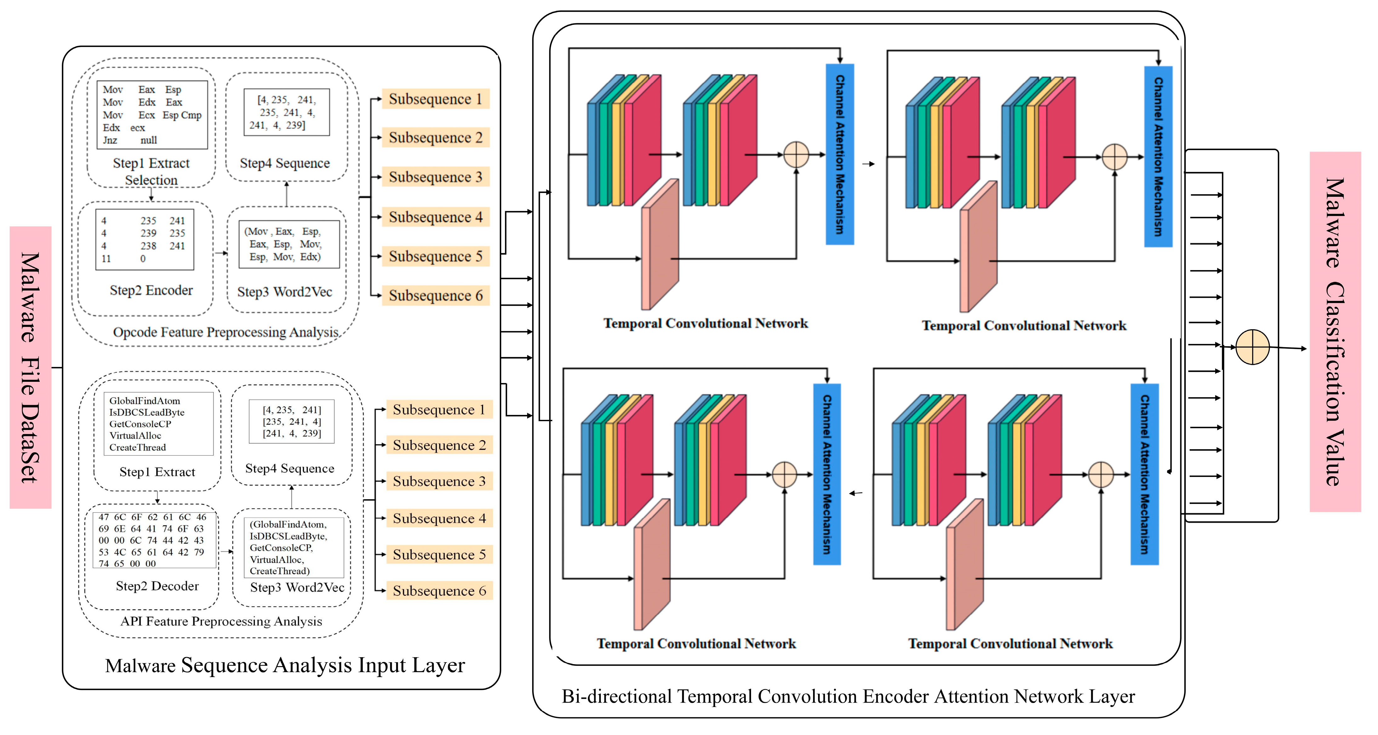
- The malware detection structure is shown in Figure 1.
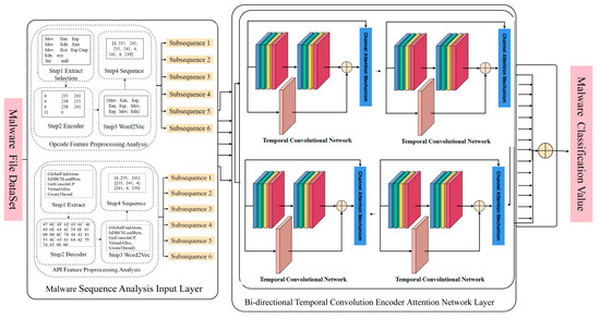 Figure 1. SFCWGAN-BiTCN-based malware detection framework.
2. Related Work
2.1. Unbalanced Datasets
In the classification and learning of unbalanced data, the problem of classifying unbalanced multi-view data has been a hot research topic in the field of network neuroscience. An intuitive approach is to obtain a balanced distribution of data by sampling methods, which include oversampling, under sampling, or synthetic sampling. An advanced synthetic sampling method called SMOTE [7] adds artificial examples created by interpolating neighboring data points. Following this work, security-level SMOTE [8] proposed a weighted generation process to make the data synthesis process more robust. Graa and Rekik [9] proposed a multi-view learning-based data multiplier (MV-LEAP) that can classify unbalanced multi-view representations. Fu et al. [10] proposed an algorithm called ssHD to achieve stable sparse feature selection and apply it to complex classes of imbalanced data. Cui [11] first proposed a new approach to improve malware detection using a new deep learning model. In this approach, the bat algorithm addresses the problem of class imbalance between different malware families, which is a frequent problem in data-based cybersecurity-related research. The BAT algorithm equalizes the data, and then a model of CNN is used to detect malware variants.
2.2. Generative Adversarial Networks (GANs)
In the process of adversarial training of malware detectors, the generation of adversarial samples is an important aspect. It is an important issue in the field of malware to generate realistic malware adversarial samples with low attack cost and high attack success rate by exploiting the knowledge of adversarial samples. The GAN proposed by Goodfellow et al. [12] has an advantage in sample generation. The GAN consists of a generator and a discriminator, and through the game between the generator and the discriminator, the generator will learn the underlying patterns of the data and generate new data. Kim et al. [13] used the GAN to generate samples of malware based on grayscale images. Later, Kim et al. [14] used a deep convolutional GAN model to generate malware samples based on the literature [13] and simulated the generation of zero-day malware based on image structural similarity. The literature [15] uses an auxiliary classification generation adversarial network to generate grayscale images of malware but does not consider the quality of malware generated by the generator. Due to the structural interdependencies between adjacent bytes of the malware, any changes to the malware file may corrupt the executable and affect the function of the malware [16]. Unlike adversarial images, malware adversarial samples are not executable in the real world, even if they successfully spoof the detection model.
On the problem of malware excitability, Hu et al. [17] proposed a GAN-based malware generation algorithm that implements a black-box attack on malware detectors by introducing an alternative detector and achieves malware countermeasure sample generation by adding a scrambled application programming interface (API) to the import table. However, malware generation based on the original GAN model is prone to problems, such as gradient disappearance and training instability. The limitation of the algorithm is that the perturbation of the sequence is not continuous, and the study does not consider the cost of the attack in the adversarial generation process. Tang Chuan et al. [18] proposed an adversarial sample generation algorithm based on a minimum modification cost, using a deep convolutional GAN model to generate benign perturbations and by modifying the decompiled file and repackaging the Android application package (APK) to generate an executable malware adversarial sample, which successfully bypassed the detection of the target detector. However, this method only takes into account the modification cost of the malware features and not the number of queries from the malware detectors during the generation of the adversarial samples. Due to the multiple repeated queries of the detector, which are easily detected by security personnel, attackers need to consider the target detector query efficiency when attacking the detector.
Rosenberg et al. [19] generated an adversarial sample by repeatedly modifying the API call sequence and non-sequence features of the malware. For the purpose of preserving sequence semantic information, only some invalid API calls were inserted into the original sequence. Jha et al. [20] proposed a Word2Vec embedding model based on malware identification, combining feature vectors obtained from RNNs and skip grams but vulnerable to obfuscation techniques. Gibert et al. [21] feature byte sequences, API function calls and Opcodes using a LeNet5 structure based on the Word2Vec multichannel feature matrix but with different colors for different features, which ignores the correlation between features. However, classification techniques rely on APIs, and operand sequence patterns can be interfered with by inserting irrelevant information. Malware authors can therefore easily mislead static and dynamic analyses that rely on computing statistical properties or identifying the malware sequence patterns of API calls.
In summary, most of the above deep learning-based approaches are targeted at sequence features for classification and detection. For the problem of class imbalance among malware families, the traditional methods show limitations, and the impact of interference obfuscation techniques on existing malware classification models is not considered.
3. SFCWGAN and BiTCN
The scheme proposed in this paper extends SeqGAN [22] using a sequence-based generator to generate sequence samples of malware. A malware detection method based on SFCWGAN and BiTCN is designed. WOA-XGBoost is used to rank the importance of the features, and using coefficient-based Spearman correlation analysis. The feature structure is simplified by filtering out features with strong correlation and retaining the important ones. The generated samples and the original samples are trained using BiTCN and validated by comparing the samples captured in the existing network.
3.1. CWGAN
The GAN is inspired by game theory, where it is used for modelling complex distributions of real-world data. It consists of a generator (G) and a discriminator (D) [23]. The generator captures the underlying distribution of real data samples and generates new data samples. The discriminator is a binary classifier that determines whether the input samples are real or generated [24]. The optimization process is a min-max game problem whose goal is to keep a balanced sample distribution. The objective function for the GAN is:
where represents the distribution of the real samples, maps the noise to the space, is the samples, and is the probability of the real data. To distinguish data, is large and is as small as possible. CGAN is based on a GAN in which malware families are merged with the original samples as inputs, with the loss function:
where is noise, is malware family.
The traditional GAN and its variants are used to generate samples and reduce the impact of sample imbalance in malware families. However, this can lead to vanishing gradient problems.
To deal to these problems, we introduced the Wasserstein distance in CGAN to implement CWGAN, and the workflow is shown in Figure 2.
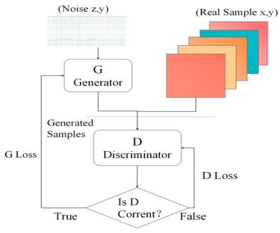
Figure 2.
CWGAN structure.
We use discriminators to determine the true samples from the generated samples. If they are indistinguishable, the G is saved and the D is trained, and if they are distinguishable, the D is saved and the G is trained. These steps are repeated until the loss function of the discriminator stabilizes at 0.05, at which point the attack samples are generated and added to the dataset.
Based on this approach, the model can generate samples to complement the dataset while effectively avoiding gradient disappearance due to the discriminator’s inability. The objective function is:
The parameter, , is the formula for calculating to , and is the middle position between and .
3.2. BiTCN
To avoid the gradient disappearance and explosion problems of CNN, enhance the ability to extract temporal features, and mine bidirectional information to further improve the classification accuracy, the classification method of BiTCN is introduced to enhance the generalization ability and classification accuracy of the malware variants. On the one hand, the API calls reflect the malware behavior of the malware and can avoid the effects of the obfuscation techniques. Assembly sequences reflect the control behavior over the system kernel and can compensate for the inability to distinguish polymorphic APIs. On the other hand, the convolutional network in a TCN [25,26] has the property of parallelizable computation, which can effectively solve the problem of excessive time consumption and has been proven to be superior to traditional RNN and its variants in several fields. However, single-item TCNs cannot encode information from back to front, resulting in the inability to capture the association between current and subsequent feature items. The introduction of BiTCN into malware classification has improved both its anti-confusion capability and accuracy.
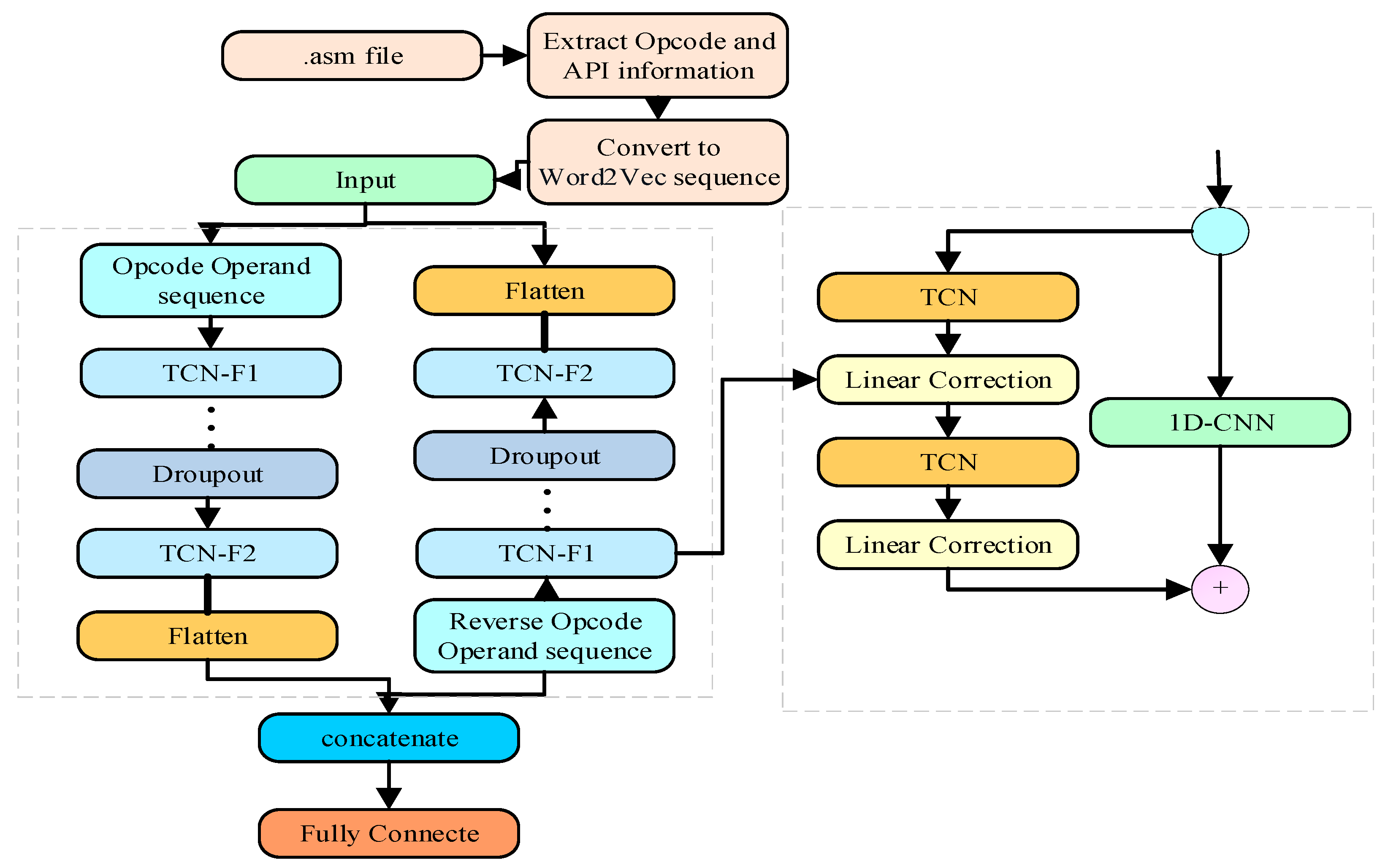
The approach in this paper extracts feature sequence features by virtual address, combined with the Word2Vec algorithm for feature representation, using a TCN network end-to-end module fused with the ability to blend the advantages of both features, describing domain-specific features and deep learning to automatically extract a set of descriptive features without relying on domain knowledge. This reduces the interference of adversarial techniques and improves accuracy and robustness. The framework of the BiTCN-CNN malware classification approach is shown in Figure 3.
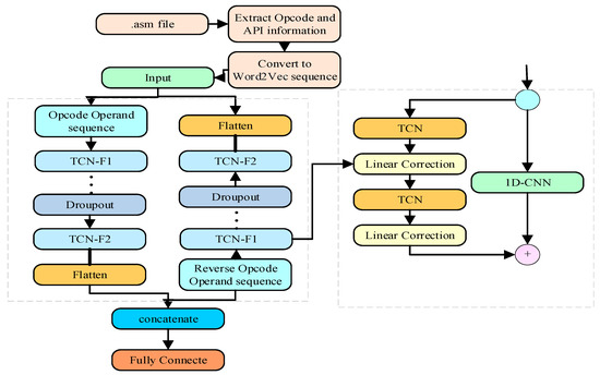
Figure 3.
Multi-feature fusion BiTCN malware classification method.
The main classification process of BiTCN consists of bidirectional feature extraction and classification. The sequence features are first processed into the sequence using Word2Vec, as described in the previous section. The features are fed into the forward and reverse TCN modules, which consist of three residual blocks with a global Dropout layer between them, with the aim of efficiently extracting sequence and global multi-level features through the three residual blocks with increasing convolution coefficients. Each residual block structure is performed sequentially and connected after two temporal convolution and Relu activation function operations. The BiTCN processing is shown in detail as follows.
After inputting the pre-processed features into the convolution, in order to solve the correlation problem of the calling sequence, the Word2Vec method is used to let the sequence repeat and enhance the feature correlation, which is conducive to extracting the temporal features of the distance unit more fully and improving the recognition performance.
The depth model contains many parameters that may lead to overfitting problems, which is not conducive to improving the generalization ability of the model. To alleviate the overfitting problem, Dropout is used as a mitigation model between residual blocks, which makes a certain percentage of nodes randomly deactivate during the training process to alleviate the effect of redundant features on the model, thus improving the generalization ability.
Finally, the fused features are fed into the fully connected layer and Softmax regression is introduced as a classifier, with the output nodes corresponding to the probabilities of the sample categories respectively. This is processed as follows:
where is the output of the classification layer, is the output of the fusion layer, indicates the trainable parameters of the classification layer, indicates the category to which it belongs, and N is the total number of categories.
3.3. Feature Pre-Processing
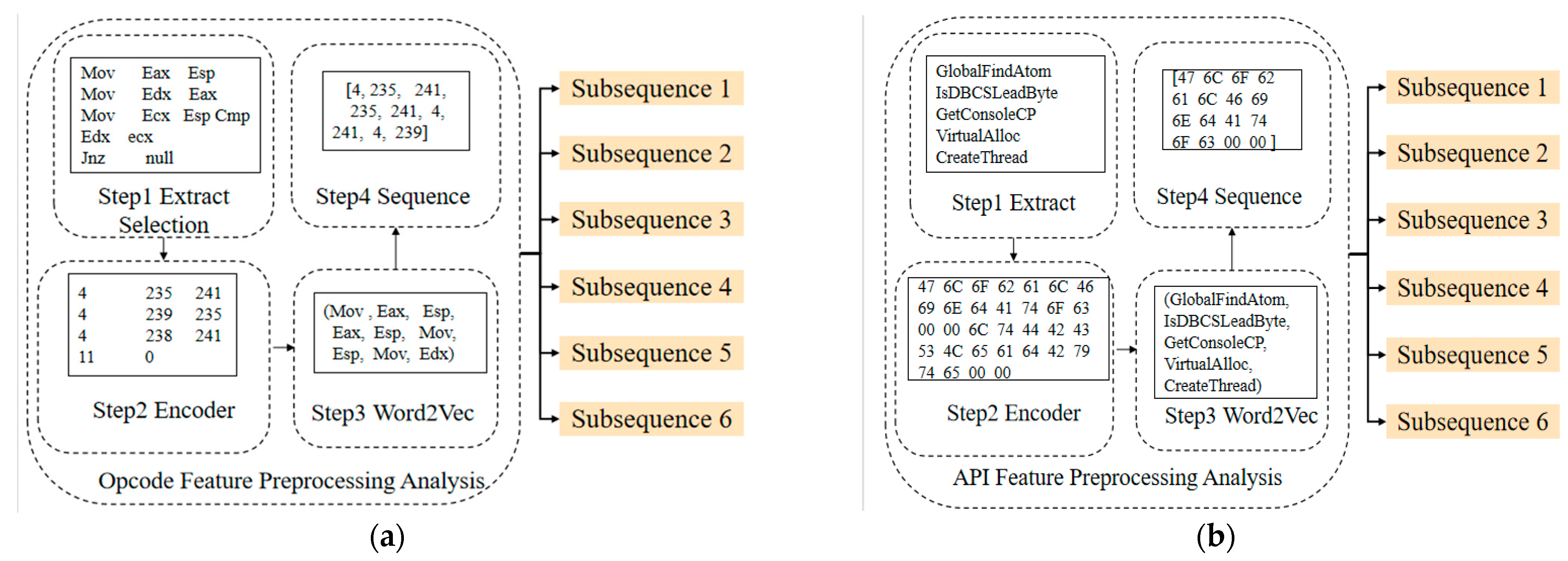
The feature pre-processing is carried out to extract and encode the API and opcode of the Kaggle and DataCon datasets. The API and Opcode information will be extracted from the .asm disassembly file of the Kaggle dataset, and the DataCon dataset is disassembled into the .asm file using IDA Pro tool, from which API and Opcode information will be obtained. Based on the virtual addresses, the whole sequence of API calls and Opcodes are generated and populated with the Opcode and API vector matrices corresponding to the virtual addresses. Finally, the sequence features are generated by encoding the vector matrix using Word2Vec. The features are pre-processed as Figure 4.
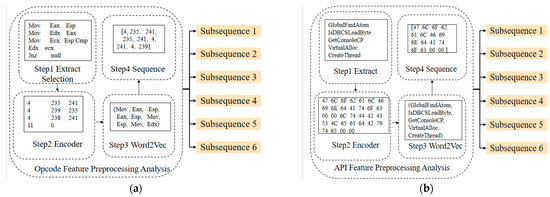
Figure 4.
Feature pre-processing. They should be listed as: (a) Opcode feature preprocessing; (b) Api feature pre-processing.
Encoding is used to convert serial features in the Kaggle and DataCon datasets to numeric types. The function used to determine whether there are null values in the dataset and normalize the data:
where and are the minimum and maximum values of the dimensions.
3.4. Feature Pre-Processing
Feature selection is a method of selecting relevant features of a dataset by obtaining a subset from the original set of features based on specific criteria.
3.4.1. WOA-XGBoost
Chen proposed [27] extreme gradient boosting (XGBoost), a modeling framework based on the idea of gradient-propelled decision trees. The core idea of XGBoost is to fit the residuals of previous predictions and keep optimizing them in successive iterations. While the traditional gradient boosting decision tree (GBDT) algorithm includes only first-order derivatives, the XGBoost algorithm [28] uses the second-order tai of the loss function and a typical term to prevent overfitting. The importance of the features is ranked using this method.
In the feature selection stage, the features are ranked for importance using the whale optimization algorithm extreme gradient boosting (WOA-XGBoost), and the relevance of the features is analyzed using Spearman’s correlation coefficient. Unlike traditional GBDT algorithms, the WOA-XGBoost algorithm expands the loss function by using second-order Taylor with a regularization term to improve the speed of model training and prevent overfitting:
where is the loss function the difference between the value of predicted and the true and is prevented overfitting; where is the number, represents the leaf weights, reduces the nodes, is the penalty factor, is the regularization, and is factor.
XGBoost requires several iterations, the objective function for the tth iteration is:
using to reduce overfitting.
The reasonableness of structure can be assessed in the light of the structural losses, that
where and are the first- and second- order derivatives of the loss function on the predicted values after iterating , and is the index of the leaf node . A smaller structural loss indicates a better decision tree structure. If the tree splits at the node , the structural gain of the leaf node is:
where is the factor, used to reduce the complexity of the structure. The splitting gain is used to control the number of the splitting nodes.
WOA [29] is a population-based algorithm. WOA-XGBoost [30] humpback whales are able to use certain abilities to determine the location of their prey when encircling them by echoing them. The position update formula is:
where denotes the current position, denotes the vector of the iteration, the best solution is denoted as , and is the vector dimension. and in [0, 1]. in [0, 2]. It can be measured with this function:
Humpback whales use contraction mechanisms and spirals to update their position when using bubble nets to catch their prey. As the median value of the formula decreases, the prey is surrounded.
Humpback whales search for prey by contracting, with the new position being between the current position and the optimal position (). The following is a model of the spiral update position:
The shape is controlled by , and the random number is obtained in the interval [−1, 1]. Mirjalili et al. [31] proposed a 50% probability of updating the existing position of the humpback whale by updating the spiral position.
When the coefficient vector , the study of humpback whale prey predation is modelled as follows:
where represents the location vector of randomly selected individual whales from the current population.
3.4.2. Spearman’s Correlation Coefficient
Spearman’s correlation coefficient is used to mine the correlation between features. Spearman is a measure of the strength of the relationship between two variables [32] and in the range (0, 1). Spearman’s correlation coefficient is calculated as follows:
The vectors includes and . The value of A, 1 indicates a strong association and should be removed from the others. 0 indicates no association, and the features should be kept.
The features are ranked according to their importance and analyzed using Spearman’s correlation coefficient. The features are combined to filter out irrelevant features, retain important features, and input to the GAN for malware family sample generation.
3.5. Sample Generation
During the generation of malware family samples, CWGAN is trained using the feature selection and noise samples in Algorithm 1. The process of CWGAN is as follows:
| Algorithm 1: Minority class sample generation based on CWGANs |
| , where is noise data and is class label |
| 1. the generator and discriminator generator parameters , discriminator parameters , the gradient penalty , Adam learning rate |
| 2. While does not approach 0.05/*CWGAN training */ |
| 3. for do/*optimize discriminator */ |
| 4. Sampling form |
| 5. Sampling form |
| 6. /*calc gradient */ |
| 7. /*updata hyperparameters */ |
| 8. end |
| 9. form sample /*optimize discriminator */ |
| 10 /*calc gradient */ |
| 11 /*updata hyperparameters */ |
| end |
| return/*generate samples */ |
3.6. Feature Extraction and Training
During the feature extraction phase, the BiTCN layer learns temporal features in the dataset, Nadam optimization is used as an optimizer, the Dropout layer mitigates overfitting, and the Softmax classifier is used for malware classification.
To avoid the overfitting problem in the training process, we used two methods. First, the number of samples of some families is too small, leading to overfitting of training, which requires balancing the dataset by generating malicious samples with the GAN. Second, as the model is too large, dropout is used to cull the BiTCN model to avoid overfitting. The whole dropout process is equivalent to averaging the neural network. When the network is overfitted, some of the “reverse” fits cancel each other out to reduce the overall overfitting.
4. Experiments and Analysis of Results
4.1. Datasets
4.1.1. Kaggle
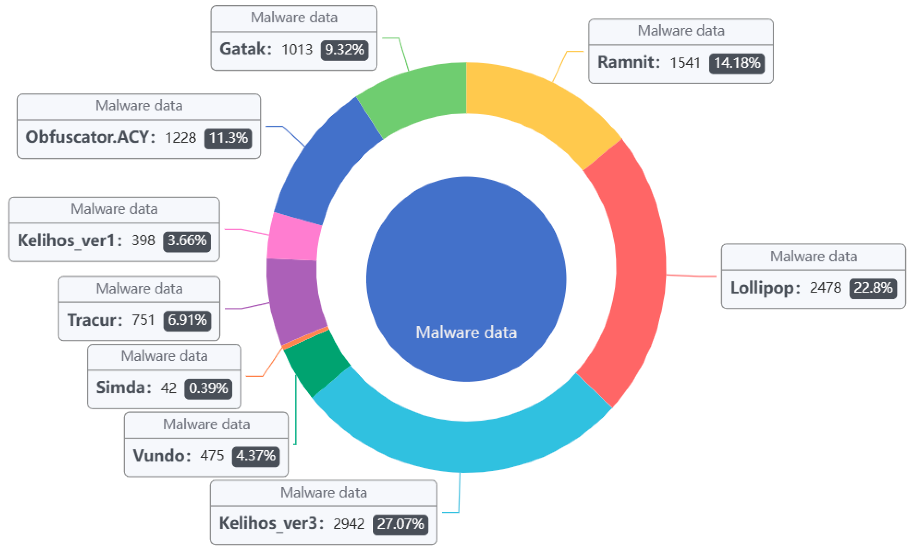
The Kaggle [33] malware data set utilized the samples (see Figure 5 and Table 1). The malware families in the dataset provided by Microsoft were divided into nine categories, a total of 10,868 malware samples. Each sample file has two formats: .asm and .bytes. Each malware file has an identifier (a 20-character hash that uniquely identifies the file), and a class label (an integer that indicates one of the nine family names to which the malware belongs). In addition to this, the dataset not only includes the list of raw data, but also contains logs of various raw data information extracted from the binary files, (e.g., function calls, API, and parameters).

Figure 5.
Kaggle dataset sample distribution.

Table 1.
Quantity Distribution of Sample Kaggle Dataset.
4.1.2. DataCon
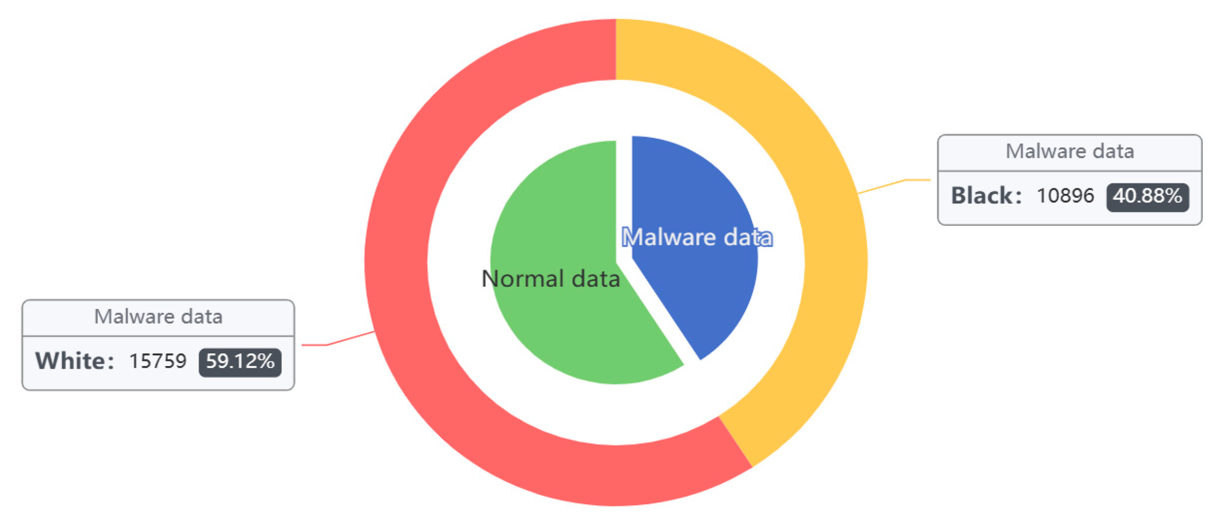
The DataCon [34] data samples are all real data captured by the existing network, including a significant number of encryption, obfuscation, and real malware samples. These include 7896 mining samples and 15,759 malware samples of other families, for a total of 23,655. Analyzing the statistics shows the dataset contains a variety of samples with compressed or encrypted shells of UPX, PEPack, ASPack, PECompact, Themida, VMP, and Mpress shells with encrypted shells and disguised shells, etc. In this paper, the DataCon dataset was utilized as a comparison experiment to verify the effectiveness of the method in this paper when applied to real datasets (see Figure 6 and Table 2).
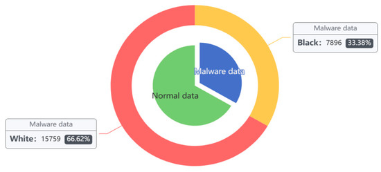
Figure 6.
DataCon dataset sample distribution.
Table 2.
Quantity Distribution of Sample DataCon Dataset.
4.2. Experimental Assessment Criteria
The proposed model was evaluated on the Kaggle and the DataCon datasets captured on the present network. The evaluation Indicators were used to determine the classification effectiveness of the model. The experiment selected common evaluation criteria in the field of malware classification detection—Accuracy, Precision, Recall, and f1-score—to evaluate the classification of the network. These criteria are calculated as follows:
4.3. Experimental Results and Analysis
Malware detection methods based on SFCWGAN and BiTCN are evaluated based on the following experiments:
- Accuracy analysis experiments
- Noise analysis experiments
- Comparison of difference sample balance algorithms
- Ablation experiments
- Comparison of difference classification algorithms
- Comparison of existing methods
4.3.1. Accuracy Analysis Experiments
In this paper, we use SFCWGAN- and BiTCN-based malware detection methods to verify the accuracy of the model in malware detection. XGBoost is used in combination with several optimization algorithms to analyze the importance of features.
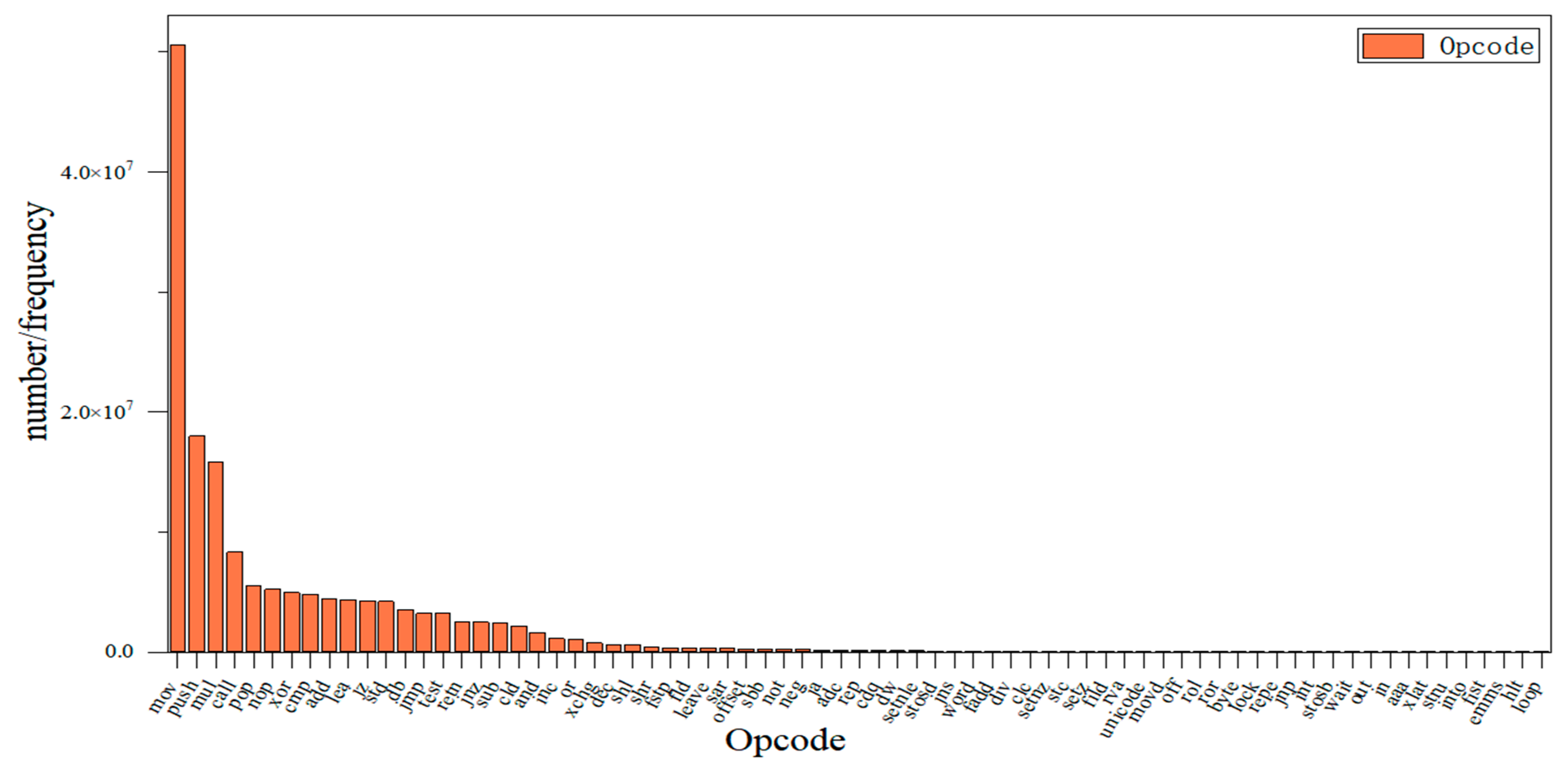
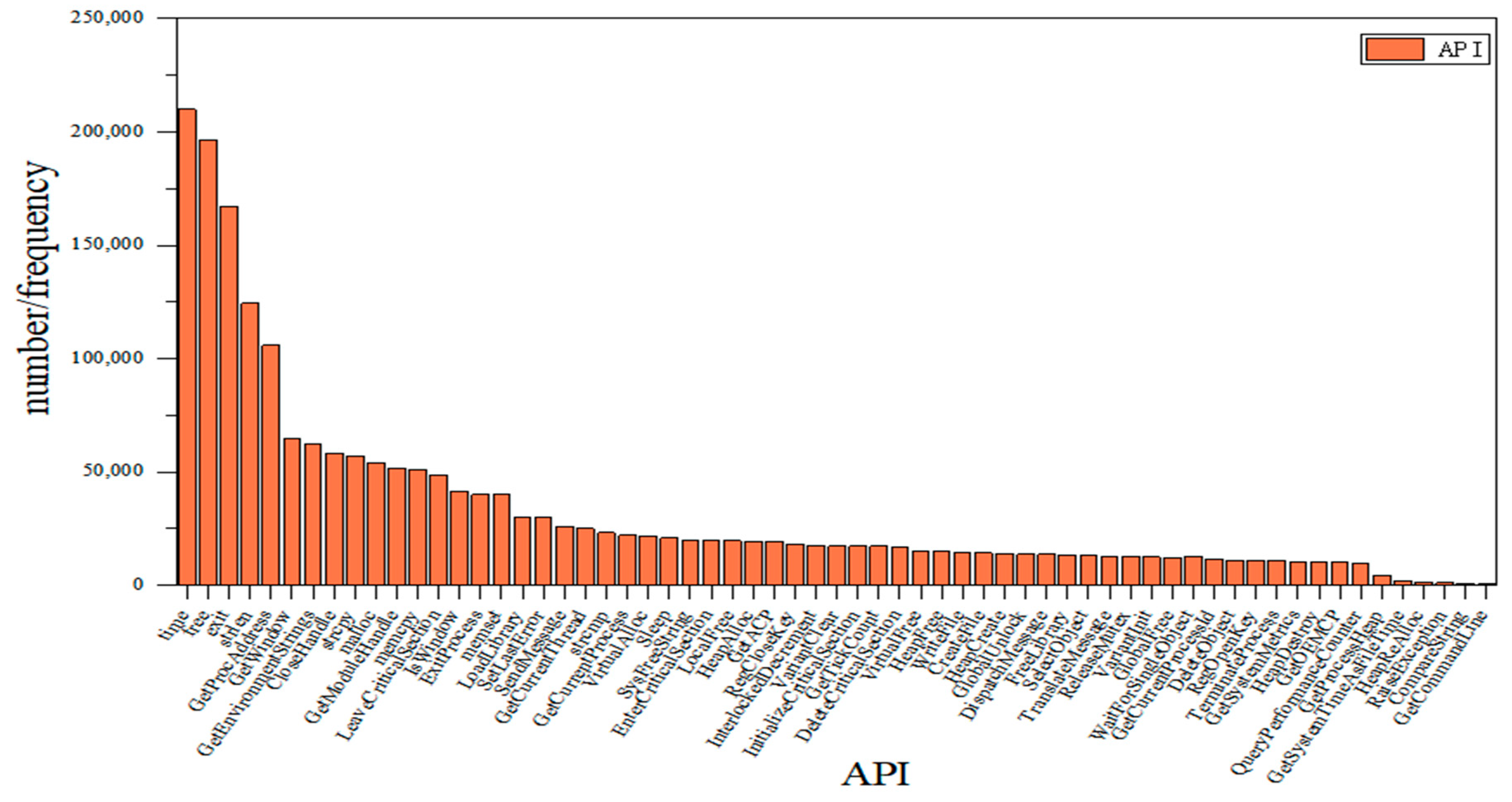
The algorithm is used to analyze the features after the extraction of the training set samples of the dataset, filtering out the redundant samples, keeping the important ones, and simplifying the sample structure. The extracted 1632 Opcodes and 265 APIs were combined and deweighted to rank the importance, and the top 73 Opcodes and 73 API were reweighted to better analyze the influence of Opcode and API on the importance of the model. The results are shown in Figure 7 and Figure 8.
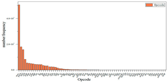
Figure 7.
Ranking Opcode in order of importance.
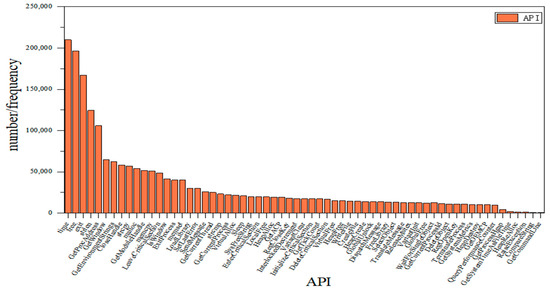
Figure 8.
Ranking API in order of importance.
Figure 7 shows that the most important Opcode feature is “MOV” and the least influential is “LOOP”; similarly, Figure 8 shows that the most important API feature is “time” and “GetCommandLine” is the least influential. At the same time, different features have different importance, and the lower the importance of a feature, the less impact it has on the classification. In this way, invalid features can be filtered to retain the features with high importance and simplify the structure. XGBoost is used in combination with several optimization algorithms to analyze the importance of the features; strongly important features are retained, and redundant features can be filtered out.
In this paper, ref. [30], three optimization algorithms are used to compare. WOA-XGBoost was used to compare the gray wolf optimizer (GWO)-XGBoost, and Bayesian optimization (BO)-XGBoost was used to determine the importance ranking of features and to analyze the detection accuracy of these models. This is shown in Table 3.
Table 3.
Quantity Distribution of Sample DataCon Dataset.
Wasserstein’s algorithm and Spearman’s correlation coefficient were used to analyze the correlation of the features; between features with strong correlation, the remaining features can be removed. The training set samples were extended, and the generated samples were combined with the original samples. The result of this is shown in Figure 9 and Figure 10.
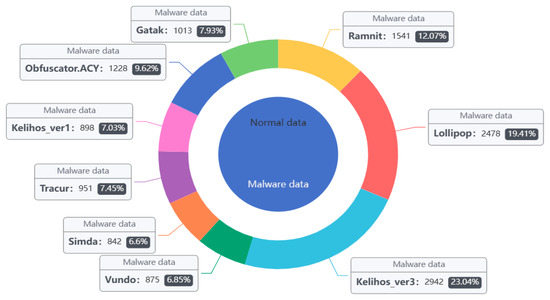
Figure 9.
Sample distribution after Kaggle dataset expansion.

Figure 10.
Sample distribution after DataCon dataset expansion.
In order to fully evaluate our model, experimental comparisons based on different methods were conducted on Kaggle and DataCon datasets. On the basis of the dataset expanded with features based on SFCWGAN, the data were randomly divided into 10 parts using the three-fold cross-validation method, respectively; eight of them were selected as the training set and two as the test set.
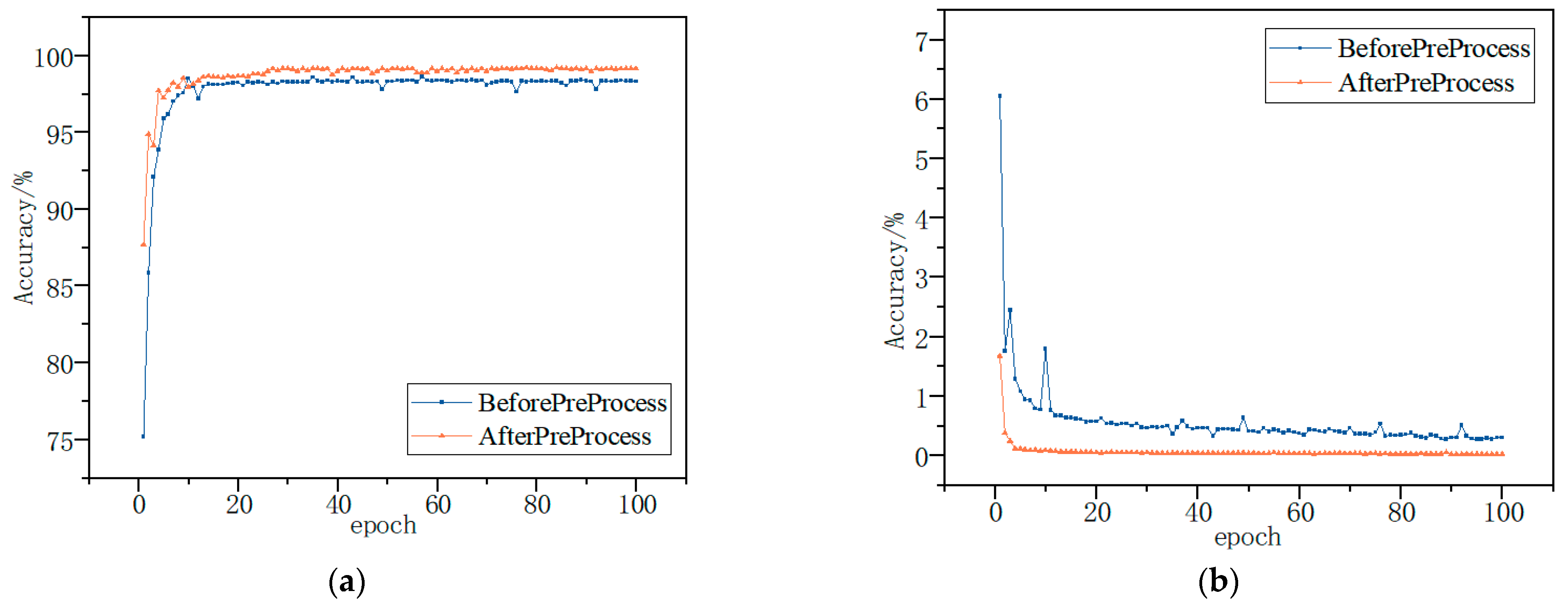
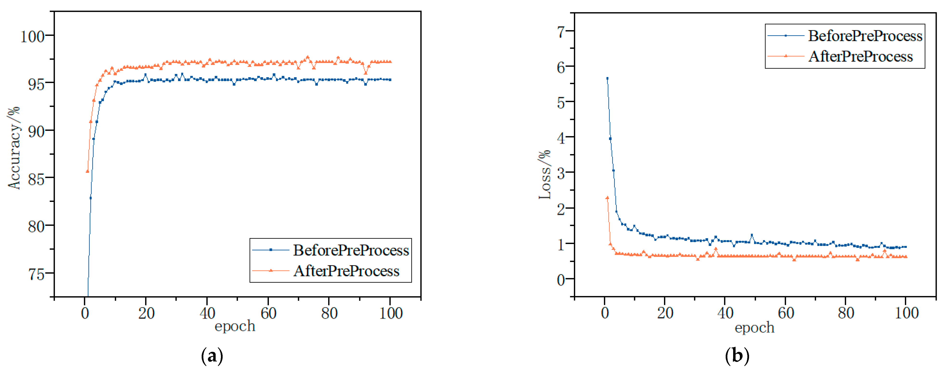
Finally, the BiTCN network was trained using test samples input into the training model, and the detection effectiveness of the model was evaluated by combining the test samples. The trends of the average detection accuracy and loss of the model are shown in Figure 11 and Figure 12. The average accuracy and loss functions of the model converge rapidly and stabilize with the increase in the number of iterations at the processing of the training. The highest accuracies of 99.56% and 96.98% were achieved using the model for multiple classification of the Kaggle and DataCon datasets. The results show that the model is able to identify malware and, thus, has high detection accuracy and good results.
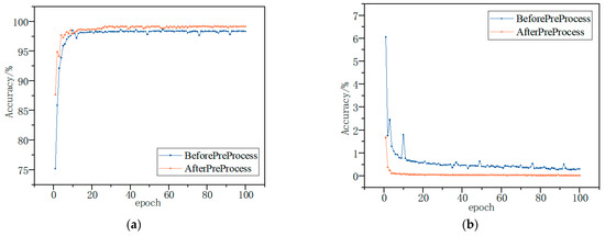
Figure 11.
Kaggle dataset accuracy and loss; they should be listed as: (a) Description of accuracy; (b) Description of loss.
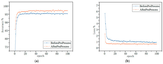
Figure 12.
DataCon dataset accuracy and loss; they should be listed as: (a) Description of accuracy; (b) Description of loss.
It can be seen that by using the features following the Spearman’s correlation coefficient selection, the proposed model is able to accurately classify and detect malware on both datasets, with a significant improvement in accuracy and convergence speed relative to the pre-feature selection. The results show that the use of feature selection can largely mitigate the impact of unbalanced malware family samples, thus improving the final detection accuracy.
4.3.2. Noise Analysis Experiments
In this section, the impact of noise on the model accuracy is verified through the noise robustness experiments of SFCWGAN- and BiTCN-based malware detection methods. Different levels of Gaussian white noise were added to the Kaggle and DataCon datasets, obeying 0.01, 0.03, and 0.05. Table 4 shows the results.
Table 4.
Detection accuracy under the influence of different noise levels.
As can be seen in Table 4, the accuracy of the two datasets is affected to some extent as the noise level increases, but the accuracy reduction level does not exceed 1.4%. The results show that noise has a significant effect on strongly correlated features and a weak effect on weakly correlated features. This indicates that it is not necessary to process all the features and focus on only a few noise-sensitive features. This further demonstrates that the model proposed in this paper performs stably under the influence of noise disturbances, while a small amount of noise has almost no effect.
4.3.3. Comparison of Difference Sample Balance Algorithms
In this session, for the sample imbalance problem, we use the oversampling methods and the GAN to obtain a balanced distribution of data. This paper compares BSO [35], ROS [36], ADASYN [37], SMOTE [7], CWGAN [38], and SFCWGAN methods, which are tested as classifiers for sample balance on the Kaggle and DataCon datasets under the same experimental conditions, and the results are shown in Table 5 and Table 6. In this section, we compare different sample balance algorithms and verify the advantages of the SFCWGAN differential data sample balance algorithm in malware detection. We also compare different sample balance algorithms for the semantic call relationship between API and Opcode and verify the advantages of the SFCWGAN differential data sample balance algorithm for malware detection.
Table 5.
Detection results under the influence of enhanced algorithms on Kaggle dataset.
Table 6.
Detection results under the influence of enhanced algorithms on DataCon dataset.
As can be seen from Table 5 and Table 6, the proposed SFCWGAN-BiTCN achieves the best test results in evaluation Indicators. It can be found that the better performance of this paper’s model in these families, relative to several sample balance methods, is due to the fact that ROS and BOS only resample the sample and both the ADASYN and SMOTE methods do not learn the original features and use the KNN principle for random synthesis of the samples. After comparative analysis, the SFCWGAN captures deep features of the original samples and uses generators in order to generate malware family samples. Compared with the CWGAN, the SFCWGAN increases the feature selection and simplifies the structure. Meanwhile, the combination of Dropout solves the problem of gradient disappearance during the training process, which makes the little malware family samples generated by the SFCWGAN higher-quality and closer to the original samples, and indicates that SFCWGAN is more suitable for mining deep features.
4.3.4. Ablation Experiments
Model ablation experiments were established to validate the impact of the proposed model on the detection ability of a few malware family samples.
The BiTCN, GAN [23]-BiTCN, CWGAN [38]-BiTCN, and the models in this paper were compared on the Kaggle and DataCon datasets under the same experimental conditions. The traditional algorithms performed poorly for Vundo, Simda, Tracur and Kelihos_ver1, which are families. Among them, for the Simda family with only 42 samples, the classification accuracy was poor, mainly because the sample size was too small to obtain accurate family features. The accuracy for each model was evaluated for difference malware families of the Kaggle and DataCon datasets and are shown in Table 7 and Table 8.
Table 7.
Accuracy of different GANs on Kaggle Dataset.
Table 8.
Accuracy of different GANs on DataCon Dataset.
As can be seen from Table 7 and Table 8, the accuracy of the unbalanced malware family samples based on feature selection and this paper’s model is significantly improved. The main reason is that the actual samples include many invalid features, and using feature selection to remove redundant features simplifies the structure and improves the accuracy. The GAN, CWGAN, and SFCWGAN were used with sample expansion for the families Vundo, Simda, Tracur, and Kelihos_ver1. By combining with the original training set, the unbalanced malware family samples are increased to expand the malware family samples and solve the gradient disappearance problem. The results show that the model generates samples that address the malware family imbalance problem, thus improving the overall detection accuracy.
4.3.5. Comparison of Difference Classification Algorithms
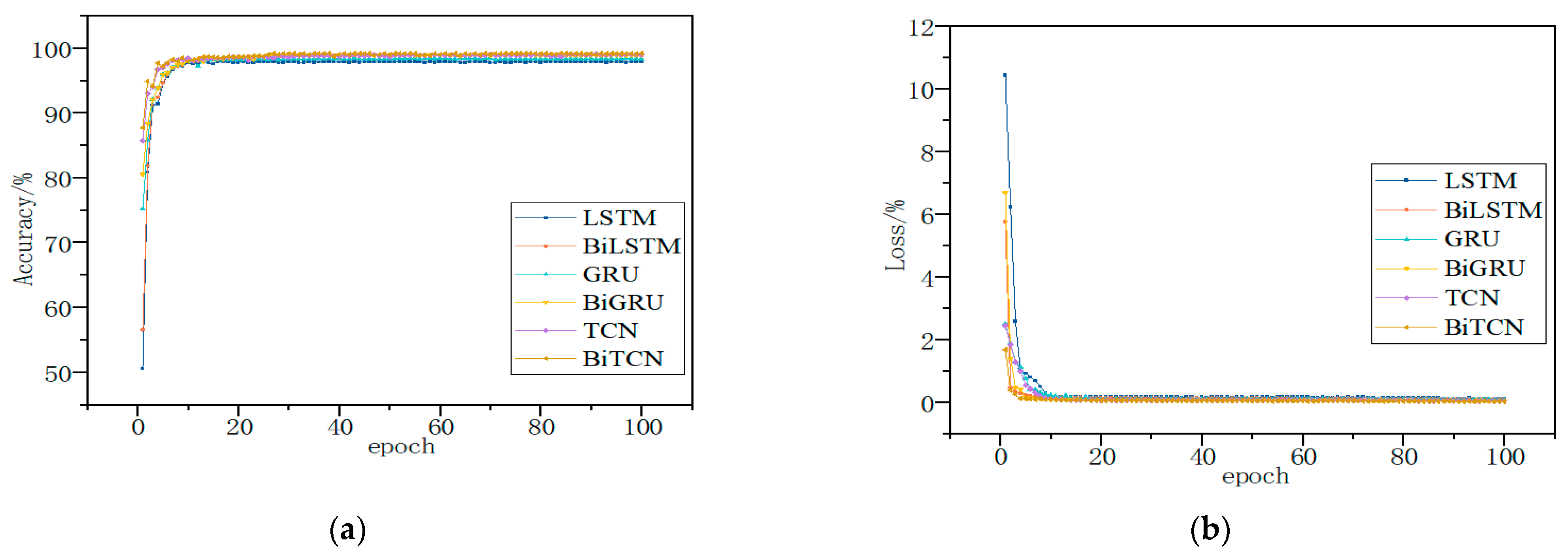
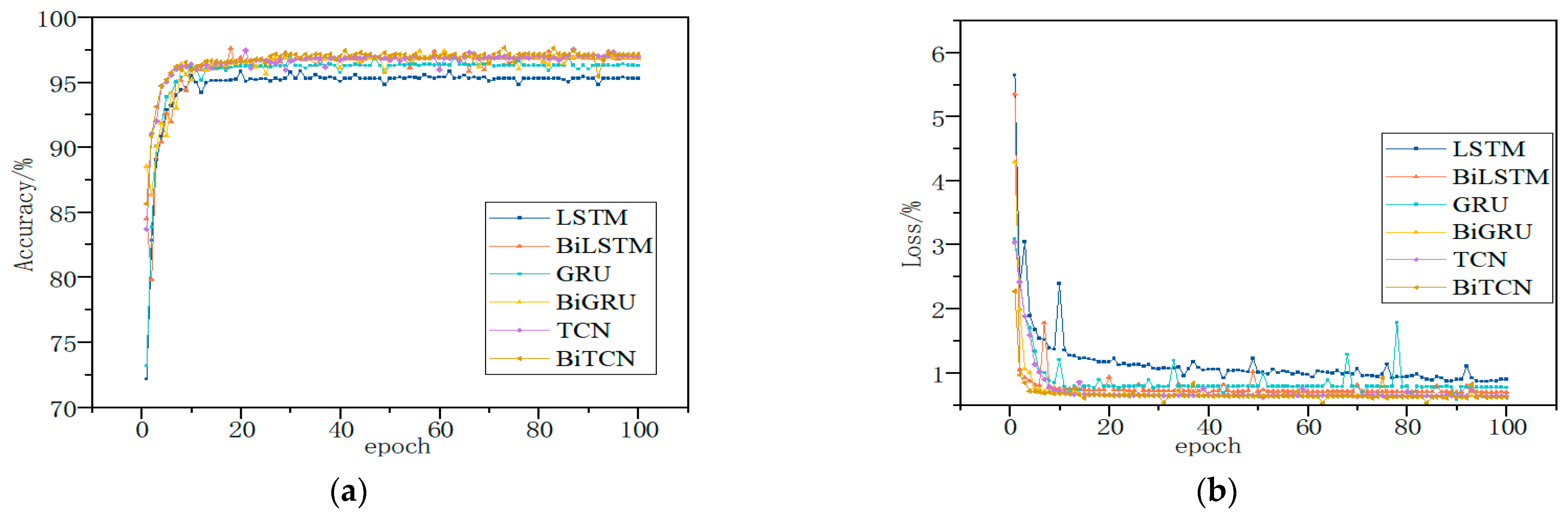
Through comparative experiments, it was verified that BiTCN achieved better results in malware classification. The dataset was processed using the SFCWGAN under the same experimental conditions and then trained on a long short-term memory network (LSTM), bidirectional long short-term memory network (BiLSTM) [39], gated recurrent unit (GRU), bidirectional gated recurrent unit (BiGRU) [40], TCN and BiTCN. The results of different algorithms for malware behavior analysis are shown in Table 9 and Table 10 and Figure 13 and Figure 14.
Table 9.
Detection accuracy under the influence of difference algorithms on Kaggle dataset.
Table 10.
Detection accuracy under the influence of difference algorithms on DataCon dataset.
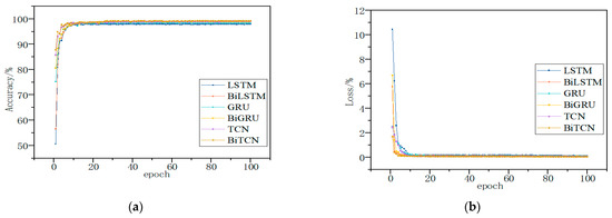
Figure 13.
The Evaluation Results Based on Kaggle Dataset; they should be listed as: (a) Description of accuracy; (b) Description of loss.
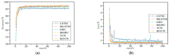
Figure 14.
The Evaluation Results Based on DataCon Dataset; they should be listed as: (a) Description of accuracy; (b) Description of loss.
The sequence features of malware have obvious temporal characteristics, and the TCN has a strong capability to process time series, which can perform deeper feature extraction on the sequence data. Therefore, the method can achieve better results in malware detection. The TCN can only read sequence features from one direction and cannot mine the inverse sequence features. Therefore, end-to-end fusion of TCNs is performed to form BiTCN models for processing temporal features to improve detection accuracy.
4.3.6. Comparison of Existing Methods
We compared with existing methods in order to further validate the performance of the SFCWGAN- and BiTCN-based malware detection algorithms. Those were applied to the Kaggle and DataCon datasets according to their published descriptions and parameter settings, and yielded the results shown in Table 11.
Table 11.
Detection accuracy under the influence of difference algorithms on Kaggle dataset.
Jha et al. [21] use a LeNet5 structure based on the Word2Vec multi-channel feature matrix. Due to the diversity and polymorphism of malicious code, the code structure of malware can change significantly, making the model difficult to converge and less accurate. Gibert et al. [20] use grayscale images as features and do not take into account the semantic features of binary code, resulting in lower accuracy. Gibert et al. [41] feature byte sequences, API function calls, and Opcodes using a LeNet5 structure based on the Word2Vec multichannel feature matrix but with different colors for different features, which ignores correlation between features. Yan et al. [42] extract features via a CNN model for grayscale maps and LSTM model for Opcode features, then fuse the results for classification. The extracted image features are trained using ResNet and GoogleNet models. N. Marastoni et al. [43] uses CNN and LSTM models, respectively, to classify malware image features using migration learning methods. Darem et al. [44] propose an approach with integrated deep learning, feature engineering, image transformation, and processing techniques, and use CNN and XGBoost methods. Lin and Yeh’s [45] one-dimensional convolutional neural networks (CNNs) are presented in order to detect and classify malware families. Chen et al.’s work [46] proposes different malware detection techniques based on CNN, LSTM, and bidirectional LSTM models. These models were trained on raw API sequences and parameters traced during the execution of malware and benign executable files.
These methods did not perform as well as expected for Vundo, Simda, Tracur, and Kelihos_ver1, which are families. In particular, for the Simda family with only 42 samples, the classification accuracy was only 85.92%, mainly because the sample size was too small to obtain accurate family features. Compared these methods, our model uses the SFCWGAN to simplify the feature structure, continues to expand on a few malware family samples, and reduces the impact of malware family sample imbalance, resulting in better detection results. The model uses the BiTCN for feature extraction and classification to extract deeper and more deep-level features from the time series level, resulting in better detection results.
5. Conclusions
To address the problem of imbalanced malware family samples on malware detection models, this paper proposes a malware detection method based on the SFCWGAN and BiTCN, which can improve effectiveness and accuracy in detecting malware. The samples were pre-processed using WOA-XGBoost and Spearman’s correlation coefficients to simplify the feature structure by removing redundant features. A few malware family samples were generated using the CWGAN to complement the dataset and mitigate the malware family imbalance. Feature vectors of malware API and Opcode call sequences were constructed via Word2Vec representation, combined with BiTCN to highlight the semantic associations between API and Opcode calls. Experiments of the model on Kaggle and DataCon datasets demonstrate improved detection capability for a few malware family samples. It has powerful feature extraction capability and high accuracy when dealing with large-scale malware samples and shows good results in malware detection based on existing network captures.
However, the accuracy and bias of this model on the DataCon dataset suggests that there is room for improvement and minimal bias. Future work will focus on this deficiency, and we will investigate the construction of feature extraction and classification models to find ways to improve detection accuracy and minimize the bias. Notably, malware has become one of the most serious security threats to the IoT. The application of malware variant classification in IoT needs to be explored further for a series of problems caused by the propagation of malware codes from traditional networks to IoT and within IoT.
Author Contributions
B.X.: conceptualization, methodology, writing—original draft; J.L.: formal analysis, writing—review and editing; Y.S.: conceptualization, formal analysis, methodology, funding acquisition. All authors have read and agreed to the published version of the manuscript.
Funding
This work is supported by the National Science Foundation of China (61806219, 61703426 and 61876189), by the National Science Foundation of Shaanxi Provence (2021JM-226), by the Young Talent fund of University and Association for Science and Technology in Shaanxi, China (20190108, 20220106), and by and the Innovation Capability Support Plan of Shaanxi, China (2020KJXX-065).
Institutional Review Board Statement
Not applicable.
Informed Consent Statement
Not applicable.
Data Availability Statement
All data used in this paper can be obtained by contacting the authors of this study.
Conflicts of Interest
The authors declare no conflict of interest.
References
- Kim, S.; Hong, S.; Oh, J. Obfuscated VBA macro detection using machine learning. In Proceedings of the 2018 48th Annual IEEE/IFIP International Conference on Dependable Systems and Networks (DSN), Luxembourg, 25–28 June 2018; pp. 490–501. [Google Scholar]
- Wang, S.; Chen, Z.; Yan, Q. Deep and broad URL feature mining for android malware detection. Inf. Sci. 2020, 513, 600–613. [Google Scholar] [CrossRef]
- Demetrio, L.; Coull, S.E.; Biggio, B. Adversarial exemples: A survey and experimental evaluation of practical attacks on machine learning for windows malware detection. ACM Trans. Priv. Secur. 2021, 24, 1–31. [Google Scholar] [CrossRef]
- Li, D.; Li, Q.; Ye, Y. Arms race in adversarial malware detection: A survey. ACM Comput. Surv. 2021, 55, 1–35. [Google Scholar] [CrossRef]
- Mimura, M.; Ohminami, T. Using LSI to detect unknown malicious VBA macros. J. Inf. Process. 2020, 28, 493–501. [Google Scholar] [CrossRef]
- Mimura, M. Using fake text vectors to improve the sensitivity of minority class for macro malware detection. J. Inf. Secur. Appl. 2020, 54, 102600. [Google Scholar] [CrossRef]
- Chawla, N.V.; Bowyer, K.W.; Hall, L.O. SMOTE: Synthetic minority over-sampling technique. J. Artif. Intell. Res. 2002, 16, 321–357. [Google Scholar] [CrossRef]
- Bunkhumpornpa, C.; Sinapiromsaran, K.; Lursinsap, C. Safe-level-smote: Safe-level-synthetic minority over-sampling technique for handling the class imbalanced problem. In Proceedings of the Pacific-Asia Conference on Knowledge Discovery and Data Mining, Bangkok, Thailand, 27–30 April 2009; pp. 475–482. [Google Scholar]
- Graa, O.; Rekik, I. Multi-view learning-based data proliferator for boosting classification using highly imbalanced classes. J. Neurosci. Methods 2019, 327, 108344. [Google Scholar] [CrossRef]
- Fu, G.H.; Wu, Y.J.; Zong, M.J. Hellinger distance-based stable sparse feature selection for high-dimensional class-imbalanced data. BMC Bioinform. 2020, 21, 1–14. [Google Scholar] [CrossRef]
- Cui, Z.; Xue, F.; Cai, X. Detection of malicious code variants based on deep learning. IEEE Trans. Ind. Inform. 2018, 14, 3187–3196. [Google Scholar] [CrossRef]
- Goodfellow, I.; Pouget-Abadie, J.; Mirza, M. Generative adversarial networks. Commun. ACM 2020, 63, 139–144. [Google Scholar] [CrossRef]
- Kim, J.Y.; Bu, S.J.; Cho, S.B. Malware detection using deep transferred generative adversarial networks. In Proceedings of the 2017 International Conference on Neural Information Processing, Long Beach, CA, USA, 4–9 December 2017; pp. 556–564. [Google Scholar]
- Kim, J.Y.; Bu, S.J.; Cho, S.B. Zero-day malware detection using transferred generative adversarial networks based on deep autoencoders. Inf. Sci. 2018, 460, 83–102. [Google Scholar] [CrossRef]
- Liu, Y.; Li, J.; Liu, B. Malware detection method based on image analysis and generative adversarial networks. Concurr. Comput.: Pract. Exp. 2022, 34, e7170. [Google Scholar] [CrossRef]
- Suciu, O.; Coull, S.E.; Johns, J. Exploring adversarial examples in malware detection. In Proceedings of the 2019 IEEE Security and Privacy Workshops (SPW), San Francisco, CA, USA, 19–23 May 2019; pp. 8–14. [Google Scholar]
- Hu, W.; Tan, Y. Generating adversarial malware examples for black-box attacks based on GAN. Comput. Sci. 2017, 99, 8–14. [Google Scholar]
- Tang, C.; Zhang, Y.; Yang, Y.X. DroidGAN: Android adver sarial sample generation framework based on DCGAN. J. Commun. 2018, 39, 64–69. (In Chinese) [Google Scholar]
- Rosenberg, I.; Shabtai, A.; Rokach, L. Generic black-box end-to-end attack against state of the art API call based malware classifiers. In Proceedings of the 2018 International Symposium on Research in Attacks, Intrusions, and Defenses, Crete, Greece, 10–12 September 2018; pp. 490–510. [Google Scholar]
- Jha, S.; Prashar, D.; Long, H.V. Recurrent neural network for detecting malware. Comput. Secur. 2020, 99, 102037. [Google Scholar] [CrossRef]
- Gibert, D.; Mateu, C.; Planes, J. HYDRA: A multimodal deep learning framework for malware classification. Comput. Secur. 2020, 95, 101873. [Google Scholar] [CrossRef]
- Yu, L.; Zhang, W.; Wang, J. Seqgan: Sequence generative adversarial nets with policy gradient. In Proceedings of the AAAI Conference on Artificial Intelligence, San Francisco, CA, USA, 4–9 February 2017; pp. 23–30. [Google Scholar]
- Liao, D.; Huang, S.; Tan, Y. Network intrusion detection method based on gan model. In Proceedings of the 2020 International Conference on Computer Communication and Network Security (CCNS), Xi’an, China, 21–23 August 2020; pp. 153–156. [Google Scholar]
- Huang, S.; Lei, K. IGAN-IDS: An imbalanced generative adversarial network towards intrusion detection system in ad-hoc networks. Ad Hoc Netw. 2020, 105, 102177. [Google Scholar] [CrossRef]
- Solis, D.; Vicens, R. Convolutional neural networks for classification of malware assembly code. In Proceedings of the 20th International Conference of the Catalan Association for Artificial Intelligence, Terres de L’Ebre, Spain, 25–27 October 2017. [Google Scholar]
- McLaughlin, N.; Martinez del Rincon, J.; Kang, B.J. Deep android malware detection. In Proceedings of the Seventh ACM on Conference on Data and Application Security and Privacy, Scottsdale, AZ, USA, 22–24 March 2017; pp. 301–308. [Google Scholar]
- Bhati, B.S.; Chugh, G.; Al-Turjman, F. An improved ensemble based intrusion detection technique using XGBoost. Trans. Emerg. Telecommun. Technol. 2021, 32, e4076. [Google Scholar] [CrossRef]
- Ikram, S.T.; Cherukuri, A.K.; Poorva, B. Anomaly detection using XGBoost ensemble of deep neural network models. Cybern. Inf. Technol. 2021, 21, 175–188. [Google Scholar] [CrossRef]
- Mirjalili, S.; Lewis, A. The whale optimization algorithm. Adv. Eng. Softw. 2016, 95, 51–67. [Google Scholar] [CrossRef]
- Qiu, Y.; Zhou, J.; Khandelwal, M. Performance evaluation of hybrid WOA-XGBoost, GWO-XGBoost and BO-XGBoost models to predict blast-induced ground vibration. Eng. Comput. 2021, 1–18. [Google Scholar] [CrossRef]
- Mirjalili, S.; Mirjalili, S.M.; Hatamlou, A. Multi-verse optimizer: A nature-inspired algorithm for global optimization. Neural Comput. Appl. 2016, 27, 495–513. [Google Scholar] [CrossRef]
- Dubey, G.P.; Bhujade, R.K. Optimal feature selection for machine learning based intrusion detection system by exploiting attribute dependence. Mater. Today Proc. 2021, 47, 6325–6331. [Google Scholar] [CrossRef]
- Ronen, R.; Radu, M.; Feuerstein, C. Microsoft Malware Classification Challenge 2018. Comput. Secur. 2020, 95, 101873. Available online: https://www.kaggle.com/c/malware-classification/data (accessed on 28 December 2022).
- Qi An Xin Technology Research Institute. DataCon: Multidomain Large-Scale Competition Open Data for Security Research. Available online: https://datacon.qianxin.com/opendata (accessed on 11 November 2021). (In Chinese).
- Han, H.; Wang, W.Y.; Mao, B.H. Borderline-SMOTE: A new over-sampling method in imbalanced data sets learning. In Proceedings of the International Conference on Intelligent Computing, Hefei, China, 23–26 August 2005; pp. 878–887. [Google Scholar]
- Mease, D.; Wyner, A.J.; Buja, A. Boosted classification trees and class probability/quantile estimation. J. Mach. Learn. Res. 2007, 8. [Google Scholar]
- He, H.; Bai, Y.; Garcia, E.A. ADASYN: Adaptive synthetic sampling approach for imbalanced learning. In Proceedings of the 2008 IEEE International Joint Conference on Neural Networks (IEEE World Congress on Computational Intelligence), Hong Kong, China, 1–6 June 2008; pp. 1322–1328. [Google Scholar]
- Yu, Y.; Tang, B.; Lin, R. CWGAN: Conditional wasserstein generative adversarial nets for fault data generation. In Proceedings of the 2019 IEEE International Conference on Robotics and Biomimetics (ROBIO), Dali, China, 6–8 December 2019; pp. 2713–2718. [Google Scholar]
- Lu, W.; Li, J.; Wang, J. A CNN-BiLSTM-AM method for stock price prediction. Neural Comput. Appl. 2021, 33, 4741–4753. [Google Scholar] [CrossRef]
- She, D.; Jia, M. A BiGRU method for remaining useful life prediction of machinery. Measurement 2021, 167, 108277. [Google Scholar] [CrossRef]
- Gibert, D.; Mateu, C.; Planes, J. Orthrus: A Bimodal Learning Architecture for Malware Classification. In Proceedings of the 2020 International Joint Conference on Neural Networks (IJCNN), Glasgow, UK, 19–24 July 2020; pp. 1–8. [Google Scholar]
- Yan, J.; Qi, Y.; Rao, Q. Detecting malware with an ensemble method based on deep neural network. Secur. Commun. Netw. 2018, 2018, 7247095. [Google Scholar] [CrossRef]
- Marastoni, N.; Giacobazzi, R.; Dalla, P.M. Data augmentation and transfer learning to classify malware images in a deep learning context. J. Comput. Virol. Hacking Tech. 2021, 17, 279–297. [Google Scholar] [CrossRef]
- Darem, A.; Abawajy, J.; Makkar, A. Visualization and deep-learning-based malware variant detection using OpCode-level features. Future Gener. Comput. Syst. 2021, 125, 314–323. [Google Scholar] [CrossRef]
- Lin, W.C.; Yeh, Y.R. Efficient Malware Classification by Binary Sequences with One-Dimensional Convolutional Neural Networks. Mathematics 2022, 10, 608. [Google Scholar] [CrossRef]
- Chen, X.; Hao, Z.; Li, L. CruParamer: Learning on Parameter-Augmented API Sequences for Malware Detection. IEEE Trans. Inf. Forensics Secur. 2022, 17, 788–803. [Google Scholar] [CrossRef]


Disclaimer/Publisher’s Note: The statements, opinions and data contained in all publications are solely those of the individual author(s) and contributor(s) and not of MDPI and/or the editor(s). MDPI and/or the editor(s) disclaim responsibility for any injury to people or property resulting from any ideas, methods, instructions or products referred to in the content. |
© 2023 by the authors. Licensee MDPI, Basel, Switzerland. This article is an open access article distributed under the terms and conditions of the Creative Commons Attribution (CC BY) license (https://creativecommons.org/licenses/by/4.0/).