1. Introduction
Automation of the process of determining Surface Vehicle (SV) position coordinates in the coastal zone using radar, Light Detection And Ranging (LiDAR) or Charge-Coupled Device (CCD), and Complementary Metal-Oxide-Semiconductor (CMOS) cameras is currently the subject of much research [
1,
2,
3,
4,
5,
6,
7,
8,
9,
10]. Much of it is directed towards developing algorithms for coordinate position estimation using the Extended Kalman Filter (EKF) in its classical form or its modified versions: Unscented Kalman Filter (UKF), Particle Filter (PF), Central Difference Kalman Filter (CDKF) [
11,
12,
13,
14,
15,
16,
17,
18,
19], adaptive fault-tolerant extended Kalman filter (AFTKEF) [
20], and resilient extended Kalman filter [
21]. The last two of the mentioned algorithms work well in the case of partial loss of data from sensors—“input”. The idea of the AFTEKF algorithm is to choose a suitable so-called fading factor based on the orthogonal theory and embed it into the prior state covariance matrix. The resilient extended Kalman filter is proposed for discrete-time nonlinear stochastic systems with sensor failures and random observer gain perturbations. Resilient extended Kalman filter is intended for discrete-time nonlinear stochastic systems with sensor failures and random observer gain perturbations. During his work, he assumes that the failure mechanisms of multiple sensors are independent of each other, with different failure rates. The locally unbiased robust minimum mean square filter is designed for state estimation under these conditions.
In the case of SV positioning, the EKF input provides both parameters describing the SV’s movement vector (e.g., course and speed)—determined, for example, by Doppler Velocity Log (DVL) and Fibre-Optic Gyroscope (FOG)—as well as the results from measurements (distances and bearings) taken relative to beacons with known positions (obtained, for example, from an electronic navigation chart)—determined, for instance, by radar or LiDAR, or by the camera.
The EKF works perfectly when there is a misidentification of beacons, leading to the assignment of converted measurement results [
3]. The algorithm treats such measurement results as having a gross error and, as a result, suppresses them. In particular, this problem may arise when the beacons are located very close to each other or when the movement of the SV from which the measurements are taken is disturbed (i.e., the SV tilts, causing uncontrolled changes in course and speed).
However, several position coordinate estimation methods have also been developed in the field of surveying that can detect, suppress, and eliminate gross error measurements [
22,
23,
24,
25,
26]. The best known and considered among the best are methods based on the so-called equivalent weight matrix. Of these, Hampel’s Geodetic Robust Adjustment (GRA) and Danish methods are the most widely used [
25,
26].
However, there is an essential difference between EKF and GRA, regarding how gross error measurements are suppressed. EKF uses a gain matrix for this purpose, taking into account the historical covariance matrix. GRA, on the other hand, uses a covariance matrix built continuously, and considers the equivalent weighting matrix.
For these reasons, the accuracy of position coordinate estimation by these methods can be expected to depend to varying degrees on the number and type of measurements, the way the beacons are positioned relative to each other, and the position relative to the SV beacons.
A study is therefore warranted to allow a comparative assessment of the two methods. Since EKF is used for positioning in dynamics and GRA for positioning in statics, this type of research is not likely to be found in the literature. For these reasons, it is expected that their results may be unique, but they can indeed find their practical application in specific measurement conditions.
This article presents research into the potential for improving surface vehicle positioning accuracy through the interchangeable use of GRA and EKF methods. It is divided into four sections. The second section formulates a scientific problem related to the positioning accuracy of SV with the selected methods based on measurements made with onboard navigation equipment and a measurement system based on an omnidirectional camera. The third section describes a simulation study involving the generation of navigational measurement results with errors (including gross errors). The method is used to position an SV sailing along a given trajectory in the vicinity of three beacons. The fourth section presents an extensive analysis of the simulation results, indicating that the GRA and EKF methods as the best for positioning the SV. It provides a proposal for the index to select the most accurate one under specific measurement conditions. The final section provides generalised conclusions from the study and guidance on the interchangeable use of EKF and GRA methods.
2. Problem Formulation
Let SV be in motion (swims along a given trajectory) in the time interval . During this time, at any moment , the onboard navigation equipment determines course over ground and speed over ground . The measuring system is based on an omnidirectional camera, which determines relative bearings and distances to n beacons, located in the navigation area.
At each subsequent moment
, based on the results of the measurements
and
taken at the previous moment instant
, let the so-called state vector be estimated:
. This is done using a function for a non-linear SV motion model (DR method) (
1).
where:
—coordinates of the SV position calculated at the moment k,
—time period from k to time moments,
, —are known control inputs at k time moment,
—so-called random disturbances in the determination of coordinates, course over ground and speed over ground in the form of errors with zero expectation value and normal distribution at k time moment.
In addition, based on the estimated state vector
and the known coordinates of
of the position of the
i-th beacon
, let the observation vector be estimated
(distance and relative bearing to the beacon
) using the function (
2):
where:
i-th navigational mark against which measurements have been taken and is measured using the system based on the omnidirectional camera at the moment ;
— of the SV expressed in semicircular measure, as determined by onboard navigational equipment at the moment ;
—so-called random distortions in the determination of the distance and relative bearing to the i-th navigational mark, expressed in terms of errors with zero expectation and normal distribution at the moment .
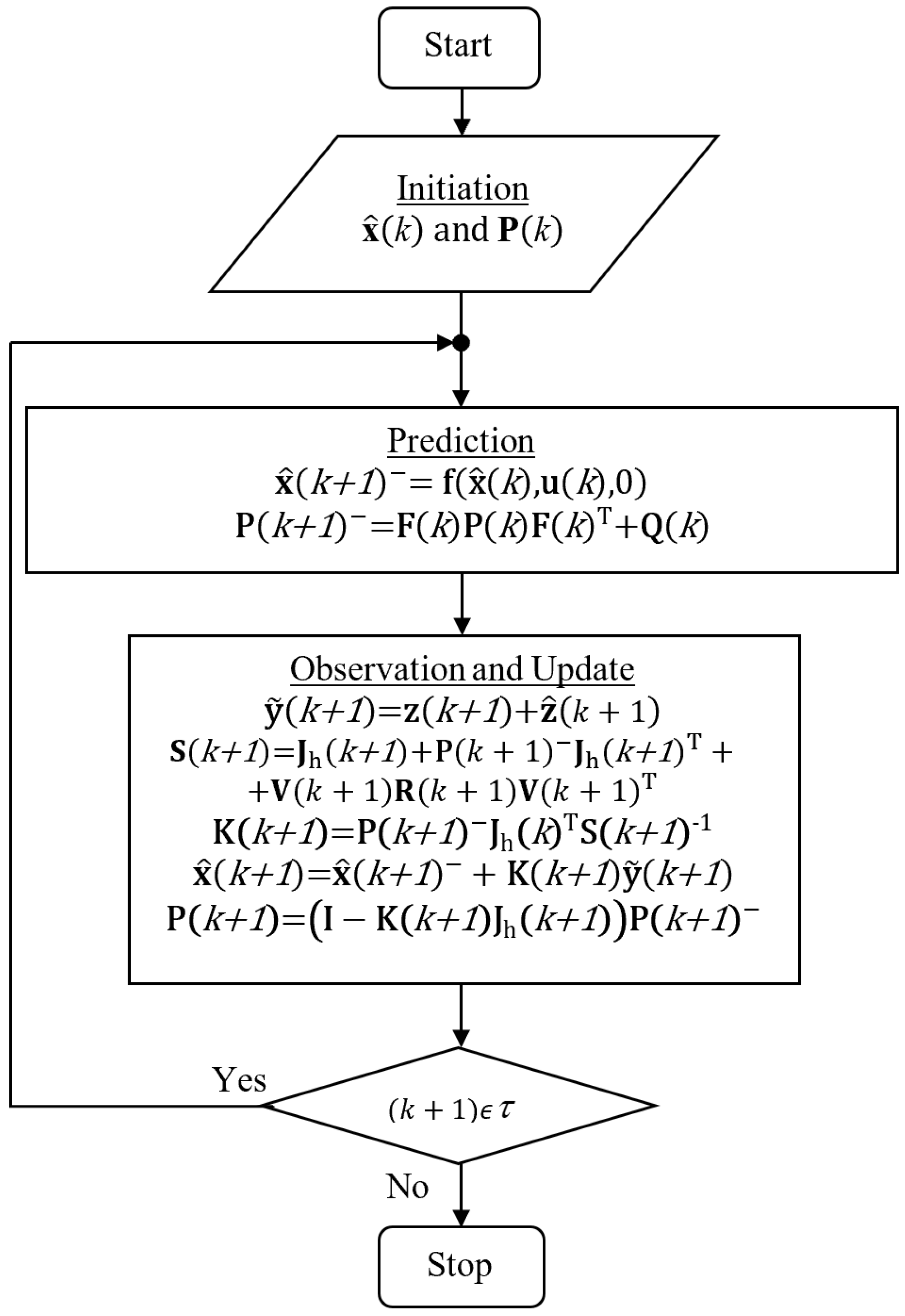
The functions, constructed as
and
, can be used to estimate SV position coordinates according to the EKF algorithm from both measurements
and
, as well as
and
(
Figure 1).
Figure 1.
Algorithm of the estimation of the vector state using Extended Kalman Filter.
Figure 1.
Algorithm of the estimation of the vector state using Extended Kalman Filter.
where:
and —the estimated state vector and its covariance matrix, fixed a posteriori at time moment ,
and —the estimated state vector and its covariance matrix, fixed a priori at time moment ,
—the so-called system matrix calculated as a Jacobi matrix of functions ,
—the noise matrix of state vector at the time of moment k for assumed mean error values of the following measurements: course over ground and speed over ground , where:
,
,
,
—of the state vector updated in the next time moment k,
—the Jacobi matrix of the function , generated for each pair of measurements taken up to the i-th navigation mark, with ,
,
,
—the noise matrix of a vector of instantaneous observations with the assumed values of the mean errors of the distance and relative bearing measurements and bearing to the beacons.
The SV position coordinates can also be estimated without measurement
, i.e., based on measurement results
,
and
. For this purpose, the classical geodetic adjustment method using the least squares method (GLSA) or the robust adjustment method (GRA), based on the so-called equivalent weighting matrix of measurements with gross error, can be used. The functional and stochastic models and the optimisation criteria for the two indicated geodetic adjustment methods could be formulated as follows [
25,
26,
27]:
Given the assumptions (Equation (3)), after appropriate mathematical transformations, Relations
4 and
5 can be created for the estimation of the correction vector
of the predicted coordinates of the SV position (state vector
, established a priori):
where:
—design matrix,
—residual vector,
—variance coefficient,
—equivalent weighting matrix,
—diagonal damping matrix,
—Danish damping function, where:
and —parameters controlling the gross error measurement weights,
—covariance matrix for ,
,
—weight matrix.
Based on Formulae (
4) and (
5) obtained in this way, it is possible to estimate the state vector iteratively
at each successive moment
, according to the algorithm shown in
Figure 2 for the GLSA method, and according to the algorithm shown in
Figure 3 for the GRA method. By starting the iterative computation process after the prediction has been performed, the process can be considered to be complete when the absolute values of the differences of the correction vectors
will be smaller than the maximum absolute values of the vector correction increments
.
Assume that the calculations for values are determined arbitrarily at the time of initialisation of the algorithms, while the values are determined after each successive prediction.
Figure 2.
Algorithm for state vector estimation using classical geodetic adjustment.
Figure 2.
Algorithm for state vector estimation using classical geodetic adjustment.
Let us now assume that, based on the results of the measurements
and
obtained using SV’s onboard navigation equipment, e.g., the Inertial Navigation System (INS) from VectorNav ‘NS-100’ [
28] and the Doppler Velocity Log (DVL) from LinkQuest ‘NavQuest 600’ [
29] (ignoring the effects of current and sea drift), at any time moment
, during the time interval
, the DR method
1 is used to determine the position coordinate vector
.
Knowing the covariance matrix
of the initial (previous) position coordinate vector
and the covariance matrix
of the coordinate vector increment
, it is possible to calculate the covariance matrix
of the coordinate vector of the final (next) position
according to the relation:
In turn, the covariance matrix obtained in this way, , can be used indirectly to assess the accuracy of the position vector determination, , carried out with the following:
Mean ellipse error
where:
,
—directional angle of the ellipse;
a—length of the large half-axis of the ellipse;
b—length of the small half-axis of the ellipse.
Figure 3.
Algorithm for state vector estimation using geodetic adjustment with Danish gross error suppression function.
Figure 3.
Algorithm for state vector estimation using geodetic adjustment with Danish gross error suppression function.
Knowing the values of the measurement errors (
and
) of the measured speed given by the manufacturers of INS ‘NS-100’ and DVL ‘NavQuest 600’ in the technical specifications [
28,
29] and assuming that the SV flows with uniform rectilinear motion
and
, the positions of circles of mean error (having radius length equal to
) and mean error ellipses (having semi-axis lengths equal to
a and
b, and a directional angle equal to
) of the positions determined by the DR method, e.g., after 200 s and after 500 s (which are illustrated in
Figure 4), can be calculated.
Figure 4.
Change in mean error and mean error ellipse after SV travels 1200 m and 3000 m.
Figure 4.
Change in mean error and mean error ellipse after SV travels 1200 m and 3000 m.
Figure 4 shows that the mean error ellipse extends in the direction perpendicular to the
. Its half-axis length
b is almost twice as short as the half-axis
a. Thus, it is the measurement error
which determines the mean error
, whose value reaches 108.9 m after the SV has travelled a distance of only 3000 m.
Let us also assume that the SV can, at any subsequent time
, determine the coordinates of the occupied positions. This is also done using the GLSA method (
Figure 2), solely based on course over ground measurements
performed by, e.g., GNSS Satellite Compass ComNav [
30], and relative bearings
and distances
taken, e.g., with an omnidirectional camera relative to the three navigation marks. The mean error values of the positions determined in this way can then be calculated from the trace of the covariance matrix according to the formula:
where:
assuming that
.
Figure 5 shows the areas of the accuracy of GLSA-determined positions relative to three beacons set in two characteristic variants.
Moreover,
Figure 5 shows that the two variants of beacon alignment (a) and (b) allow the GLSA method to determine position with a mean error of less than the 30 m level in many of the drawn areas of accuracy. This means that the GLSA method can outperform the DR method in terms of the accuracy of the SV position determination. This situation may occur in the case of continuous position determination by the DR method after exceeding the contractual time limit, depending on the values of
and
. Taking into account the results of the calculation of the positioning accuracy with the DR method presented in
Figure 4, it can be stated, with certainty, that the contractual limit was already exceeded after 120 s. At this point, the mean error
reached a value of 43.6 m.
Figure 5.
Position accuracy areas are determined by the GLSA method based on relative bearings and distances taken relative to three navigation marks aligned: (
a) in a line, (
b) in a triangle. (
—arbitrarily assumed,
—assumed based on [
30]; the distance between beacons is approximately 2600 m).
Figure 5.
Position accuracy areas are determined by the GLSA method based on relative bearings and distances taken relative to three navigation marks aligned: (
a) in a line, (
b) in a triangle. (
—arbitrarily assumed,
—assumed based on [
30]; the distance between beacons is approximately 2600 m).
Mainly for these reasons, the augmented Kalman filter method is now often used to determine SV positions. In its operation, it can make use of both measurements of motion parameters , , as well as additional measurements of relative bearings .
However, it is essential to realise that the EKF is a good solution when the measurement error values are set ’perfectly’. Unfortunately, the movement of the SV is almost always disturbed by wind, sea currents, and wave action. Under their influence, the SV hull tilts uncontrollably, changing course and speed; consequently, this leads to high variability in measurement accuracy. In particular, this problem can be attributed to the data-processing specificity of camera measurements taken against land and floating beacons.
At this point, therefore, two questions of scientific interest can be asked regarding the choice of method for determining SV positions:
Must the accuracy of EKF position determination always be greater than the accuracy of GLSA or GRA position determination?
If the answer to the first question is no, in which situations can GLSA or GRA be indicated as a better method for determining positions. In which cases will an extended Kalman filter be better?
The article’s authors will attempt to answer the questions thusly posed in a later section. The results of simulation studies will be helpful for this purpose. These will consist of generating measurement results with errors (including gross errors), and then, estimating position coordinates on their basis using the extended Kalman filter method (according to the algorithm presented in
Figure 1) and geodetic adjustment: classical and robust to gross errors (according to the algorithms presented in
Figure 2 and
Figure 3).
3. Research
In the simulation studies, the SV was assumed to sail along a straight section at a constant speed in the vicinity of three beacons, in the time interval of
. The onboard navigation equipment determines
and
. A measuring system based on an omnidirectional camera determines
and
to the beacons with known positions, at any moment in time,
. All determined values are subject to a measurement error represented by a randomly varying correction
with normal distribution
, generated by the computer [
31]. The limits of this correction correspond to a multiple of the mean error value, characterising the accuracy of the measurement performed with a given device. In every tenth moment, the
value
simulates the gross error of measurement, while in other moments, the
k value
simulates the mean error of measurement with
(with
being the last moment
). Calibration measurements
, and
to the beacons are calculated from the reference position SV, determined by the DR method, and based on the initial invariant values of
and
.
Based on the measurement results obtained in this way, at each successive moment of
time interval
, the coordinates of the SV position are determined using DR, EKF, GLSA, and GRA methods in parallel. Whereby, the approximate geodetic adjustment position is the one determined at the previous time moment
k (by the same geodetic method) after being shifted by a vector calculated according to Formula (
1). That is, the same vector of the position determined by the EKF method in the prediction stage is shifted.
A unique software application prepared in the integrated development environment C++ Builder [
32], with installed template library package for linear algebra, Eigen [
33], was used to conduct the simulation studies as specified. During its operation, it performs four primary tasks in parallel:
Simulating the next position of the reference trajectory of SV movement, using the DR method with a constant time step based on initial, invariant (reference) values of and ;
Simulating variables amendments:
- (a)
—added to the model ,
- (b)
—added to the model ,
- (c)
—added to the reference relative bearings calculated from the next position of the reference SV trajectory, up to three beacons, and taking into account the reference value of the ;
- (d)
—added to the reference distances , calculated from successive positions of the simulated SV reference trajectory, up to three beacons;
DR-based estimation of SV position coordinates:
- (a)
,
- (b)
;
Estimation of SV position coordinates with EKF, GLSA, and GRA methods based on the following:
- (a)
,
- (b)
,
- (c)
- (d)
- (e)
- (f)
- (g)
- (h)
Calculation of statistical parameters and generation of graphs and overview maps for analysing the test results obtained, i.e.,
- (a)
Maximum value, arithmetic mean, and standard deviation of the distance to the reference position from the position estimated by DR, EKF, GLSA, and GRA methods;
- (b)
Distance graphs to the reference position from the estimated position, moving average, and moving RMS, to the reference position from the estimated position, and percentage of distance to the reference point from the estimated position,
- (c)
An overview map with the beacon alignment adopted for the study and the resulting SV positions estimated by DR, EKF, GLSA, and GRA methods relative to them.
In carrying out the tests with the developed application, it was assumed that SV flows with and m/s. It is also assumed that measurements , , , , , , , and are performed at the exact moment in time with a constant frequency of 1 Hz, s. On the other hand, to make the measurements simulated by the application more realistic, they are performed:
Onboard navigational equipment: it was assumed that
and
m/s (1% of the measured speed). It was also assumed that the measurement
was performed with the INS ‘NAV-100’ and the measurement
was performed with the DVL ‘NavQuest’ [
28,
29];
Measurement system based on an omnidirectional camera: it was arbitrarily assumed that
[
34] and
m [
35]. It is taken into account that the measurements
are relative to
.
The operation of the application thread responsible for the iterative calculations performed by the GLSA and GRA methods was considered complete when the absolute differences of the correction vectors reached values smaller than the value of the vector .
In the case of the GRA method, it was arbitrarily assumed that the values of the control parameters of the Danish damping function (relation no. 5): , , . This means that the value of the standardised correction of the undamped single measurement result should belong to the interval , with probability .
The tests were conducted against beacons aligned and triangulated. They consisted of simulating a single crossing (execution of a single test trial) and 100 crossings (implementation of 100 test trials) of the SV along a straight stretch of road that was 1500 m long. Each test trial started at time from a position with coordinates and ended when the SV navigated to the reference position with coordinates . The beacons were aligned at positions with coordinates: , , , while in a triangle, by changing the coordinates of the position of the centre beacon to .
4. Results and Discussion
The result of a single test (a single SV crossing along a road section) was a dataset consisting of one series of reference positions, determined by the DR method, without taking into account measurement errors. The four series of positions estimated by the DR, EKF, GLSA, and GRA methods took measurement errors into account. In turn, 100 such datasets resulted from 100 tests (100 SV crossings along the same stretch of road). The sets of position series collected in this way were transformed into sets of distance series calculated between the reference position and the estimated position. After appropriate processing, these were used for comparative statistical analyses. The analyses were conducted to assess the accuracy of position coordinate estimation using the DR, EKF, GLSA, and GRA methods. Their results justified the necessity and provided the basis for developing a decision rule for selecting SV position coordinate estimation methods (among GRA and EKF methods) based on an accuracy criterion.
First, tables with maximum values, arithmetic mean, and standard deviation of distances (
Table 1 and
Table 2) were prepared based on them.
In the second instance, they were used to prepare the distance and arithmetic mean distance graphs and the percentage, moving average, and moving RMS distances (
Figure 6,
Figure 7,
Figure 8,
Figure 9,
Figure 10,
Figure 11,
Figure 12,
Figure 13,
Figure 14,
Figure 15,
Figure 16,
Figure 17,
Figure 18,
Figure 19,
Figure 20,
Figure 21,
Figure 22 and
Figure 23).
Individual arithmetic mean values were calculated from 100 distance values corresponding to the exact moment k.
Moving average distance to the reference position from the estimated position corresponding to the moment k was determined according to the formulae:
For 100 SV crossings
where:
j—SV crossing number.
The moving root mean square distance to the reference position from the estimated position, corresponding to the moment k, was determined according to the formula:
The sample size is ten in the moving average and moving RMS calculations were performed according to relations (
13)–(
16). That is, each sample will contain one distance from the position estimated from simulated measurements, with gross error and nine distances from positions estimated from simulated measurements with mean error. This will ensure that the statistical analysis based on trend tracking will be meaningful, despite the more frequent occurrence of simulated measurements with mean error, and the less frequent occurrence of simulated measurements with gross error.
In contrast, the use of moving RMS instead of its more commonly used moving standard deviation counterpart for statistical analysis is justified primarily by the small sample size. In statistical terms, moving RMS is the highest reliability estimator. ‘Greatest reliability’ does not refer to the results, but rather, to the random sample that will be most likely to be found with such a deviation in the population.
4.1. Tests Conducted against Aligned Beacons Aligned
As a result of the tests involving the simulation of a single crossing and 100 SV crossings, two sets of data were obtained, i.e., a set of five 300 positions and four 300 distance series and a set of five hundred 300 positions and four hundred 300 distance series. Based on these,
Figure 6,
Figure 7,
Figure 8,
Figure 9,
Figure 10,
Figure 11,
Figure 12,
Figure 13 and
Figure 14 and
Table 1 were prepared to analyse the first group of test results.
Figure 6 shows an overview of the location of the beacons in the line and the estimated positions relative to them during single and 100 SV crossings.
Figure 6 shows a significantly increasing scatter of positions estimated by the GLSA method, before and after the SV passes the extreme beacons. It also shows a uniform and significant increase in the scatter as a function of time of the positions, estimated by the DR method. It also shows that the positions estimated by the EKF and GRA methods are the most concentrated around the reference road positions.
Figure 6.
Position accuracy areas are used to determine alignment of beacons and estimated SV positions relative to them during: (a) single crossing, (b) 100 crossings.
Figure 6.
Position accuracy areas are used to determine alignment of beacons and estimated SV positions relative to them during: (a) single crossing, (b) 100 crossings.
Table 1 shows the values of the statistical parameters of the distance spread to the reference position from the estimated position.
Table 1.
Statistical parameters of the scatter of the distance to the reference position from the positions estimated by the GLSA, EKF, GRA, and DR methods.
Table 1.
Statistical parameters of the scatter of the distance to the reference position from the positions estimated by the GLSA, EKF, GRA, and DR methods.
| Positioning Method | Maximum Distance to the Reference Position (m) | Arithmetic Mean of the Distance to the Reference Position (m) | Standard Deviation Distance to Reference Position (m) |
|---|
| | Single crossing | 100 crossings | Single crossing | 100 crossings | Single crossing | 100 crossings |
| GLSA | 195.89 | 247.82 | 5.72 | 5.91 | 17.97 | 19.41 |
| EKF | 16.52 | 15.19 | 2.73 | 2.72 | 3.06 | 2.80 |
| GRA | 18.56 | 15.63 | 2.35 | 2.35 | 2.88 | 2.62 |
| DR | 24.74 | 30.52 | 15.58 | 16.21 | 5.46 | 8.42 |
Taking into account the smallest and largest values of the arithmetic mean (as an expected value) and standard deviation (as a measure of the dispersion around the expected value) of the distance to the reference position from the estimated position presented in
Table 1, a generalised conclusion can be drawn: GRA is the best and GLSA the worst (marked in blue in
Table 1). The EKF method, on the other hand, is the best in terms of the smallest value of the maximum distance between the reference position and the estimated position (shown in green in
Table 1).
Figure 7 and
Figure 8 show plots of distance and arithmetic mean distance to the reference position from the estimated position during single and 100 SV crossings as a function of time.
Figure 7.
Distance to reference position from estimated position during a single SV crossing as a function of time.
Figure 7.
Distance to reference position from estimated position during a single SV crossing as a function of time.
Figure 8.
Arithmetic mean distance to reference position from the estimated position during 100 SV crossings as a function of time.
Figure 8.
Arithmetic mean distance to reference position from the estimated position during 100 SV crossings as a function of time.
The graphs shown in
Figure 7 and
Figure 8 confirm the conclusions of the analysis of
Figure 6. They clearly show the largest distances at the beginning and end of the test in the case of the GLSA method and a uniform increase in the distance throughout the test in the case of the DR method. However, by focusing attention on the shape of the graphs in
Figure 8, one can see a spike in the distance at the time points in which the gross errors of the measurements were simulated (every tenth moment
k). This is when the largest distances to the reference positions from the positions estimated by the GLSA method occur.
Figure 9 and
Figure 10 plot the moving average distance to the reference position from the estimated position during a single and 100 SV crossings as a function of time.
Figure 9.
Moving average distance to reference position from the estimated position during a single SV crossing as a function of time (logarithmic scale—log base = 10).
Figure 9.
Moving average distance to reference position from the estimated position during a single SV crossing as a function of time (logarithmic scale—log base = 10).
Figure 10.
Moving average distance to reference position from the estimated position during 100 SV crossings as a function of time (logarithmic scale—log base = 10).
Figure 10.
Moving average distance to reference position from the estimated position during 100 SV crossings as a function of time (logarithmic scale—log base = 10).
The graphs evaluated against each other in
Figure 9 and
Figure 10 clearly show that neither method provides an estimate of the position with the smallest moving mean distances to the reference position throughout the test. In the time interval
, the DR method proved to be the best in this respect. In the time interval of
, it gives way to the GRA method. In the time interval
, it gives way to the EKF method.
Figure 11 and
Figure 12 show plots of moving RMS to the reference position from the estimated position during a single and 100 SV crossings as a function of time.
Figure 11.
Moving RMS of the distance to the reference position from the estimated position during a single SV crossing as a function of time.
Figure 11.
Moving RMS of the distance to the reference position from the estimated position during a single SV crossing as a function of time.
Figure 12.
Moving RMS of distance to reference position from the estimated position during 100 SV crossings as a function of time.
Figure 12.
Moving RMS of distance to reference position from the estimated position during 100 SV crossings as a function of time.
Figure 11 and
Figure 12 clearly show that, throughout the test, the moving RMS value of the distance remains similar for the EKF method (equal scatter around the moving average distance) and increases monotonically uniformly for the DR method. The graphs relating to the GLSA and GRA methods are parallel to each other and, in terms of the variability of the waveform, are decreasing in the time interval
and increasing in the time interval
. It should be noted here that the GRA method obtains the smallest moving RMS distance values (smallest spread around the moving average distance) over the most extensive time interval
(for more than half of the test duration).
Figure 13 and
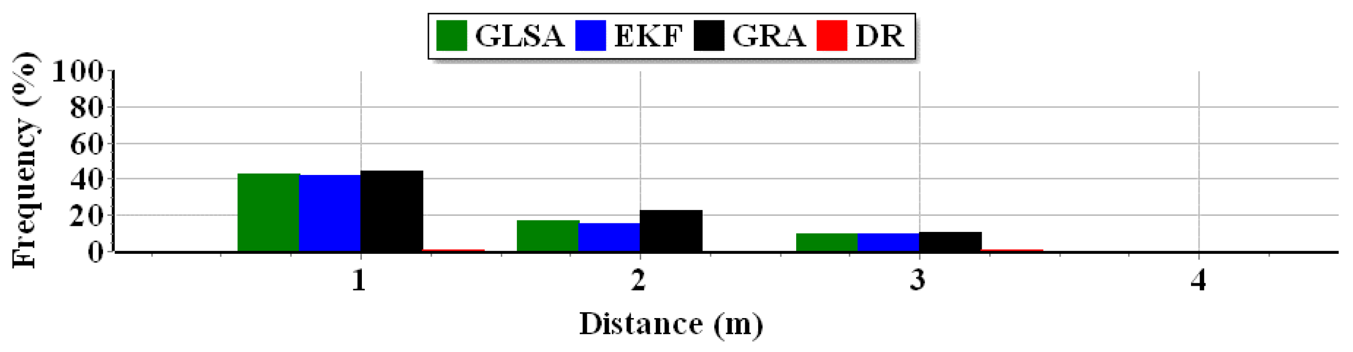
Figure 14 present the percentage of distance to the reference position from the estimated position with values falling within the ranges:
,
,
, and
.
Figure 13.
Percentage of distance to the reference position from the estimated position during a single crossing of the SV.
Figure 13.
Percentage of distance to the reference position from the estimated position during a single crossing of the SV.
Figure 14.
Percentage of distance to reference position from the estimated position during 100 SV crossings.
Figure 14.
Percentage of distance to reference position from the estimated position during 100 SV crossings.
From the bar charts in
Figure 13 and
Figure 14, it can be seen that the most significant distance percentages were obtained by: the GSLA and GRA methods in the interval
, the GRA method in the interval
, and EKF method in the interval
.
4.2. Tests Carried Out against Beacons Arranged in a Triangle
These tests simulated a single pass and 100 SV passes along a straight stretch of the road against three beacons arranged in a triangle. They resulted in two sets of analysed data, i.e., a set of five series of 300 positions and a set of five hundred series of 300 positions. Based on these,
Table 2 and
Figure 15,
Figure 16,
Figure 17,
Figure 18,
Figure 19,
Figure 20,
Figure 21,
Figure 22 and
Figure 23 were prepared for the analysis of the second group of test results.
Figure 15 shows an overview of the location of the beacons in the triangle and the estimated positions relative to them during single and 100 SV crossings.
Figure 15.
Triangle alignment of beacons and SV positions estimated relative to them during: (a) a single crossing, (b) 100 crossings.
Figure 15.
Triangle alignment of beacons and SV positions estimated relative to them during: (a) a single crossing, (b) 100 crossings.
Comparing
Figure 6 and
Figure 15 with each other, it can be seen that the estimated positions are scattered around the reference positions in similar manners. There is an increase in the scatter of positions estimated by the GLSA method, before and after the SV passes the extreme beacons (although it should be noted here that it is much smaller). The positions estimated by the EKF and GRA methods have the most considerable clustering in relation to the reference positions.
Table 2 shows the values of selected parameters of the statistical scatter of the distance to the reference position from the estimated position.
Table 2.
Statistical parameters of the scatter of the distance to the reference position from the positions estimated by the GLSA, EKF, GRA, and DR methods.
Table 2.
Statistical parameters of the scatter of the distance to the reference position from the positions estimated by the GLSA, EKF, GRA, and DR methods.
| Positioning Method | Maximum Distance to the Reference Position (m) | Arithmetic Mean of the Distance to the Reference Position (m) | Standard Deviation Distance to Reference Position (m) |
|---|
| | Single passage | 100 crossings | Single crossing | 100 crossings | Single crossing | 100 crossings |
| GLSA | 78.52 | 88.89 | 3.53 | 3.39 | 9.90 | 8.95 |
| EKF | 11.87 | 12.42 | 2.21 | 2.11 | 2.29 | 2.20 |
| GRA | 6.22 | 6.53 | 1.32 | 1.40 | 1.08 | 1.14 |
| DR | 31.48 | 30.61 | 15.22 | 16.06 | 8.32 | 8.39 |
Analysing the values of the arithmetic mean and standard deviation in
Table 2, it is possible to identify the GRA and EKF methods as clearly the best, the GLSA method as worse, and the DR method as clearly the worst. On the other hand, by comparing
Table 1 and
Table 2 with each other, it should be noted that the values of the statistical parameters relating to the GLSA and GRA methods have changed most significantly in favour (they are approximately twice as small). This is undoubtedly an effect of the non-co-linear alignment of the beacons with respect to each other (thus obtaining a better so-called ‘geometric coefficient’ calculated from the trace of the matrix
).
Figure 16 and
Figure 17 show plots of distance and arithmetic mean distance to the reference position from the estimated position during single and 100 SV crossings as a function of time.
Figure 16.
Distance to reference position from estimated position during a single SV crossing as a function of time.
Figure 16.
Distance to reference position from estimated position during a single SV crossing as a function of time.
Figure 17.
Arithmetic mean distance to the reference position from the estimated position during 100 SV crossings as a function of time.
Figure 17.
Arithmetic mean distance to the reference position from the estimated position during 100 SV crossings as a function of time.
Comparing the graphs in
Figure 7 and
Figure 8 with the graphs in
Figure 17 and
Figure 18, there is an apparent reduction in the distance to the reference position from the GLSA-estimated position from about 100 m to about 40 m in the initial and final phases of the test. The curves of the other graphs are similar to each other.
Figure 18 and
Figure 19 plot the moving mean distance to the reference position from the estimated position during a single and 100 SV crossings as a function of time.
The graphs plotted against each other in
Figure 18 and
Figure 19 clearly show that the GRA method estimates the position with the smallest moving mean distance to the reference position; this occurs almost throughout the entire test. The DR and EKF methods are only better at the beginning of the test and in a very short time frame
.
Figure 18.
Moving average distance to the reference position from the estimated position during a single SV crossing as a function of time (logarithmic scale—log base = 10).
Figure 18.
Moving average distance to the reference position from the estimated position during a single SV crossing as a function of time (logarithmic scale—log base = 10).
Figure 19.
Moving average distance to reference position from the estimated position during 100 SV crossings as a function of time (logarithmic scale—log base = 10).
Figure 19.
Moving average distance to reference position from the estimated position during 100 SV crossings as a function of time (logarithmic scale—log base = 10).
Figure 20 and
Figure 21 show plots of moving RMS to the reference position from the estimated position during a single and 100 SV crossings as a function of time.
Figure 20.
Moving RMS of the distance to the reference position from the estimated position during a single SV crossing as a function of time (logarithmic scale—log base = 10).
Figure 20.
Moving RMS of the distance to the reference position from the estimated position during a single SV crossing as a function of time (logarithmic scale—log base = 10).
Figure 21.
Moving RMS of distance to reference position from the estimated position during 100 SV crossings as a function of time (logarithmic scale—log base = 10).
Figure 21.
Moving RMS of distance to reference position from the estimated position during 100 SV crossings as a function of time (logarithmic scale—log base = 10).
Comparing
Figure 20 and
Figure 21 and
Figure 11 and
Figure 12 with each other, it is clear that the graphs relating to the DR and EKF methods have the same course and that the graphs relating to the GLSA and GRA methods are also parallel to each other. However, it is different for the GRA method. In
Figure 11 and
Figure 12, it obtains the smallest moving RMS distance values (smallest scatter around the moving average distance) over a larger time interval
.
Figure 22 and
Figure 23 present the percentage of distance to the reference position from the estimated position with values falling within the ranges:
,
,
, and
.
The bar charts in
Figure 22 and
Figure 23 show that the largest distance percentages were obtained by the GSLA and GRA methods in the interval
, the GRA method in the interval
(similar to
Figure 13 and
Figure 14), and the GRA method in the interval
.
Figure 22.
Percentage of distance to the reference point from the estimated point during a single SV crossing.
Figure 22.
Percentage of distance to the reference point from the estimated point during a single SV crossing.
Figure 23.
Arithmetic mean of the percentages of the distance to the reference point from the estimated point during 100 SV crossings.
Figure 23.
Arithmetic mean of the percentages of the distance to the reference point from the estimated point during 100 SV crossings.
4.3. Selection of the Best Method for Estimating Position Coordinates
Section 4.1 and
Section 4.2 analyse the test results. They showed that the GRA and EKF methods are interchangeably the best in terms of the accuracy of SV position coordinate estimation. On the one hand, they confirm the effectiveness of the algorithms of both methods (see
Figure 1 and
Figure 3) in suppressing the results of measurements with gross error. On the other hand, they show the interchangeability of the two methods between each other in obtaining the highest accuracy of estimated position coordinates (see
Figure 10 and
Figure 19). This mainly results from the way beacons are positioned and the location of the SV in relation to them (see
Figure 6 and
Figure 15).
Given the above, it made sense to find an objective indicator to select the most accurate positioning method depending on the SV’s location in relation to the beacons and the measurement errors of the navigation equipment.
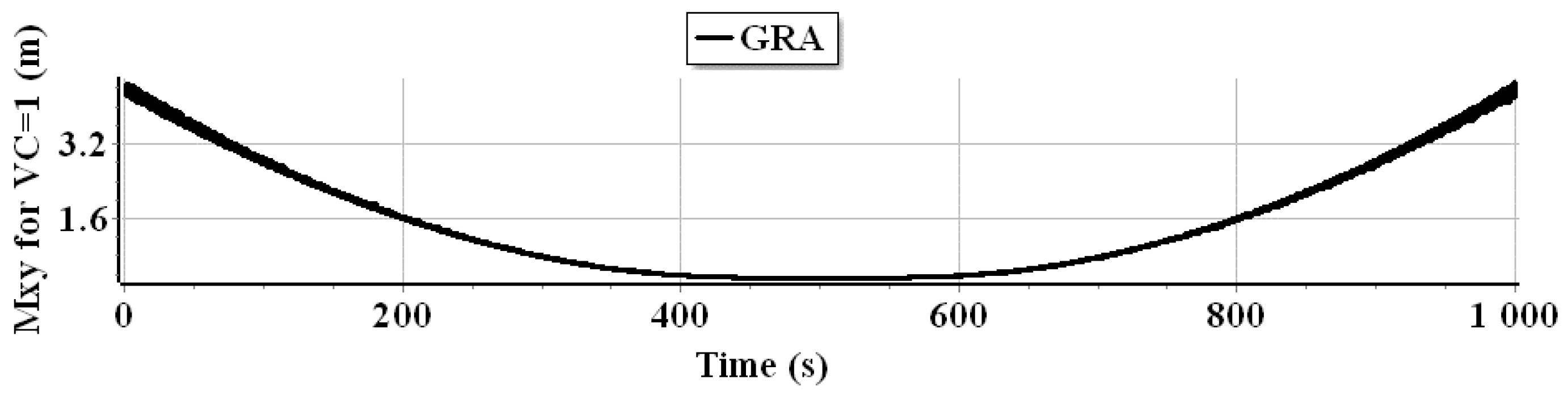
The authors of the article propose to use, for this purpose, the mean error of the
of the coordinates of the positions estimated by the GRA method. However, the value
is determined on the assumption that the mean error values of the measurements have been determined ’ideally’, i.e., the coefficient of variation (VC) has a value equal to one (see relation (
13)). Determination of the limit value
, beyond which the EKF method should be changed to GRA, should be carried out as a result of simulation tests performed for a specific navigation system.
Figure 24 and
Figure 25 show graphs of the mean error of the
of the GRA-estimated position coordinates over the course of 100 SV crossings relative to the aligned and triangular marks.
Figure 24.
Graph of mean error of GRA-estimated position coordinates over the course of 100 SV crossings, relative to aligned marks as a function of time.
Figure 24.
Graph of mean error of GRA-estimated position coordinates over the course of 100 SV crossings, relative to aligned marks as a function of time.
Figure 25.
Graph of mean error of GRA-estimated position coordinates during 100 SV crossings, relative to triangle marks as a function of time.
Figure 25.
Graph of mean error of GRA-estimated position coordinates during 100 SV crossings, relative to triangle marks as a function of time.
The graphs in
Figure 24 and
Figure 25 show that the value of the
depends not only on the iteratively determined values of the equivalent weight matrix
(see
Figure 3), but also, and mainly, on the spacing of the beacons relative to each other and the position of the SV relative to them (becoming then, so to speak, the so-called dilution of precision factor [
36]).
Nevertheless, it is essential to realise that the limit value was estimated based on simulation tests carried out under straightforward assumptions, e.g., SV only flows along a line.
Therefore, the authors of the article recommend setting a limit value depending on the number of marks and the type of measurements performed (e.g., direction only or distance only, direction and distance) and simulating the SV of a mow-the-lawn path along the area around the beacons within the achievable measurement range.
These generalised conclusions give rise to the hypothesis that the proposed methodology has great potential in supporting SV positioning in coastal and harbour waters. Along with the continuous development of measurement systems (vision, acoustic, or radar) and the high computing power, it will undoubtedly be used on a larger scale in the future. Its first implementation is planned as part of the research project entitled “Hydroacoustic positioning system for unmanned autonomous underwater vehicles” (no. DOB-SZAFIR/01/B/003/04/2021), co-financed by the Polish National Center for Research and Development (NCBR).


