A Robust Health Prognostics Technique for Failure Diagnosis and the Remaining Useful Lifetime Predictions of Bearings in Electric Motors

Featured Application

The proposed robust health prognostics technique identifies outer race bearing failures and predicts the remaining useful lifetimes of the bearings of electric motors under different working conditions. This is a major advantage for applying predictive maintenance approaches in the industry, as it helps reduce operative costs by adapting maintenance schedules to real equipment conditions.

Abstract

Remaining useful lifetime (RUL) predictions of electric motors are of vital importance in the maintenance and reduction of repair costs. Thanks to technological advances associated with Industry 4.0, physical models used for prediction and prognostics have been replaced by data-driven models that do not require specialized staff for feature selection, as the model itself learns what features are important. However, these models are usually trained and tested with the same datasets. That makes it difficult to reuse models with different datasets, so they should be retrained with data from the specific motor being analyzed. This paper presents a novel and robust health prognostics technique that predicts the remaining useful lifetime of the bearings of electric motors under different motor conditions (shaft frequency, load, type of bearing) without retraining or fine-tuning the model used. The model integrates the frequency-domain signal analysis and a stacked autoencoder (SAE) with a bidirectional long short-term memory (BiLSTM) neural network. The proposed model is trained with the IMS-bearing dataset and is then tested with IMS, FEMTO, and XJTU-SY datasets without retraining it, providing accurate results in all of them, and proving its robustness with different electric motors and work conditions.

1. Introduction

The evolution of industrial technology gives rise to a demand for more precise and effective machinery. This imposes higher reliability and safety constraints on the electric motors used in many industrial systems, such as pumps, turbines, and mills. Electric motor failure is common due to the motor’s continuous use and the conditions that many motors must withstand. The percentage breakdown of different types of motor failures is presented in various studies [1,2,3,4]. According to these studies, bearings are the most common types of motor failure, being between 40% and 50% of failures. Stator failures come in second, with approximately 30–35%. The third most common failures are rotor failures, by around 10%. All other types of failures make up the remaining percentage. Bearing failures can occur at different locations, such as in the outer race, the inner race, and the rolling elements or the bearing cage.

Maintenance has become one of the most important tasks in Industry 4.0, not only because it increases the availability of devices but also because it increases productivity. Maintenance in Industry 4.0 accounts for 15–60% of total production costs [5]. There are three different types of maintenance according to when it is performed: reactive maintenance, which is conducted when the device fails; preventive maintenance, which is carried out during planned maintenance shutdowns; and predictive maintenance, which is performed before the device is expected to fail [6]. The use of predictive maintenance means a reduction of 50–60% in maintenance costs and equipment damage, while the machine life and productivity are also increased by 50–60% and 20–30% respectively [7]. However, this type of maintenance is difficult to perform due to the need for constant monitoring of devices.

Health prognostics are essential in predictive maintenance. It focuses on predicting the remaining useful lifetime (RUL) of machinery by studying and analyzing their historical and continuing degradation trends based on data gathered by sensors [8]. Some authors refer to predictive maintenance as prescriptive maintenance when, in addition to predicting the RUL, it is also possible to identify the type of failure [9].

RUL prediction is usually carried out in four steps: feature extraction, health indicator construction, health stage division, and RUL prediction using a trained machine learning model. The first step involves selecting which features are relevant, collecting them during the operational lifetime of the machinery, and preprocessing and filtering them. The second step is the compilation of the health indicator (HI). HIs are measurements or characteristics that provide information about the condition or state of the monitored device. They can either be physical (obtained from a single feature) or virtual (obtained from a fusion of various features). The third step is performed once the curve with all values of the HI during the motor full operation cycle is obtained. It consists of dividing the HI curve into two or more stages according to the degree of degradation of the machinery. These stages can be healthy, when no degradation is observed or damaged, or when a degradation trend appears. Finally, when the HI signals a degradation state, the last step uses a machine learning model trained with run-to-failure data to predict how much life (usually cycles) of the electric motor is left until failure occurs [10,11].

The Industrial Internet of Things (IIoT) facilitates prognostics thanks to the use of sensor networks that monitor the condition of electric motors, gathering data about vibrations, temperature, and other important features [12,13]. Most of the failures in electric motors are due to bearings [1,2,3,4]. Most motor bearing failures manifest themselves differently [14] and can be detected using measurable signals, such as vibrations, stator currents, thermographs, and noise [15]. Outer race bearing failures are some of the most common causes of bearing failures since the development of variable frequency drives [16].

This paper presents a robust health prognostics technique that identifies outer race bearing failures in electric motors and predicts the RUL of the bearings of electric motors. Amplitudes of outer race bearing vibration frequencies (2X, 3X, and 4X BPFO) are used as input features and fused by means of a stacked autoencoder (SAE). Then, RUL is predicted with a bidirectional long short-term memory (BiLSTM) model. This model is trained with a dataset from the intelligent maintenance system (IMS) bearing dataset [17], tested with another dataset of IMS dataset, and validated with the FEMTO-ST Institute (FEMTO) and Xi’an Jiaotong University with Changxing Sumyoung Technology Co., Ltd. (XJTU-SY)-bearing datasets [18,19] with no retraining. This way, the proposed model is robust between different motor conditions and bearing types. The results obtained with this model are more accurate than those of similar works.

The rest of the paper is organized as follows. Previous research works are outlined in Section 2. The experimental set-up of the model is shown in Section 3. Section 4 shows the results obtained by the proposed model for training and testing and compares them with other works. Finally, Section 5 presents the concluding remarks and outlines future work.

2. Background

Much research effort in the field of RUL prediction has been made in the last decade. Although there is no standardized procedure, most of the related works divide RUL prediction into four steps: feature extraction, health indicator construction, health stage division, and RUL prediction.

The first step consists of gathering data from the monitored machinery. IIoT has facilitated this task using wireless sensor networks composed of different types of sensors. Vibrations [20,21], acoustic emissions [22,23], temperatures [24], and current measurements [25,26] are among the most commonly used data in the RUL prediction of electric motors. However, gathering run-to-failure data from running machinery for training the prognostic model is unfeasible because a run-to-failure breakdown may cause the complete breakdown of the machinery with unpredictable consequences [8]. In order to build prognostic models, there are public datasets that contain data acquired from accelerated degradation tests. There are several publicly available run-to-failure datasets of electric motors. The most commonly used in health prognostics of electric motors are the FEMTO-bearing dataset and the IMS-bearing dataset [17,18].

In the second step, health indicators (HIs) are constructed in order to predict the health status of the monitored machinery. They can be of two types depending on the technique used to construct them: physical HIs (PHIs) and virtual HIs (VHIs) [8]. PHIs are health indicators that are based on the physical properties of the monitored machinery, such as vibration or temperature. They can also be determined by a single feature extracted from monitored signals using signal processing techniques, such as wavelets [24] and fast Fourier transforms (FFTs) [26], or statistical methods, such as RMS, Kurtosis, and skewness [20,22,26]. VHIs are health indicators derived from data collected from the monitored machinery and are related to physical properties but are not necessarily measurements of those properties. They can be used to supplement or replace PHIs, and are more convenient and cost-effective to obtain in some cases. Techniques commonly used to fuse features and reduce their dimensionality are the principal component analysis (PCA) [27,28], stacked autoencoders (SAEs) [29], Mahalanobis distance [30], and Kalman filters [21,25], as well as artificial intelligence techniques, such as fuzzy networks [31], convolutional neural networks (CNNs) [32], and recurrent neural networks (RNNs) [33,34,35].

The third step comprises the HI stage division. Depending on the trend of the HI curve, this can be split into multiple stages. Each of these stages provides boundaries or points for predicting RUL [36]. Many studies divide the HI curve into two stages, which are the normal operation condition and failure condition [37]. However, other works, in which the slope of the HI curve is less pronounced, divide the HI curve into four stages: normal, mild degradation, moderate degradation, and near-to-failure [38].

The last step of health prognostics is the actual RUL prediction. There are different types of RUL prediction models depending on the type of data, methodology, algorithm, or even previous knowledge about the machinery to be analyzed [39]. Physics-based approaches use physical laws and principles to model the behavior of the monitored machinery over time. They provide the highest accuracy and precision, albeit with the disadvantage that they require expert knowledge to perform an in-depth analysis of the training dataset. These models have to be developed from scratch, thus limiting reusability with other similar datasets [40,41]. Another alternative is the data-driven approach, which uses statistical methods, such as random coefficient models [42,43], Wiener process models [44,45], or proportional hazards models [46], as well as those that use machine learning models, such as artificial neural networks (ANNs) [47,48], gated recurrent units (GRUs) [49,50], long short-term memory (LSTM) [51,52,53], or CNNs [32]. These approaches can be effective without requiring expert knowledge in cases where there are large amounts of data available. However, they do not provide a detailed understanding of the underlying physical processes. There are also hybrid approaches that combine elements of both physics-based and data-driven approaches, using physical models to provide a detailed understanding of the monitored machinery, but also using data-driven techniques to simplify the model development. These approaches are effective in cases where there are limited amounts of data but a detailed understanding of the monitored machinery is required [54,55]. In general, physics-based approaches offer a deeper understanding of physical processes, but they are more complex for model development and validation. On the other hand, data-driven approaches are simpler and more effective with large amounts of data, but they do not offer insight into the underlying physical processes. Hybrid approaches offer a compromise between accuracy and simplicity.

Most of the works using data-driven approaches for RUL prediction use the same bearing dataset for both training and testing. Liu et al. [56] developed a health prognostics technique that uses the Hilbert–Huang transform to extract failure signals based on Spearman’s coefficient, and fuses them into a single feature by means of normalized partial derivative weights. The HI curve is then estimated using a recursive likelihood estimation model (RMLE). In the work presented by Yoo and Baek [57], images obtained after applying the wavelet transform are used as input features. A 2D convolutional neural network is used to combine them and a Gaussian process regression (GPR) model is then used to predict the RUL. The Laplacian score (LS) with the LSTM network is used in the work presented by Saufi and Hassan [58], using LS to select the best time-domain features and LSTM to predict RUL. Guo et al. [33] used six time-frequency domain features that were fused using RNNs into a single one. RUL prediction was carried out by using a double exponential model. In the work presented by Xu et al. [59], convolutional autoencoder (CAE) networks were used to extract features, and a subsequent status degradation model was used to predict the RUL. The robustness of these works was not tested, as they used the FEMTO dataset for both training and testing. Similarly, the same issue is present in the work by Kong and Li [60], where time-domain features were extracted manually and then used to predict the RUL by means of a stacked bidirectional LSTM neural network using the XJTU-SY dataset.

To cover this gap, this work proposes a health prognostics technique that identifies outer race bearing failures and predicts the RUL of electric motor bearings. The proposed model identifies an unambiguous signature of the outer race bearing failures regardless of the motor-working conditions, which provides it with the necessary robustness to correctly predict the RUL, obtaining accurate results on other datasets where the motor used is different or works under different conditions than the one used for training, without the need for retraining the model. This is a significant contribution as it allows the model to be applied to a wider range of electric motors working at different conditions and potentially improves maintenance schedules for electric motors. Additionally, the ability to predict RUL and identify bearing failures can help prevent unexpected breakdowns and improve the overall reliability and efficiency of the electric motors.

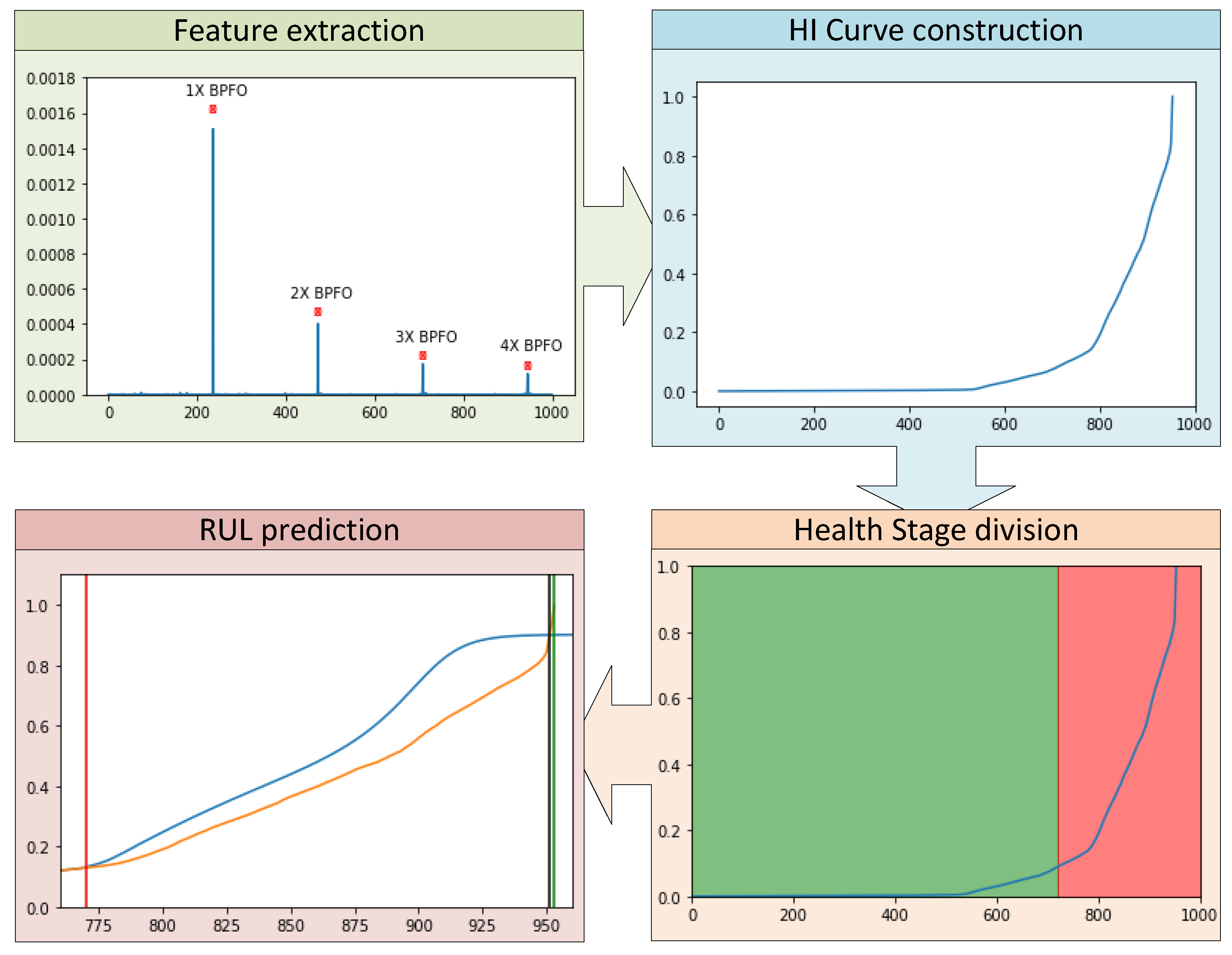
3. Proposed Solution

A robust health prognostics technique that identifies outer race bearing failure and predicts the RUL of different electric motor bearings without retraining has been developed. The following subsections present the developed health prognostics technique, dividing it into the four main steps shown in Figure 1: feature extraction, HI curve construction, health stage division, and RUL prediction.

3.1. Feature Extraction

Electric motors may suffer from many different types of failures, most of which, including those related to bearings, are manifested in the vibration signal of the motor. Vibration can be measured using displacement, velocity, and acceleration units. Since bearing failures tend to manifest themselves at high frequencies, acceleration is preferred, as higher frequency vibrations have less displacement and velocity for the same amount of power.

Frequency-domain analysis techniques are more precise in identifying bearing failures. However, using the conventional FFT technique to extract frequency features from the raw data is inadequate, since the real vibration signals are non-stationary and the useful part of the bearing vibration signal can be hidden or covered by noise and disturbances. The Hilbert–Huang transform (HHT) [61] is widely used to analyze non-stationary signals arising out of defective rolling element bearings. HHT uses an empirical mode decomposition (EMD) process to decompose the raw signal into various intrinsic functions (IMFs) and a residue. Then, these IMFs are transformed using the Hilbert transform.

IMFs contain frequencies in decreasing order, with the first IMF showing the highest frequencies contained in the denoised vibration signal [62]. Thus, the envelope of the first IMF of the decomposed vibration signal using HHT is transformed into the frequency domain using the FFT, so the amplitudes of the most interesting frequency bins are extracted.

After empirically studying different sets of input features, the amplitudes of the bins corresponding to frequencies of 2X, 3X, and 4X $BPFO$ provide the best results. $BPFO$ is obtained with Equation (1), where N is the number of balls of the bearings, F is the shaft frequency ($Hz$), B is the ball diameter (mm), P is the pitch diameter (mm), and $\theta$ is the contact angle.

$$BPFO=\frac{N}{2}\times F\times \left(1-\frac{B}{P}\times cos\theta \right)$$

(1)

Errors in data gathering and the bearings not rotating smoothly can be issues when computing the FFT, causing the amplitudes of the bins to appear slightly off. To avoid this and to ensure the best performance, the amplitudes of the desired frequencies are obtained from Equation (2), where the amplitude of the bin ($A_n$) is obtained as the maximum of the raw amplitudes of bins $a_{n-4}$ to $a_{n+4}$.

$$A_n=max\{a_{n-4},\cdots ,a_{n+4}\}$$

(2)

3.2. HI Curve Construction

The second step is to create a curve with the history of values of the HI. It is necessary to normalize all extracted features before constructing the HI. The amplitudes of the bins are normalized using min–max normalization, as shown in Equation (3). This normalizes data between 0 and 1 in order to represent the degradation of the electric motor, where 0 means no failure and 1 full degradation. For testing, when the top end of the scale of the time-domain feature is not yet known, the maximum value used to normalize is the maximum value for each input feature of the set used for training. This is done in order to determine a common full scale for normalization.

$$x_{norm}=\frac{x-min\left(x\right)}{max\left(x\right)-min\left(x\right)}$$

(3)

Once the features are normalized, they are fused and denoised using a stacked autoencoder (SAE). Autoencoders (AEs) are unsupervised machine learning algorithms based on encoders, which convert the high-dimensional input into a low-dimensional output, and a decoder, which reconstructs the input data from the low-dimensional output generated by the encoder. An SAE is an AE with a deeper neural network and symmetric dimensions of the encoding and decoding sets. The ability of SAEs to denoise signals has been widely used in many domains, such as image processing [63] or fault detection [64] to name a few, as it is able to learn a compressed representation that contains only the essential information of each feature.

The SAE network is built using TensorFlow in the Keras framework with 3–2–1–2–3 structure, where 3 corresponds to the 3 normalized input features, 2 is the number of nodes at the first and third hidden layers, and 1 is the dimension of the feature obtained from the first hidden layer, which is the health indicator. The hyperparameters used by the SAE network are included in

Table 1. SAE hyperparameters.

SAE Structure	3–2–1–2–3
Activation function	ReLu
Optimizer	Adam
Learning rate	0.001
Epochs	20

. A schematic diagram of the SAE model structure is shown in Figure 2. The three normalized and one-dimensional input features correspond to the normalized values of the amplitudes of bins 2X, 3X, and 4X BPFO gathered during the lifetime of the electric motor. The encoder fuses these input features into a low-dimensional feature, which is called HI value. The purpose of the decoder is to reconstruct the original input from the encoded representation (HI value) produced by the encoder. It takes the encoded representation as input and generates an output that should be as similar as possible to the original input data. This reconstruction process allows the SAE to learn a compact and informative representation of the input data, containing only the most important information.

An exponentially weighted moving average function (EWMA) is then used to smooth the obtained HI. EWMA functions give higher weights to the most recent values. The Pandas ewm function is used to smooth the obtained HI, with a center of mass of 5. The smoothed HI is finally normalized using min–max normalization.

3.3. Health Stage Division

The HI curve is divided into two stages based on its trend. The first stage corresponds to the correct operation of the electric motor, where a stable trend can be seen. The second stage starts with the appearance of failures or anomalies in the operation of the equipment, where an increasing trend of the curve is seen. An example of how the HI curve is divided into healthy (green area) and damaged (red area) stages is shown in Figure 3.

The threshold separating the two areas is determined as the first point where the difference between the HI predicted in 75 cycles and the HI at that time is greater than 0.02. It is in the red area when the RUL should be predicted.

3.4. RUL Prediction

RUL prediction is performed by forecasting the HI curve. Recurrent neural networks (RNNs) are very effective at sequence modeling. In this work, a bidirectional long short-term memory (BiLSTM) model was developed to predict RUL. BiLSTM is a form of artificial RNN, which is typically used to extract the long-term dependencies of input sample data. It is composed of two LSTM layers, one used for forward propagation and the other used for backward propagation, enabling the flow in both directions [25].

LSTM cells have three gates, which manage the flow of information throughout the network: the input, forget, and output gates. The input gate is open when the inward information flow is activated and closed when it is deactivated. The output gate works similarly; outward information flow is disabled if the gate is closed. The forget gate decides which information is to be retained and which can be forgotten. A BiLSTM connects two LSTM layers to the output layer, making the model performance better than with LSTM. The output $\overrightarrow{h}$ from the forward LSTM layer is obtained as with a regular LSTM, while the output $\overleftarrow{h}$ obtained from the backward layer is computed using the reversed inputs from time $t-1$ to $t-n$. Both outputs are then combined using the sigmoid function into an output vector $y_t$ [65]. The structure of a BiLSTM layer is shown in Figure 4.

The network structure and hyperparameters of the BiLSTM network are listed in

Table 2. BiLSTM hyperparameters.

BiLSTM Structure	1-5-60-5-1
Activation function	ReLu
Optimizer	Adam
Learning rate	0.001
Epochs	1000

. The 60-node layer corresponds to the BiLSTM layer, which is composed of 2 LSTM layers of 30 nodes each. To perform RUL prediction, the HI curve is used as the input feature. The sequence feature and the sliding step sizes used are 10 and 1, respectively. This means that if the input sequence feature is $[X_1,X_2,X_3,\dots ,X_{10}]$, the prediction function can be expressed as $F\left([X_1,X_2,X_3,\dots ,X_{10}]\right)=Y_{11}$. This process can be used to forecast the HI curve by computing $F\left([X_2,X_3,\dots ,X_{10},Y_{11}]\right)=Y_{12}$, $F\left([X_3,X_4,\dots ,X_{10},Y_{11},Y_{12}]\right)=Y_{13}$, and so on, obtaining the output sequence $[X_1,X_2,X_3,\dots ,X_{10},Y_{11},Y_{12},\dots ,Y_z]$ where z corresponds to the number of predictions.

Once the HI curve is predicted, the point n that determines the moment of failure is selected. This corresponds to the first predicted value that satisfies the following condition: $|Y_n-Y_{n+100}|\le 0.001$. This value is selected empirically once the training phase is up and does not change after training, proving its robustness while predicting RUL with different datasets. In order to compare the results obtained by the proposed solution with other works, the error in RUL prediction is used. The error is computed following Equation (4), where $R_A$ corresponds to the actual RUL, $R_P$ corresponds to the predicted RUL, and $P_t$ corresponds to the time when the prediction is made. Negative errors mean that the predicted RUL is longer than the actual RUL (underestimate), while positive errors mean that the predicted RUL is shorter than the actual RUL (overestimate). Overestimates are preferable because they lead to early predictions, allowing maintenance work or part replacements to be planned before motor failure occurs.

$$error=\frac{(R_A-P_t)-(R_P-P_t)}{R_A-P_t}\times 100$$

(4)

4. Results

This section is divided into three subsections. Achievements of the model in the training and test phases are shown in Section 4.1 and Section 4.2, respectively. An example of how the model discriminates outer race failures from other types of bearing failures is shown in Section 4.3. The datasets used in training and testing are shown in

Table 3. Dataset information.

Name	Samples	Total Time	Bearing Type	Shaft Frequency	Load	BPFO	Used in
IMS dataset no. 2	984	6 d 20 h	Rexnord ZA-2115	33.33 Hz	26.69 kN	236 Hz	Training
IMS dataset no. 3	4448	31 d 10 h					Testing
FEMTO Bearing1_3	2376	6 h 36 m	NSK 6804-DD	30 Hz	4 kN	168.34 Hz	Testing
FEMTO Bearing1_4	1429	3 h 58 m
FEMTO Bearing1_7	2260	6 h 16 m
XJTU-SY Bearing2_5	339	5 h 39 m	LDK UER204	37.5 Hz	11 kN	115.61 Hz	Testing
XJTU-SY Bearing3_1	2538	42 h 18 m		40 Hz	10 kN	123.32 Hz

.

4.1. Model Training

In order to train the model, IMS dataset no. 2 was used. It has a total of 984 run-to-failure samples, corresponding to a motor operation of 6 days and 20 h. Accelerations were collected at a frequency of 20 kHz and outer race bearing failure was detected at the end of the test. This motor works at a frequency of 33.33 Hz and has a load of 26.69 kN. The bearing used was Rexnord ZA-2115.

Firstly, HHT was used to preprocess the vibration signal. Then FFT was computed on the envelope of the first IMF for each sample to extract the amplitudes of the bins corresponding to 2X, 3X, and 4X BPFO. The motor used in the IMS dataset has a BPFO of 236 Hz, so the frequencies corresponding to 2X, 3X, and 4X are 472, 708, and 944 Hz, respectively. Before fusing these features into the HI curve, it is necessary to normalize them separately using min–max normalization. After that, the fusing of the features is carried out using the SAE network. Figure 5 shows the normalized features and the HI curve obtained.

The BiLSTM model was trained on 70% of the randomly selected data set. After training, the rest of the dataset was used to forecast the HI curve in order to compare it with the actual HI curve. RUL prediction results with the training dataset are shown in Figure 6. The vertical dashed red line corresponds to the instant at which the prediction is made. In turn, the green line corresponds to the actual RUL, while the dashed black line corresponds to the predicted RUL. The error obtained with the developed model in IMS dataset no. 2 is 1.0869%.

4.2. Model Testing

The trained model was tested on other datasets with outer race bearing failures in order to validate its correct performance. In total, three different datasets were used for testing.

Firstly, it was tested with IMS dataset no. 3, which has 4448 samples corresponding to 31 days and 10 h of motor operation. This motor works under the same conditions as the one used in IMS dataset no. 2.

Three different datasets (Bearing1_3, Bearing1_4, and Bearing 1_7) from the FEMTO dataset were also used. Bearing1_3 has 2376 samples corresponding to 6 h and 36 min of motor operation; Bearing1_4 has 1429 samples corresponding to 3 h and 58 min of motor operation and Bearing1_7 has 2260 samples corresponding to 6 h and 16 min of motor operation. In all of them, the motor works at 30 Hz and 4 kN of load using an NSK6804DD bearing, which has a BPFO of 168.34 Hz.

Finally, two datasets (Bearing2_5 and Bearing3_1) from the XJTU-SY dataset were used, each with different motor operating conditions. The first one has a total of 339 samples, corresponding to 5 h and 39 min of motor operation working at 37.5 Hz with a load of 11 kN. The other one has a total of 2538 samples, corresponding to 42 h and 18 min of motor operation at 40 Hz with a load of 10 kN. The bearings used in both tests are LDK UER204, which has a BPFO of 115.61 Hz for the first dataset and a BPFO of 123.32 Hz for the second dataset.

RUL predictions are shown in Figure 7 for each dataset. The errors in predicting RUL with IMS, FEMTO, and XJTU-SY datasets are also shown in

Table 4. RUL results in comparison with other works.

				Prediction Error (%)
Testing Dataset	${\mathit{P}}_{\mathit{t}}$	${\mathit{R}}_{\mathit{A}}$	${\mathit{R}}_{\mathit{P}}$	Proposed Model	[33]	[56]	[57]	[58]	[59]	[60]
IMS dataset no. 3	6174	6315	6314	0.71	-	-	-	-	-	-
FEMTO Bearing 1_3	2200	2376	2374	0.91	43.28	2.58	1.05	−0.69	−2.62	-
FEMTO Bearing 1_4	1247	1428	1427	1.75	67.55	−9.14	20.35	3.10	17.40	-
FEMTO Bearing 1_7	2030	2260	2254	2.08	17.83	−0.70	29.19	7.00	1.06	-
XJTU-SY Bearing 2_5	265	338	338	1.52	-	-	-	-	-	8.95
XJTU-SY Bearing 3_1	2433	2527	2525	1.06	-	-	-	-	-	10.42

. While predicting RUL with IMS dataset no. 3, the error is 0.71%. For FEMTO and XJTU-SY datasets, the errors are also compared with the errors reported in similar works that tested their model with those datasets. As can be seen, in the FEMTO Bearing1_7 dataset, the error is 2.08%, second only to that in the work by Xu et al. [59]. In the FEMTO Bearing1_3 and FEMTO Bearing1_4 datasets, the errors are significantly lower than those in the rest of the works. The errors with the XJTU-SY dataset are always below 1.52%, improving the results obtained in the work presented by Kong and Li [60]. All of these errors are positive, which means that the predicted RUL is overestimated. Overestimations are preferable because they lead to early predictions, allowing maintenance work or part replacements to be planned before motor failure occurs.

4.3. Model Discrimination

One of the advantages of this model is that it does not predict a general RUL. It predicts RUL based on outer race bearing failures. Thus, the model is suitable for prescriptive maintenance, because apart from predicting the time before failure, it provides information about a specific kind of failure in the motor.

The model was tested with IMS dataset no. 1, which presents inner race rather than outer race failures. Figure 8 shows the RUL prediction results obtained by the proposed model (Figure 8a) and by the work presented by Saufi and Hassan [58] (Figure 8b, extracted from their paper). As seen in Figure 8a, the HI curve predicted by the proposed model stays near 0, meaning that there will be no outer race failure in the future. However, in the work presented by Saufi and Hassan [58], the RUL prediction shows that in cycle 2184 there will be an unspecified failure.

5. Conclusions and Future Work

A novel robust health prognostics technique that identifies outer race bearing failures and predicts the remaining useful lifetime of the bearings of electric motors was designed, implemented, trained, and tested. HHT for data preprocessing, frequency-domain analysis using FFT for feature extraction, stacked autoencoders (SAEs) for feature denoising and feature fusion, and bidirectional long short-term memory (BiLSTM) for RUL prediction were used to build the prediction model.

The robustness of the proposed model was demonstrated while predicting the RUL of bearings with different motors and motor operating conditions (shaft frequency, load, type of bearing), without retraining or fine-tuning the model. The most popular datasets for RUL prediction in electric motors have been used. IMS dataset no. 2 was used for training while IMS dataset no. 3, FEMTO, and XJTU-SY bearing datasets were used for testing the developed model, validating it with a total of four different motor operating conditions. The results obtained with the FEMTO and XJTU-SY bearing datasets are more accurate than those of previous works trained and tested with the same dataset, without demonstrating the robustness of their models to changes in motor or motor conditions. Its robustness, high accuracy, and fast prediction make the proposed health prognostics technique suitable for predicting RUL in electric motors working under different conditions.

Future work will be geared toward developing new health prognostic techniques that predict RUL and identify other types of bearing failures, such as inner race or ball-bearing failures. The ultimate objective was geared toward prescriptive maintenance, combining all of these health prognostics techniques in order to predict RUL, identify different kinds of failures, and provide information about the extent to which they contribute to the bearing degradation.

References

1. Hashemian, H. Wireless sensors for predictive maintenance of rotating equipment in research reactors. Ann. Nucl. Energy 2011, 38, 665–680. [Google Scholar] [CrossRef]
2. Bazurto, A.J.; Quispe, E.C.; Mendoza, R.C. Causes and failures classification of industrial electric motor. In Proceedings of the 2016 IEEE ANDESCON, Arequipa, Peru, 19–21 October 2016; pp. 1–4. [Google Scholar]
3. Merizalde, Y.; Hernández-Callejo, L.; Duque-Perez, O. State of the art and trends in the monitoring, detection and diagnosis of failures in electric induction motors. Energies 2017, 10, 1056. [Google Scholar] [CrossRef]
4. Lu, B.; Durocher, D.B.; Stemper, P. Predictive maintenance techniques. IEEE Ind. Appl. Mag. 2009, 15, 52–60. [Google Scholar] [CrossRef]
5. Zonta, T.; Da Costa, C.A.; da Rosa Righi, R.; de Lima, M.J.; da Trindade, E.S.; Li, G.P. Predictive maintenance in the Industry 4.0: A systematic literature review. Comput. Ind. Eng. 2020, 150, 106889. [Google Scholar] [CrossRef]
6. Li, Y.; He, Y.; Liao, R.; Zheng, X.; Dai, W. Integrated predictive maintenance approach for multistate manufacturing system considering geometric and non-geometric defects of products. Reliab. Eng. Syst. Saf. 2022, 228, 108793. [Google Scholar] [CrossRef]
7. Gholaminejad, A.; Bidgoli, F.S.; Poshtan, J.; Poshtan, M. A novel kurtogram-based health index for induction motor fault diagnosis. In Proceedings of the 2019 International Aegean Conference on Electrical Machines and Power Electronics (ACEMP) & 2019 International Conference on Optimization of Electrical and Electronic Equipment (OPTIM), Istanbul, Turkey, 27–29 August 2019; pp. 85–92. [Google Scholar]
8. Lei, Y.; Li, N.; Guo, L.; Li, N.; Yan, T.; Lin, J. Machinery health prognostics: A systematic review from data acquisition to RUL prediction. Mech. Syst. Signal Process. 2018, 104, 799–834. [Google Scholar] [CrossRef]
9. Ansari, F.; Glawar, R.; Nemeth, T. PriMa: A prescriptive maintenance model for cyber-physical production systems. Int. J. Comput. Integr. Manuf. 2019, 32, 482–503. [Google Scholar] [CrossRef]
10. Kordestani, M.; Saif, M.; Orchard, M.E.; Razavi-Far, R.; Khorasani, K. Failure prognosis and applications—A survey of recent literature. IEEE Trans. Reliab. 2019, 70, 728–748. [Google Scholar] [CrossRef]
11. Baur, M.; Albertelli, P.; Monno, M. A review of prognostics and health management of machine tools. Int. J. Adv. Manuf. Technol. 2020, 107, 2843–2863. [Google Scholar] [CrossRef]
12. Magadán, L.; Suárez, F.; Granda, J.; García, D. Low-Cost Industrial IoT System for Wireless Monitoring of Electric Motors Condition. Mob. Netw. Appl. 2022, 1–10. [Google Scholar] [CrossRef]
13. Aruquipa, G.; Diaz, F. An IoT architecture based on the control of Bio Inspired manufacturing system for the detection of anomalies with vibration sensors. Procedia Comput. Sci. 2022, 200, 438–450. [Google Scholar] [CrossRef]
14. Liu, Y.; Chen, Z.; Tang, L.; Zhai, W. Skidding dynamic performance of rolling bearing with cage flexibility under accelerating conditions. Mech. Syst. Signal Process. 2021, 150, 107257. [Google Scholar] [CrossRef]
15. Zhang, S.; Zhang, S.; Wang, B.; Habetler, T.G. Deep learning algorithms for bearing fault diagnostics—A comprehensive review. IEEE Access 2020, 8, 29857–29881. [Google Scholar] [CrossRef]
16. Zamudio-Ramirez, I.; Osornio-Rios, R.A.; Antonino-Daviu, J.A.; Cureño-Osornio, J.; Saucedo-Dorantes, J.J. Gradual Wear Diagnosis of Outer-Race Rolling Bearing Faults through Artificial Intelligence Methods and Stray Flux Signals. Electronics 2021, 10, 1486. [Google Scholar] [CrossRef]
17. Qiu, H.; Lee, J.; Lin, J.; Yu, G. Wavelet filter-based weak signature detection method and its application on rolling element bearing prognostics. J. Sound Vib. 2006, 289, 1066–1090. [Google Scholar] [CrossRef]
18. Nectoux, P.; Gouriveau, R.; Medjaher, K.; Ramasso, E.; Chebel-Morello, B.; Zerhouni, N.; Varnier, C. PRONOSTIA: An experimental platform for bearings accelerated degradation tests. In Proceedings of the IEEE International Conference on Prognostics and Health Management, Denver, CO, USA, 18–22 June 2012; pp. 1–8. [Google Scholar]
19. Wang, B.; Lei, Y.; Li, N.; Li, N. A hybrid prognostics approach for estimating remaining useful life of rolling element bearings. IEEE Trans. Reliab. 2018, 69, 401–412. [Google Scholar] [CrossRef]
20. Lee, C.Y.; Huang, T.S.; Liu, M.K.; Lan, C.Y. Data science for vibration heteroscedasticity and predictive maintenance of rotary bearings. Energies 2019, 12, 801. [Google Scholar] [CrossRef]
21. Lee, M.S.; Shifat, T.A.; Hur, J.W. Kalman Filter Assisted Deep Feature Learning for RUL Prediction of Hydraulic Gear Pump. IEEE Sens. J. 2022, 22, 11088–11097. [Google Scholar] [CrossRef]
22. Motahari-Nezhad, M.; Jafari, S.M. Bearing remaining useful life prediction under starved lubricating condition using time domain acoustic emission signal processing. Expert Syst. Appl. 2021, 168, 114391. [Google Scholar] [CrossRef]
23. AlShorman, O.; Alkahatni, F.; Masadeh, M.; Irfan, M.; Glowacz, A.; Althobiani, F.; Kozik, J.; Glowacz, W. Sounds and acoustic emission-based early fault diagnosis of induction motor: A review study. Adv. Mech. Eng. 2021, 13, 1687814021996915. [Google Scholar] [CrossRef]
24. Belmiloud, D.; Benkedjouh, T.; Lachi, M.; Laggoun, A.; Dron, J. Deep convolutional neural networks for Bearings failure predictionand temperature correlation. J. Vibroeng. 2018, 20, 2878–2891. [Google Scholar] [CrossRef]
25. Shifat, T.A.; Yasmin, R.; Hur, J.W. A Data Driven RUL Estimation Framework of Electric Motor Using Deep Electrical Feature Learning from Current Harmonics and Apparent Power. Energies 2021, 14, 3156. [Google Scholar] [CrossRef]
26. Dameshghi, A.; Refan, M.H. Combination of condition monitoring and prognosis systems based on current measurement and PSO-LS-SVM method for wind turbine DFIGs with rotor electrical asymmetry. Energy Syst. 2021, 12, 203–232. [Google Scholar] [CrossRef]
27. Zheng, L.; He, Y.; Chen, X.; Pu, X. Optimization of Dilated Convolution Networks with Application in Remaining Useful Life Prediction of Induction Motors. Measurement 2022, 200, 111588. [Google Scholar] [CrossRef]
28. Cao, R.; Yunusa-Kaltungo, A. An Automated Data Fusion-Based Gear Faults Classification Framework in Rotating Machines. Sensors 2021, 21, 2957. [Google Scholar] [CrossRef]
29. Han, T.; Pang, J.; Tan, A.C. Remaining useful life prediction of bearing based on stacked autoencoder and recurrent neural network. J. Manuf. Syst. 2021, 61, 576–591. [Google Scholar] [CrossRef]
30. Lin, M.; Shan, M.; Zhou, J.; Pan, Y. A Data-Driven Fault Diagnosis Method Using Modified Health Index and Deep Neural Networks of a Rolling Bearing. J. Comput. Inf. Sci. Eng. 2022, 22, 021005. [Google Scholar] [CrossRef]
31. Shen, Z.; He, Z.; Chen, X.; Sun, C.; Liu, Z. A monotonic degradation assessment index of rolling bearings using fuzzy support vector data description and running time. Sensors 2012, 12, 10109–10135. [Google Scholar] [CrossRef]
32. Xu, X.; Li, X.; Ming, W.; Chen, M. A novel multi-scale CNN and attention mechanism method with multi-sensor signal for remaining useful life prediction. Comput. Ind. Eng. 2022, 169, 108204. [Google Scholar] [CrossRef]
33. Guo, L.; Li, N.; Jia, F.; Lei, Y.; Lin, J. A recurrent neural network based health indicator for remaining useful life prediction of bearings. Neurocomputing 2017, 240, 98–109. [Google Scholar] [CrossRef]
34. Senanayaka, J.S.L.; Van Khang, H.; Robbersmyr, K.G. Autoencoders and recurrent neural networks based algorithm for prognosis of bearing life. In Proceedings of the 2018 21st International Conference on Electrical Machines and Systems (ICEMS), Jeju, Republic of Korea, 7–10 October 2018; pp. 537–542. [Google Scholar]
35. Wang, G.; Li, H.; Zhang, F.; Wu, Z. Feature Fusion based Ensemble Method for remaining useful life prediction of machinery. Appl. Soft Comput. 2022, 129, 109604. [Google Scholar] [CrossRef]
36. Chen, C.; Lu, N.; Jiang, B.; Xing, Y.; Zhu, Z.H. Prediction interval estimation of aeroengine remaining useful life based on bidirectional long short-term memory network. IEEE Trans. Instrum. Meas. 2021, 70, 1–13. [Google Scholar] [CrossRef]
37. Calabrese, F.; Regattieri, A.; Bortolini, M.; Gamberi, M.; Pilati, F. Predictive maintenance: A novel framework for a data-driven, semi-supervised, and partially online prognostic health management application in industries. Appl. Sci. 2021, 11, 3380. [Google Scholar] [CrossRef]
38. Zhou, H.; Huang, J.; Lu, F. Reduced kernel recursive least squares algorithm for aero-engine degradation prediction. Mech. Syst. Signal Process. 2017, 95, 446–467. [Google Scholar] [CrossRef]
39. Wang, Y.; Zhao, Y.; Addepalli, S. Remaining useful life prediction using deep learning approaches: A review. Procedia Manuf. 2020, 49, 81–88. [Google Scholar] [CrossRef]
40. Kumar, S.; Dutta, S.K.; Ghoshal, S.K.; Das, J. Model-Based Adaptive Prognosis of a Hydraulic System. In Recent Advances in Mechanical Engineering; Springer: Singapore, 2020; pp. 375–391. [Google Scholar]
41. Qian, Y.; Yan, R.; Gao, R.X. A multi-time scale approach to remaining useful life prediction in rolling bearing. Mech. Syst. Signal Process. 2017, 83, 549–567. [Google Scholar] [CrossRef]
42. Tse, P.W.; Wang, D. Enhancing the abilities in assessing slurry pumps’ performance degradation and estimating their remaining useful lives by using captured vibration signals. J. Vib. Control 2017, 23, 1925–1937. [Google Scholar] [CrossRef]
43. Jin, X.; Sun, Y.; Que, Z.; Wang, Y.; Chow, T.W. Anomaly detection and fault prognosis for bearings. IEEE Trans. Instrum. Meas. 2016, 65, 2046–2054. [Google Scholar] [CrossRef]
44. Huang, Z.; Xu, Z.; Ke, X.; Wang, W.; Sun, Y. Remaining useful life prediction for an adaptive skew-Wiener process model. Mech. Syst. Signal Process. 2017, 87, 294–306. [Google Scholar] [CrossRef]
45. Li, N.; Lei, Y.; Lin, J.; Ding, S.X. An improved exponential model for predicting remaining useful life of rolling element bearings. IEEE Trans. Ind. Electron. 2015, 62, 7762–7773. [Google Scholar] [CrossRef]
46. Wang, L.; Zhang, L.; Wang, X.z. Reliability estimation and remaining useful lifetime prediction for bearing based on proportional hazard model. J. Cent. South Univ. 2015, 22, 4625–4633. [Google Scholar] [CrossRef]
47. Scalabrini Sampaio, G.; Vallim Filho, A.R.d.A.; Santos da Silva, L.; Augusto da Silva, L. Prediction of motor failure time using an artificial neural network. Sensors 2019, 19, 4342. [Google Scholar] [CrossRef] [PubMed]
48. Shifat, T.A.; Hur, J.W. ANN assisted multi sensor information fusion for BLDC motor fault diagnosis. IEEE Access 2021, 9, 9429–9441. [Google Scholar] [CrossRef]
49. Chen, J.; Jing, H.; Chang, Y.; Liu, Q. Gated recurrent unit based recurrent neural network for remaining useful life prediction of nonlinear deterioration process. Reliab. Eng. Syst. Saf. 2019, 185, 372–382. [Google Scholar] [CrossRef]
50. Ding, N.; Li, H.; Xin, Q.; Wu, B.; Jiang, D. Multi-source domain generalization for degradation monitoring of journal bearings under unseen conditions. Reliab. Eng. Syst. Saf. 2022, 230, 108966. [Google Scholar] [CrossRef]
51. Lu, B.L.; Liu, Z.H.; Wei, H.L.; Chen, L.; Zhang, H.; Li, X.H. A deep adversarial learning prognostics model for remaining useful life prediction of rolling bearing. IEEE Trans. Artif. Intell. 2021, 2, 329–340. [Google Scholar] [CrossRef]
52. Xiao, D.; Huang, Y.; Qin, C.; Shi, H.; Li, Y. Fault diagnosis of induction motors using recurrence quantification analysis and LSTM with weighted BN. Shock Vib. 2019, 2019, 8325218. [Google Scholar] [CrossRef]
53. Kang, R.; Wang, J.; Chen, J.; Zhou, J.; Pang, Y.; Guo, L.; Cheng, J. A method of online anomaly perception and failure prediction for high-speed automatic train protection system. Reliab. Eng. Syst. Saf. 2022, 226, 108699. [Google Scholar] [CrossRef]
54. Yu, J. Machine health prognostics using the Bayesian-inference-based probabilistic indication and high-order particle filtering framework. J. Sound Vib. 2015, 358, 97–110. [Google Scholar] [CrossRef]
55. Du, S.; Lv, J.; Xi, L. Degradation process prediction for rotational machinery based on hybrid intelligent model. Robot. Comput.-Integr. Manuf. 2012, 28, 190–207. [Google Scholar] [CrossRef]
56. Liu, X.; Song, P.; Yang, C.; Hao, C.; Peng, W. Prognostics and health management of bearings based on logarithmic linear recursive least-squares and recursive maximum likelihood estimation. IEEE Trans. Ind. Electron. 2017, 65, 1549–1558. [Google Scholar] [CrossRef]
57. Yoo, Y.; Baek, J.G. A novel image feature for the remaining useful lifetime prediction of bearings based on continuous wavelet transform and convolutional neural network. Appl. Sci. 2018, 8, 1102. [Google Scholar] [CrossRef]
58. Saufi, M.S.R.M.; Hassan, K.A. Remaining useful life prediction using an integrated Laplacian-LSTM network on machinery components. Appl. Soft Comput. 2021, 112, 107817. [Google Scholar] [CrossRef]
59. Xu, W.; Jiang, Q.; Shen, Y.; Xu, F.; Zhu, Q. RUL prediction for rolling bearings based on Convolutional Autoencoder and status degradation model. Appl. Soft Comput. 2022, 130, 109686. [Google Scholar] [CrossRef]
60. Kong, W.; Li, H. Remaining useful life prediction of rolling bearing under limited data based on adaptive time-series feature window and multi-step ahead strategy. Appl. Soft Comput. 2022, 129, 109630. [Google Scholar] [CrossRef]
61. Huang, N.E.; Shen, Z.; Long, S.R.; Wu, M.C.; Shih, H.H.; Zheng, Q.; Yen, N.C.; Tung, C.C.; Liu, H.H. The empirical mode decomposition and the Hilbert spectrum for nonlinear and non-stationary time series analysis. Proc. R. Soc. Lond. Ser. A Math. Phys. Eng. Sci. 1998, 454, 903–995. [Google Scholar] [CrossRef]
62. Xu, L. Study on Fault Detection of Rolling Element Bearing Based on Translation-Invariant Denoising and Hilbert-Huang Transform. J. Comput. 2012, 7, 1142–1146. [Google Scholar] [CrossRef]
63. Sharma, M.; Sarma, K.K.; Mastorakis, N. AE and SAE Based Aircraft Image Denoising. In Proceedings of the 2018 5th International Conference on Mathematics and Computers in Sciences and Industry (MCSI), Corfu, Greece, 25–27 August 2018; pp. 81–85. [Google Scholar]
64. Nguyen, C.D.; Prosvirin, A.E.; Kim, C.H.; Kim, J.M. Construction of a sensitive and speed invariant gearbox fault diagnosis model using an incorporated utilizing adaptive noise control and a stacked sparse autoencoder-based deep neural network. Sensors 2020, 21, 18. [Google Scholar] [CrossRef]
65. Li, Y.H.; Harfiya, L.N.; Purwandari, K.; Lin, Y.D. Real-time cuffless continuous blood pressure estimation using deep learning model. Sensors 2020, 20, 5606. [Google Scholar] [CrossRef]
Figure 1. Proposed Solution: feature extraction, HI curve construction, health stage division, and RUL prediction.
Applsci 13 02220 g001
Figure 2. SAE structure.
Applsci 13 02220 g002
Figure 3. Health stage division.
Applsci 13 02220 g003
Figure 4. Bidirectional LSTM (BiLSTM) structure.
Applsci 13 02220 g004
Figure 5. Normalized features and HI curve. (a) Normalized features. (b) HI Curve.
Applsci 13 02220 g005
Figure 6. RUL prediction with training data.
Applsci 13 02220 g006
Figure 7. RUL prediction. (a) IMS dataset no. 3. (b) FEMTO Bearing1_3. (c) FEMTO Bearing1_4. (d) FEMTO Bearing1_7. (e) XJTU-SY Bearing2_5. (f) XJTU-SY Bearing3_1.
Applsci 13 02220 g007
Figure 8. Inner race failure RUL prediction. (a) Proposed model. (b) Presented model at [58], reprinted with permission from Ref. [58], Copyright 2021, Elsevier.
Applsci 13 02220 g008