On the Interplay between Machine Learning, Population Pharmacokinetics, and Bioequivalence to Introduce Average Slope as a New Measure for Absorption Rate

Featured Application

The concept of “average slope” is introduced as a metric for expressing absorption rate, which can be used as a primary endpoint in bioequivalence studies. A simple, model-independent estimation method for “average slope” is also provided.

Abstract

The scientific basis for demonstrating bioequivalence between two drug products relies on the comparison of their extent and rate of absorption. For the absorption extent, the area under the C-t curve (AUCt) is used without a doubt. For absorption rate, the maximum observed plasma concentration (Cmax) is still suggested by the authorities, despite the numerous concerns. In this study, the concept of average slope (AS) is introduced as a metric to express the absorption rate of drugs. Principal component analysis and random forest models were applied to actual and simulated two × two crossover bioequivalence studies to show that AS expresses the appropriate properties for characterizing absorption rate. Several absorption kinetics (slow, typical, fast) and sampling schemes (sparse, typical, dense) were simulated. The two machine learning algorithms, applied to all these scenarios, proved the desired properties of AS while showing the non-desired performances of other metrics currently used or proposed in the literature. The estimation of AS does not require any assumptions, models, or transformations and is as simple as that of AUCt. A modified version of AS, termed “weighted AS”, is also introduced in order to place emphasis on early time points where the C-t profile describes more clearly the absorption process.

1. Introduction

Two medicinal products are considered bioequivalent if their concentration-time (C-t) profiles are sufficiently similar to provide comparable clinical performance [1]. Formally, a test (T) product is considered bioequivalent to the original (Reference, R) product if it contains the same active ingredient and there are no significant variations in the rate and amount of absorption when consumed at the same molar dose as the R formulation [2,3]. The peak plasma concentration (Cmax) is traditionally used to reflect the rate of absorption, whereas the area under the concentration-time curve from time zero to the time of the last measurable concentration (AUCt) is utilized to describe the extent of absorption [1,2,3]. Other pharmacokinetic (PK) indicators are also used to provide further information. In the case of US-FDA, the area under the plasma time-concentration curve extrapolated to infinity (AUCinf) is additionally used as a primary endpoint for total exposure [2]. Other measures include the time (Tmax) at which Cmax occurs and the terminal slope (lambda) of the time-concentration curve [4,5,6,7,8].

For AUCt, there are no reservations about its use as a measure of the extent of absorption. However, despite the fact that Cmax is widely employed as a measure of absorption rate in bioequivalence (BE) assessments, it has been criticized as a metric indicating the extent of absorption in addition to the rate of absorption [9,10]. Another limitation of Cmax is due to the fact that concentration measurements are only obtained at discrete time periods; thus, the direct determination of Cmax can be sensitive to poor sampling tactics. Several studies have questioned the use of Cmax as an absorption rate measure [11,12,13,14,15]. To address some of the Cmax inadequacies, other pharmacokinetic measures such as the Cmax/AUC ratio, Tmax, intercept and modified intercept approaches, as well as partial AUCts, have been proposed [10,11,16,17,18,19]. Even though that substantial research has been done on other aspects of BE assessment (e.g., statistical framework, clinical designs), Cmax is still being used in BE studies all around the world.

Computational approaches have greatly contributed to bioequivalence, and many of the regulatory guidelines (e.g., highly variable drugs, two-stage designs, etc.) have been built through the implementation of modeling and simulation methods [20]. Machine learning (ML) is a recent tool that is used in many different areas of research [21,22]. Models can be created from sample data using ML to automate decision-making processes based on data inputs. ML approaches are frequently classified into broad categories based on how the system learns or receives feedback on what it learns. The most common ML methods are “supervised learning”, which teaches algorithms using labeled input and output data, “unsupervised learning”, in which the algorithm is not given labeled data and must discover structure in the input data; and “reinforcement learning”, where a desired behavior is rewarded while an undesired is punished [21,22].

In a recent study, machine learning approaches were used to explore the relationships among the PK parameters and identify the most suitable metric for absorption rate [23]. Among the PK metrics explored, a new metric, the Cmax/Tmax ratio, was investigated together with the existing measures for their usefulness in characterizing absorption rate. The machine learning analysis showed that the metric best reflecting the rate of absorption was Cmax/Tmax [23]. The latter better reflected the absorption rate, regardless of the absolute kinetic properties of absorption. Since machine learning offers new ways of investigating BE, it was further used in this analysis to define a new metric for an absorption rate.

The goal of this study is two-fold: (a) to create a brand-new metric, termed “average slope” (AS), for expressing drug absorption rate, (b) to build on recent prior work and apply machine learning methods to investigate the features of AS in comparison to other PK metrics. In addition, a model-independent method for calculating AS directly from C-t data is presented, and a weighted version of AS is also proposed. To reveal the properties of AS in comparison to the other PK parameters used in BE investigations, two ML approaches are used: principal component analysis (PCA) and random forest (RF). Actual BE data, as well as generated datasets, were employed, with a focus on the sampling scheme’s role and absorption rate dynamics. By combining elements from the areas of bioequivalence, population pharmacokinetics, and machine learning, this work seeks to address the difficulty of determining an adequate measure of the absorption rate.

2. Materials and Methods

2.1. Outline of the Strategy

The study path was designed to be comparable to a “screening process”, with each investigation stage disclosing certain features of the PK metrics and allowing the best absorption measure to be discovered progressively through the combinatory use of machine learning and simulation methodologies. The ML algorithms were applied to actual and simulated BE data in two steps. Initially, the standard pharmacokinetic parameters (AUCt, Cmax, AUCinf, Tmax, etc.) were estimated from the donepezil BE study actual C-t data, together with the recently proposed Cmax/Tmax ratio and “average slope” introduced in this study. The previously estimated PK data were then subjected to the two machine-learning algorithms (PCA and RF).

In the next step of the analysis, pharmacokinetic simulations were performed assuming slower, typical, and faster absorption kinetics (compared to those of the actual BE study) while keeping all other pharmacokinetic parameters of donepezil at their actual values. The purpose of using these scenarios was to explore more conditions with faster or slower absorption rates and identify the performance of all PK metrics. The latter enables the detection of correlations between PK variables as well as the contribution of each to another under varying absorption rates. In other words, it was an attempt to isolate and elaborate on the impact of the absorption rate. In addition, three different sampling schemes were applied to the simulated C-T profiles, referring to sparse, typical, and dense blood sampling. The two machine learning algorithms were applied separately to all these combinations of factors, namely the three different absorption rate kinetics and the three sampling schemes.

2.2. Bioequivalence Dataset

The actual C-t data used in this investigation came from a two-sequence, two-period, crossover BE study in 26 healthy volunteers who received a single dose of donepezil (Verisfield SA) and donepezil (Aricept^®/Pfizer), separated by a 21-day washout period. Male and female participants between the ages of 18 and 55 with a body mass index of 18.5 to 24.9 kg/m² took part in the BE study. The drug was administered orally with approximately 240 mL of water after an overnight fast. All participants completed a written agreement form, and the study followed the Helsinki Declaration’s ethical guidelines.

According to the study protocol, blood samples were taken at 0.5, 1, 2, 3, 4, 6, 8, 12, 24, 48, 96, 144, and 192 h following a single oral administration. The concentration of donepezil was determined by using a validated LC-MS/MS method. The curve linearity ranged from 0.1 to 100 ng/mL, whereas the lower limit of quantification was 0.1 ng/mL.

2.3. Estimation of the Pharmacokinetic Parameters

Table 1. Pharmacokinetic parameters utilized in the study.

Parameter	Description	Software
Cmax	Maximum observed plasma concentration	PKanalixTM (Monolix SuiteTM 2021R2)
AUCt	Area under the concentration-time curve from time zero to the time of the last measurable concentration	PKanalixTM (Monolix SuiteTM 2021R2)
AUCinf	Area under the Concentration-time curve extrapolated to infinity	PKanalixTM (Monolix SuiteTM 2021R2)
AUCp	Partial AUC from time zero up to the median Tmax of the reference product	PKanalixTM (Monolix SuiteTM 2021R2)
Tmax	Time at which Cmax is observed	PKanalixTM (Monolix SuiteTM 2021R2)
Cavg	Average concentration calculated as the ratio of AUCt over the time of last measurement	PKanalixTM (Monolix SuiteTM 2021R2)
Cmax/AUC	Ratio of Cmax to AUCt	Excel® Microsoft Office 365
Cmax/Cavg	Ratio of Cmax to Cavg	Excel® Microsoft Office 365
Lambda	Apparent terminal elimination rate constant, calculated by applying least squares regression analysis to the terminal log-linear phase of the C-t curve	PKanalixTM (Monolix SuiteTM 2021R2)
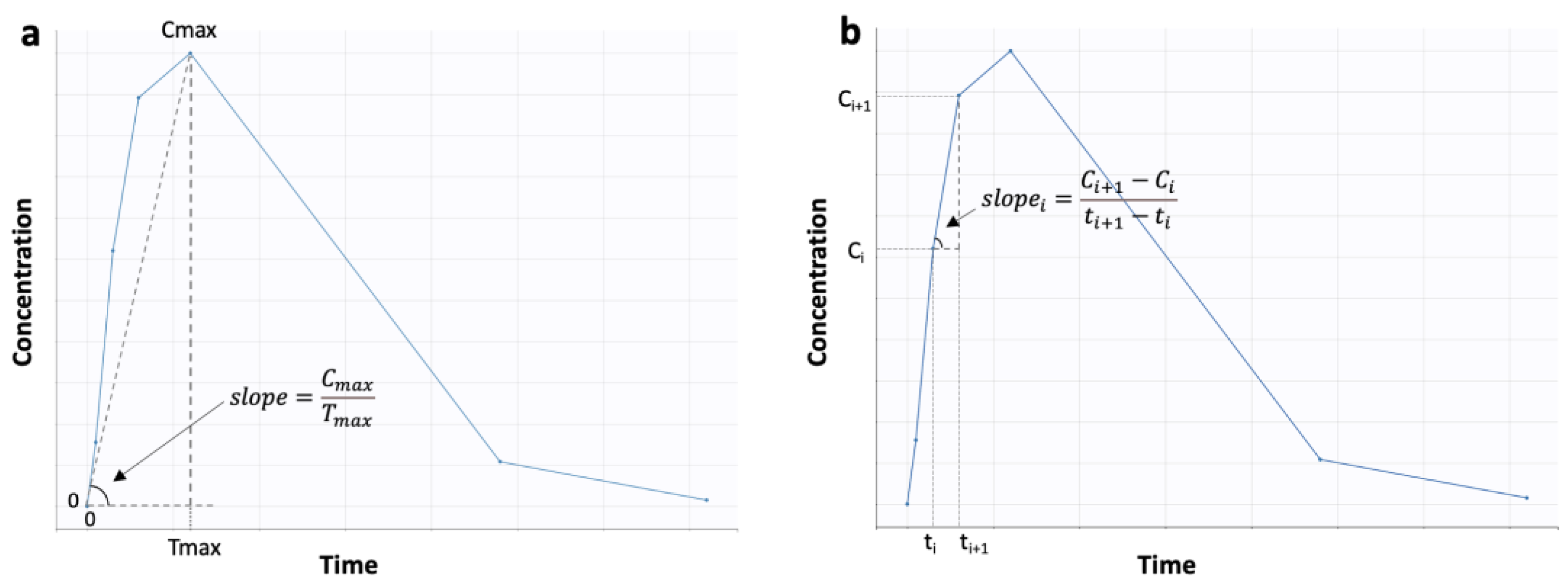
Cmax/Tmax	Ratio of Cmax to Tmax	MATLAB® R2022b (MathWorks)
AS	The “Average Slope” calculated as the average of (C,t) slopes between subsequent time points	MATLAB® R2022b (MathWorks)

summarizes the pharmacokinetic parameters utilized in this study. All these parameters were calculated using model-independent methods (PKanalix^TM, MonolixSuite^TM v2021R2). Among them, there are traditional metrics like AUCt, Cmax, Tmax, the terminal slope (lambda), as well as average concentration (Cavg), the proportion Cmax/Cavg, and the Cmax/AUC ratio, which has been proposed as an indirect measure of the absorption rate. In addition, the partial AUC from time zero up to the median Tmax of the reference product (AUCp) was determined because it has been proposed as a marker of early drug exposure [3].

Apart from the PK parameters outlined above, which have already been proposed in the literature, two more metrics of absorption rate were investigated in this study. The first one is the Cmax/Tmax ratio, which was introduced and explored in a recent study [23]. The latter was found to better reflect the absorption rate compared to all other already-proposed metrics. So, in this study, its properties were further investigated to unveil their properties under more pharmacokinetic conditions (e.g., sampling schemes and absorption rate characteristics).

The Cmax/Tmax ratio actually refers to the tangent of the slope defined by Cmax and Tmax (Figure 1a). A potential limitation of Cmax/Tmax could be the fact that it relies on a single measurement of time (i.e., Tmax) and the corresponding measured concentration (i.e., Cmax). Thus, an alternative estimation method of “slope” is introduced in this study, which utilizes all available C-t data up to Cmax. The new metric, termed “average slope”, is the average of all slopes formed between two consecutive time points (Figure 1b).

The slope (i.e., the tangent) between two sequential time points (times t_i+1 and t_i) can be estimated by the ratio of change in the y-coordinates (i.e., concentration) over the change in the x-coordinates (i.e., time), Equation (1):

$${\mathrm{slope}}_{\mathrm{i}}=\frac{{\mathrm{C}}_{\mathrm{i}+1}-{\mathrm{C}}_{\mathrm{i}}}{{\mathrm{t}}_{\mathrm{i}+1}-{\mathrm{t}}_{\mathrm{i}}}$$

(1)

Thus, the AS (i.e., average slope), which is the mean of these slopes, can be calculated as:

$$\mathrm{AS}=\frac{{{\displaystyle \sum }}_{\mathrm{i}=1}^{\mathrm{n}-1}{\mathrm{slope}}_{\mathrm{i}}}{\mathrm{n}-1}=\frac{{{\displaystyle \sum }}_{\mathrm{i}=1}^{\mathrm{n}-1}\frac{{\mathrm{C}}_{\mathrm{i}+1}-{\mathrm{C}}_{\mathrm{i}}}{{\mathrm{t}}_{\mathrm{i}+1}-{\mathrm{t}}_{\mathrm{i}}}}{\mathrm{n}-1}$$

(2)

where n refers to the number of sampling points up to Tmax. Since there are n points between time zero and Tmax, there are n − 1 intervals that can be used to estimate slope_i. For the purposes of this analysis, a code in MATLAB^® 2022b (MathWorks, Natick, MA, USA) was written for the calculation of AS (Table 1).

In the case of an actual BE study, the AS will be calculated in the typical way of estimating all pharmacokinetic parameters to be in line with the regulatory requirements [2,3]. The AS will be calculated separately for each subject using Equation (2). The estimated AS values will then be ln-transformed, and in these logarithmically transformed values, a general linear model (i.e., ANOVA) will be applied using the appropriate “effects”; namely, in the case of the typical 2 × 2 crossover design, subject (sequence), formulation, sequence, and period. The mean square error of the ANOVA, along with the T/R geometric ratio, will then be used to construct the 90% confidence interval. If both tails of this 90% confidence interval fall within the acceptance limits (typically 80.00–125.00%), the BE can be declared. Obviously, the AS metric can be used in any type of clinical design (e.g., replicate, two-stage, etc.) and statistical method (e.g., scaled limits).

2.4. Simulated Datasets

The population PK estimates used in the current analysis were obtained from a recent publication [23]. In that study, non-linear mixed effect modeling was applied to the actual C-t data of the donepezil BE study (see above). Using the population estimates of parameters and error (between-subject and residual), simulations were performed in order to generate 2 × 2 crossover BE datasets of 1000 subjects each (Simulx^TM, Monolix^TM v2021R2). In addition, three different absorption kinetics were simulated by adjusting the absorption rate constant appropriately: (a) slower absorption by setting the absorption rate constant to half of the original (0.5×), (b) equal to the original (1×), and (c) faster absorption by setting the absorption rate constant to twice the original (2×). All other PK parameters were kept to the actual population pharmacokinetic modeling estimates [23]. The isolation and exploration of absorption kinetics were enabled by changing only the absorption rate constant while leaving the other parameters unchanged.

In addition, three types of sampling schemes were investigated for each case of absorption kinetics: sparse, typical, and dense (

Table 2. Sampling schedules used in the analysis. The sampling schedule for the actual data was the one reported in the study protocol. For the simulated datasets, the “typical” sampling scheme for each absorption kinetic type was designed to characterize the C-t profile appropriately using an optimum number of samples. Sparse designs were developed by omitting sampling points, usually one by one. Dense designs were created by adding sampling points.

Type	Sampling Schedule (in Hours)
Actual dataset
Sampling according to the study protocol	0, 0.5, 1, 2, 3, 4, 6, 8, 12, 24, 48, 96, 144, 192
Simulated datasets
Slow absorption (0.5×)
Sparse	0, 2, 5, 7, 8, 10, 16, 24, 48, 72
Typical	0, 1, 2, 4, 5, 6, 6.5, 7, 7.5, 8, 9, 10, 12, 16, 24, 36, 48, 72
Dense	0, 1, 2, 3, 4, 4.5, 5, 5.5, 6, 6.33, 6.67, 7, 7.33, 7.67, 8, 8.5, 9, 10, 12, 14, 16, 24, 36, 48, 72
Typical absorption (1×)
Sparse	0, 1, 3, 6, 12, 48, 72
Typical	0, 0.5, 1, 2, 3, 4, 6, 8, 12, 24, 48, 72
Dense	0, 0.5, 1, 1.5, 2, 2.33, 2.67, 3, 3.33, 3.67, 4, 4.5, 5, 6, 9, 12, 16, 24, 36, 48, 72
Fast absorption (2×)
Sparse	0, 0.67, 1.25, 1.75, 2.5, 5, 12, 24, 48, 72
Typical	0, 0.33, 0.67, 1, 1.25, 1.50, 1.75, 2, 2.5, 3, 5, 8, 12, 16, 24, 36, 48, 72
Dense	0, 0.33, 0.67, 1, 1.25, 1.50, 1.75, 2, 2.33, 2.67, 3, 3.5, 4, 5, 6, 9, 12, 16, 24, 36, 48, 72

). The use of sampling schemes with varying sampling frequencies allowed investigation of how sensitive the PK parameter calculations were to errors caused by the sampling schedule. The “typical” sampling scheme for each absorption kinetic type (Table 2) was designed to characterize the C-t profile appropriately using an optimum number of samples. Sparse designs were developed by omitting sampling points, usually one by one. Dense designs were created by adding sampling points. In all cases of simulated designs, the last measurement point was set at 72 h, according to the current regulatory guidelines [3].

2.5. Machine Learning Approaches

Machine learning is a subfield of artificial intelligence that uses data and algorithms to mimic how humans learn, gradually improving its accuracy [21,22]. ML is a critical component of the rapidly expanding discipline of data science. In ML, algorithms are taught using statistical approaches to produce classifications or predictions and find critical insights in data mining operations. Two commonly used machine learning algorithms are principal component analysis and random forest.

2.5.1. Principal Component Analysis

PCA is a popular approach for translating a high-dimensional set of features into a low-dimensional set. PCA aims for the lowest-dimensional representation of the data while retaining as much information and variance as possible [21]. PCA turns the original space produced by the original dataset into a new space that is a linear combination of the dataset dimensions in order to capture as much variability as feasible. Each dimension developed is referred to as a principal component. The new data coordinates are referred to as “scores”. Each principal component contributes to the variation in the original data set. The direction of the first principal component is the direction in which the data varies the most.

The “loadings” represent the contribution of each original dimension to the new dimension. The closer the loading value is to +1 (or −1), the higher the positive (or negative) impact of the feature on this principal component. Loadings are represented by arrows that are at an angle and have a specific length. The angle represents a specific feature’s contribution in the direction of the principal component, where it contributes. The length of the arrow represents the strength of the feature’s contribution in that direction. A loading plot depicts the strength with which each attribute influences a major component.

The “biplot” is another method for examining the loadings and scores together. The biplot is a two-dimensional scatter plot with two axes corresponding to the two most important components in terms of explained variance. In this two-dimensional coordinate system, the loadings of the first two principal components of each characteristic are presented across the data points, using the scores as coordinates.

Scree plots are used to determine the fewest number of major components required to adequately represent the original data. The primary goal of a scree plot is to illustrate the results of the component analysis and to locate the apparent change in slope (the elbow). In a scree plot, the eigenvalue is shown against the principal components. The proportion of variance explained by a component is calculated by dividing its eigenvalue by the total of its eigenvalues. The initial component usually explains a significant percentage of the variability, the successive components explain a moderate portion, and the final components explain only a small portion of the total variability. In this study, the PCA analysis was carried out using Python v. 3.10.8. The package “matplotlib” was used to construct statistical plots, while the PCA analysis was implemented using the libraries “seaborn”, “sklearn”, and “bioinfokit”.

2.5.2. Random Forest

The random forest is a supervised classification technique made up of several decision trees. When building each individual tree, it employs bagging and feature randomness in an attempt to produce an uncorrelated forest of trees whose forecast for the target variable is more precise and consistent than that of any individual tree [21]. Prior to utilizing RF, the response (target) variable had to be in the form of an ordinal scale. Thus, in this study, Tmax estimates were changed from their original continuous scales to ordinal scales. The most reasonable approach was to categorize each variable into quartiles. Then, four groups with an equal number of observations each were constructed, providing a balanced representation of all attributes: very high, high, medium, and low variable values.

The “confusion matrix” is used to evaluate the performance of a model in a classification exercise where the dependent variable is categorical. The confusion matrix is an M × M matrix, where M denotes the number of response variable classes. The matrix contrasts between the expected and true classes. This gives a comprehensive view of the categorization model’s overall performance as well as the types of errors it makes. It is also possible to investigate the feature importance when using the random forest to determine the contribution of each variable to the prediction of the response variable. The random forest algorithm was implemented in Python v.3.10.8 using, among others, the packages “sklearn”, “matplotlib”, “kneed”, “tqdm”, “math”, and “seaborn”.

The overall actions, purposes, and software used in this study are listed in

Table 3. A summarized outline of actions, their purposes, and the software used for their implementation.

Step	Action	Purpose	Software
Actual dataset
1	Parameters estimation	Calculation of pharmacokinetic parameters (see Table 1) in order to apply, in a subsequent step, the machine learning techniques	- PKanalixTM (Monolix SuiteTM 2021R2) - MATLAB® R2022b (MathWorks)
2	PCA	Application of Principal Component Analysis (PCA) in order to identify relationships among the parameters	- Python v. 3.10.8
3	RF	Application of Random Forest (RF) in order to explore the relative contribution of pharmacokinetic parameters to Tmax	- Python v. 3.10.8
4	Pharmacokinetic simulations	Perform pharmacokinetic simulations in order to generate 2 × 2 crossover bioequivalence datasets for several absorption kinetics (slow, typical, fast) and sampling schemes (sparse, typical, dense)	- SimulxTM (Monolix SuiteTM 2021R2)
Simulated datasets (Steps 1–3 are repeated for each simulated dataset)
5	Parameters estimation	Calculation of pharmacokinetic parameters	- PKanalixTM (Monolix SuiteTM 2021R2) - MATLAB® R2022b (MathWorks)
6	PCA	Application of PCA in order to identify relationships among the parameters	- Python v. 3.10.8
7	RF	Application of RF in order to explore the relative contribution of pharmacokinetic parameters to Tmax	- Python v. 3.10.8

Key: PCA, Principal Component Analysis; RF, Random Forest.

.

3. Results

3.1. Actual Data

3.1.1. Relationships among the Pharmacokinetic Parameters

PCA was performed in order to extract information from the study individuals and investigate the correlations among the PK variables (Figure 2). The observations are represented by dots in the plane generated by the two initial main components, while the lines refer to the vectors of the variables (e.g., Cmax, AUCt, average slope, Cmax/Tmax, etc.). The loading scores (l1 and l2) of the first and second principal components are shown next to the PCA plot. Overall, the first and second major components account for 73.85% of the overall variability, where 49.99% and 23.86% come from the first and second principal components, respectively.

Figure 2 shows that AUCt and AUCinf are superimposed on the upper right side of the plot, both sharing almost the same l1 value (0.21 and 0.20, respectively). Partial AUC and Cavg also show exactly the same behavior. In the same vein, the newly introduced terms AS and Cmax/Tmax represent very similar performance, with both of them exhibiting quite similar l1 values (0.39 and 0.38, respectively). Among the other variables, Cmax (l1 = 0.32, l2 = 0.18) lies between the previously mentioned clusters of parameters, namely between the (AUCt, AUCinf) and the (AS, Cmax/Tmax) vectors. Tmax, which is currently considered the parameter best expressing the kinetic properties of absorption, is located at the upper left part of the PCA plot. Next to Tmax, can be found the ratio Cmax/Cavg exhibited an l1 score of −0.26 and l2 equal to 0.10. The terminal slope (lambda) shows a completely different behavior compared to the other PK parameters, being the only one found in the third quadrant.

It is worth mentioning that the AS (or Cmax/Tmax) vector is antidiametric to Tmax (the angle between them is close to 180 degrees). In particular, the angle ∠(AS·0·Tmax) is equal to the sum of the inverse cosines, namely, arccos(l1_Tmax) + arccos(l1_AS) = arccos(−0.27) + arccos(0.39) = 105.6° + 67.0° = 172.6°. This attribute implies the opposite kinetic behavior between AS and Tmax. In other words, as AS gets higher, namely due to faster absorption, Tmax becomes lower, i.e., it appears at earlier time points. Thus, AS succeeds in expressing the kinetic character of absorption. This attribute is not observed for Cmax since the angle between Cmax and Tmax is much less than 180 degrees.

Scree plots were created to determine the optimal number of primary components (Figure 3). The y-axis displays the eigenvalues (percentage of variance explained), while the x-axis displays the number of components. The scree plot criterion looks for the “elbow” of the curve and selects all components just before the line flattens out. Based on the scree plot shown in Figure 3, the initial two principal components were selected.

3.1.2. Parameters Contributing to Tmax

The PCA analysis presented above enabled the detection of the relationship among all PK parameters, placing particular interest on Tmax. The random forest approach was further used to determine the contribution of each PK feature to Tmax. The latter was accomplished in two ways: first, by including the Cmax/Tmax term in the model alongside the other PK parameters, and second, by substituting the AS for Cmax/Tmax. Since RF is a supervised technique and the response variable should be on an ordinal scale, prior to its application, the Tmax estimates were transformed into an ordinal scale. A common way to do this was to divide Tmax into its quartiles, thus creating four groups with an equal number of elements. The four classes of Tmax refer to low, medium, high, and very high values. These quartile values were found to be two, three, and four for the 1st, 2nd (i.e., the median), and 3rd quartile, respectively.

Figure 4 depicts the application of the RF algorithm either by using Cmax/Tmax (Figure 4a) or AS (Figure 4b). The reason for not including both Cmax/Tmax and AS in the same model is due to their similar natures, and it was attempted to isolate the effect of each one of them on Tmax. The RF results showed that in both cases, the major contributor to Tmax was AS (or Cmax/Tmax), followed by AUCp, AUCt, Cmax/AUC, Cmax, and finally, lambda. It is worth noting that Cmax, which is traditionally used in BE studies as the metric expressing absorption rate, shows a low contribution to Tmax, even less than that of AUCt. The Cmax/AUC ratio, which has also been proposed as a metric to express the rate of absorption, also shows a low contribution to Tmax. Based on the two confusion matrix results, the prediction accuracy is 79.82% for the RF model of Figure 4a and 81.03% for that of Figure 4b. Finally, it should be mentioned that AUCinf was not included in the RF analysis since it shows exactly the same properties as AUCt.

3.2. Simulated Datasets

The goal of the last part of the investigation was to explore the performance of AS (and Cmax/Tmax), as well as the other PK measures, under various kinetic scenarios. To achieve this goal, simulations were performed with absorption rates that were faster (2×), slower (0.5×), and equal (1×) to the actual absorption rate. Thus, simulated 2 × 2 crossover BE datasets, with N = 1000 subjects each, were generated, and machine learning was applied to them. The remaining population pharmacokinetic parameters were those obtained through non-linear mixed effect modeling and reported in the Karalis 2023 study [23]. In addition, the three kinetic conditions (slow, typical, and fast) were combined with the three sampling schemes (see Table 2). Overall, nine conditions of BE studies were simulated, and the simulated C-t data for these datasets are depicted in Figure 5. The impact of the sampling scheme is highlighted in Figure 5a, where the absorption rate constant is set equal to the typical estimate from the population pharmacokinetic modeling. The role of absorption rate can be seen in Figure 5b, where the C-t profiles generated from three levels of absorption rate constant are shown in the case of the “typical” sampling scheme. Using different sampling schemes (i.e., with different sampling densities) allows exploring the impact of the dataset on the estimation of the PK parameters and mainly on the estimation of single point parameters like Cmax, Tmax, and Cmax/Tmax. Following that, all PK parameters (see Table 1) for each scenario were calculated, and the analysis was continued by re-applying the two ML algorithms (PCA and RF) on each BE dataset.

3.2.1. Relationships among the PK Parameters

In order to identify the relationships among the PK parameters, PCA was performed on the simulated BE datasets. In order to facilitate the clarity of the plots, PK parameters of secondary importance, like Cavg and Cmax/Cavg, were excluded from this analysis. Figure 6 shows the biplots for the three sampling schemes: sparse (Figure 6a), typical (Figure 6b), and dense (Figure 6c). In all three cases, almost similar results were obtained. Additionally, the findings from the simulated datasets are in line with those derived from the actual donepezil data (Figure 2). AS and Cmax/Tmax show similar performances (they are superimposed) and are almost the opposite of Tmax (the angle formed between them is close to 180°). This attribute remains constant regardless of the type of sampling scheme and verifies the opposite behavior between AS (or Cmax/Tmax) and Tmax. The latter underlines the desired characteristics of the two newly proposed metrics (AS and Cmax/Tmax) for the rate of absorption. The descriptive ability of the PCA models is equal to 75.24% for the sparse case (Figure 6a), 73.30% for the typical case (Figure 6b), and 78.02% for the sparse design (Figure 6c). Two principal components were identified in all three cases, and the scree plots are depicted in Figure A1 in the Appendix A.

To focus on the role of the sampling scheme, which may have the greatest influence on the calculation of Cmax and Tmax, the simulated data were divided into three categories: sparse, typical, and dense. In each category, the simulated data of the scenarios with different absorption kinetics were merged. The PCA results presented above refer to each pre-referred dataset. Furthermore, in Figure A2, Figure A3 and Figure A4 of the Appendix A, PCA analyses are shown separately for each absorption scenario.

3.2.2. Parameters Contributing to Tmax

The PCA provided above enabled the discovery of a link between all PK parameters, particularly Tmax. The random forest method was then utilized to explore the contribution of each PK characteristic to Tmax. As in the case of actual data, the latter was accomplished separately using either AS or Cmax/Tmax. The Tmax estimates for each dataset were transformed into an ordinal scale by splitting into the corresponding quartiles of distribution (

Table A1. Median and quartile values of the Tmax estimates. (A) The upper panel shows the median Tmax values for the calculation of partial AUC (i.e., AUCp) in the case of simulated datasets referring to slow, typical, and fast absorption. (B) The lower panel lists the Tmax quartile values of the merged datasets (i.e., when all kinds of absorption kinetics are combined) for the sparse, typical, and dense sampling schedules. The quartile values of panel “B” were used for the deployment of random forest models.

A. Individual Datasets
Type of absorption kinetics and sampling scheme	Median of Tmax (in hours)
Slow absorption
Sparse	7.00
Typical	6.50
Dense	6.00
Typical absorption
Sparse	3.00
Typical	3.00
Dense	2.50
Fast absorption
Sparse	1.75
Typical	1.75
Dense	1.75
B. Merged datasets
Type of sampling scheme	Quartiles of Tmax (in hours) (1st, 2nd, 3rd)
Sparse	1.75, 2.50, 6.00
Typical	1.75, 2.75, 6.00
Dense	1.75, 2.67, 5.00

in the Appendix A). Since the response variable (Tmax) was on an ordinal scale, the supervised RF method was able to be applied.

Figure 7 depicts the application of the RF algorithm when the Cmax and Tmax are used. Three different conditions are analyzed depending on the sampling scheme (see Table 2) utilized, namely, sparse sampling (Figure 7a), typical sampling (Figure 7b), and dense sampling (Figure 7c). The left side of the graph refers to the variable importance of each PK parameter, while the plot on the right is the confusion matrix showing the predicting accuracy of the developed RF model.

Regardless of the sampling design, all RF results coincided and showed that the major contributor to Tmax is always Cmax/Tmax. Lambda and AUCt, which represent elimination and absorption extent, made the least contribution. Then, depending on the sampling scheme, different performance was observed for the other metrics. For example, in the case of a sparse scheme, Cmax was the second-most important contributor (after Cmax/Tmax), followed by AUCp and Cmax/AUC. For the cases of typical and dense sampling schemes, the ratio Cmax/AUC exhibited a greater contribution compared to Cmax and AUCp. The confusion matrices showed high prediction accuracy for all three models, namely, 89.80% for the sparse sampling case (Figure 7a), 80.77% for the typical (Figure 7b), and again 80.77% (but with different individual values) for the dense design (Figure 7c).

Figure 8 depicts the application of the RF algorithm when AS is used instead of Cmax and Tmax for the three scenarios of sampling schemes: sparse (Figure 8a), typical (Figure 8b), and dense (Figure 8c). The results obtained for AS are almost identical to those found above in the case of Cmax and Tmax. Again, the sampling frequency did not affect the behavior of AS, which was always found to be the major contributor to Tmax. All other PK parameters exert a lesser contribution to Tmax. Additionally, the prediction accuracy is high for the three RF models and equal to 83.67%, 73.08%, and 76.92% for the sparse, typical, and dense designs, respectively.

4. Discussion

The purpose of this study was to introduce “average slope” as a new metric characterizing the “rate” of absorption and explore its properties compared to other metrics using ML approaches. The advantages of using AS, as an absorption metric are proven through a stepwise procedure of applying machine learning approaches. In order to tackle the challenge of defining a new absorption rate measure, this study exploits tools from the fields of machine learning and population pharmacokinetic modeling. Initially, the analysis was performed on actual data from a BE study of donepezil in 26 healthy volunteers. Additionally, using a previously developed population pharmacokinetic model [23], simulated two × two crossover BE datasets were generated for combinations of three sampling schemes (sparse, typical, and dense) with different absorption kinetics (slow, typical, and fast). This way of analysis allowed exploring the properties of the newly proposed parameter (average slope) along with the other PK parameters under several scenarios. The study path was planned to be similar to a “screening process”, with each exploration stage revealing some aspects of the PK metrics, allowing the optimal absorption metric to be determined gradually. The scenarios provided a progressive strategy to exclude PK parameters from their usage as absorption rate measures.

A summarized view of the main findings is shown in

Table 4. The stepwise process of analysis allowed screening the pharmacokinetic parameters with the desired behavior. Within each step of the analysis, the pharmacokinetic parameters are listed in the order of preference (>).

Step	Action	Order of Preference	Parameters with Non-Desired Characteristics
Actual dataset
1	PCA	AS or Cmax/Tmax > Cmax/AUCt > AUCp or Cavg	Cmax, Cmax/Cavg, lambda, AUCt, AUCinf
2	RF	AS or Cmax/Tmax > AUCp	AUCt, Cmax/AUC, Cmax, lambda
3	Overall	Best performance: AS or Cmax/Tmax and afterwards AUCp
Simulated datasets
4	PCA	AS or Cmax/Tmax > Cmax/AUC	AUCt, AUCinf, Cmax, AUCp, lambda
5	RF	AS or Cmax/Tmax	AUCt, Cmax, AUCp, Cmax/AUC, lambda
6	Overall	Best performance: AS or Cmax/Tmax
Overall findings from steps 1–3 and 4–6
7	Overall from the entire analysis	Best performance: AS or Cmax/Tmax	All other parameters tested

Key: PCA, Principal Component Analysis; RF, Random Forest.

. The application of PCA to the actual data allowed the identification of AS (followed by Cmax and Tmax) as the most desired behavior because it performs almost oppositely to Tmax (Figure 2). This attribute is desired since it shows that AS reflects the kinetic character of absorption; as the AS increases, Tmax occurs at earlier time points. Based on the PCA results, other PK metrics (like AUCp and Cmax/AUC) could probably reflect the kinetic behavior, but to a lesser extent. However, according to the findings from the RF model (Figure 4), it became obvious that Cmax/AUC, which has been proposed as a possible indirect measure of absorption, contributes to a low extent to Tmax. In the same RF model, AUCp appears to exert a relatively high contribution, and it is the second most important after AS (or Cmax/Tmax). Thus, the initial application of the two machine learning techniques to the actual BE data filtered out the PK metrics for expressing the absorption rate. Up to this point, the potential PK measures could be: primarily AS (or Cmax/Tmax) and secondarily AUCp. All other parameters should be omitted since they did not find a way to express the desired properties.

The next step was to use simulated data to look into more possible situations. To simulate situations with different absorption kinetics (slow, typical, fast) and sampling procedures (sparse, typical, dense), a population pharmacokinetic model from a previous study was used [23]. For the case of different absorption kinetics, all donepezil parameters (as well as the estimated between- and within-variabilities) were kept identical to those found from the population pharmacokinetic analysis, while only the absorption rate constant changed. The latter aimed to isolate the impact of the absorption rate from the other aspects of the PK performance (e.g., distribution and elimination properties). Furthermore, the use of sampling schemes with different sampling frequencies (Table 2) allowed us to investigate how sensitive to errors (due to the sampling schedule) the calculations of the PK parameters are, particularly for Cmax/Tmax, Tmax, and Cmax, which are based on a single time point measurement. Since for ML, a large number of cases is preferred, the simulated number of subjects was set equal to 1000 per study.

Application of PCA to the simulated data verified the findings observed above in the case of actual data. The opposite performance of AS (or Cmax/Tmax) compared to Tmax was consistent for all the different scenarios studied. For AUCp, a variable performance was observed; in some cases, such as the simulated “typical” case (Figure 6b), the results were similar to those from the actual data, and AUCp showed a desired performance. However, the behavior of AUCp was not desired for the cases of sparse (Figure 6a) or dense (Figure 6c) sampling schemes. On the contrary, the ratio Cmax/AUC expressed a nice performance in all these scenarios. In the subsequent step, the application of RF models to the simulated data further clarified these findings. In particular, it was shown that the major contributor to Tmax is always AS (or Cmax/Tmax). The next most important contributors (but with a much lower contribution compared to AS or Cmax/Tmax) were either Cmax or Cmax/AUC. However, Cmax/AUC showed low importance for Tmax when sparse sampling schemes were utilized. Besides, Cmax has already been excluded from the PCA analysis, whether in the actual or simulated data (Table 4). It is also worth noting that the partial AUC (i.e., AUCp) until the median Tmax of R, which is currently used as an early exposure metric in regulatory guidelines [2,3], fails to characterize the kinetic manner of absorption. The latter can be derived from the PCA analysis applied to the simulated data. The moderate-to-low contribution of AUCp to Tmax observed in the RF models further adds to its undesirable character. Overall, it appears that only AS (or Cmax/Tmax) exhibits the desired performance in all cases for either the PCA or RF models (Table 4). AS and Cmax/Tmax appear superior to all other PK parameters in terms of reflecting absorption rate. For “slow” absorption kinetics (Figure A3a and Figure A4a), AS shows slightly better behavior compared to Cmax/Tmax.

Apart from the findings offered by the two machine learning approaches, there is also a fundamental theoretical reason for considering a parameter as a measure of the absorption rate. This essential issue refers to the units of measurement. A parameter that is used to express the “rate” of a process should represent the change of a measure (e.g., distance, concentration, etc.) over time. In the case of absorption, since we are not able to know the absolute quantities after oral administration of a drug, an appropriate measure of absorption rate should have units of concentration per time. That means that this measure should be the ratio of the change in drug concentration values divided by the relevant change in time (Equation (3)).

$$\mathrm{Rate} \mathrm{of} \mathrm{absorption}=\frac{\mathrm{Change} \mathrm{in} \mathrm{drug} \mathrm{concentration}}{\mathrm{Change} \mathrm{in} \mathrm{time}}$$

(3)

It becomes evident that all other metrics proposed in the literature do not exhibit the appropriate units. The several expressions of areas under the curve (AUCt, AUCp, AUCinf) refer to surfaces and have units of concentration·time. Therefore, these measures should be used to reflect several aspects of the extent of absorption. It should not be disregarded that AUCp has been proposed as a measure to express early “exposure” and not the rate of absorption. Besides Cmax, which is traditionally used in BE studies as an indirect metric for absorption rate, there is only one concentration measurement. As a result, in principle, it cannot be used to express the rate. Even though Cmax is currently used worldwide to indirectly reflect absorption rate, the machine learning findings presented in this study disputed this fact, showing that there is a small direct relationship with Tmax (Figure 2 and Figure 4). The ratio Cmax/AUC has been proposed as an alternative to Cmax, aiming to exclude the influence of absorption extent by dividing with AUCt; however, Cmax/AUC lacks appropriate units because it is the fraction concentration/(concentration time) = time⁻¹. The concept of “intercept” on the axis of the relative concentration values has also been proposed [17,18]. In this case, the absorption rate metric is determined by dividing the initial concentrations of the drug in the two formulations by the time point [17]. A different approach to the “intercept” concept was the “Modified Intercept” metric, which utilized the limit of the quotient C/t when t→0 (i.e., the intercept on the axis of concentration) [18]. However, these approaches assume first-order kinetics, a one-compartment model, and are based on complex estimation methods since they require log transformation, application of linear regression analysis, back extrapolation to time zero, and estimation of the intercept. Finally, Tmax, which has been considered an appropriate measure to express the rate of bioequivalence, has not been used because it is on a discrete scale and lacks appropriate measurement units [24]. Tmax has units of time, and therefore it cannot, in principle, be used to express the absorption rate.

The simplest approach to fulfilling the requirements of Equation (3) is through the use of Cmax/Tmax, which refers to the slope formed between the (Tmax, Cmax) coordinates, namely, the tangent of the angle ∠(Cmax·0·Tmax) (Figure 1a). In order to avoid using a metric that relies on a single measurement (since both Cmax and Tmax come from the same measurement), an alternative approach is introduced in this study that is termed “average slope”. The latter is calculated as the average of all slopes between subsequent time points up to Tmax (Figure 1b). AS or Cmax/Tmax have the appropriate concentration/time units and express rate of change.

As mentioned above, one of the benefits of using AS instead of Cmax/Tmax is that AS estimation is based on many points and is easy to figure out by using a model-independent approach. Another advantage of using AS is that it can be thought of as a generalization of Cmax/Tmax, as shown in Equations (4)–(8).

We can calculate the sum of slopes using the AS definition from Equation (2), and we get:

$$\mathrm{Sum} \mathrm{of} \mathrm{slopes}={\displaystyle \sum }_{\mathrm{i}=1}^{n-1}\frac{{\mathrm{C}}_{\mathrm{i}+1}-{\mathrm{C}}_{\mathrm{i}}}{{\mathrm{t}}_{\mathrm{i}+1}-{\mathrm{t}}_{\mathrm{i}}}={\displaystyle \sum }_{\mathrm{i}=1}^{\mathrm{n}-1}\frac{{\mathrm{C}}_{\mathrm{i}+1}-{\mathrm{C}}_{\mathrm{i}}}{{\mathsf{\Delta }\mathrm{t}}_{\mathrm{i}}}$$

(4)

where Δt_i refers to the sampling interval at time i.

In the special case where the sampling interval is constant (Δt_i = Δt), at least for times up to Tmax, Equation (4) can be re-written:

$$\mathrm{Sum} \mathrm{of} \mathrm{slopes}={\displaystyle \sum }_{\mathrm{i}=1}^{\mathrm{n}-1}\frac{{\mathrm{C}}_{\mathrm{i}+1}-{\mathrm{C}}_{\mathrm{i}}}{\mathsf{\Delta }\mathrm{t}}$$

(5)

By eliminating the consecutive concentration values, we get:

$$\mathrm{Sum} \mathrm{of} \mathrm{slopes}=\frac{{\mathrm{C}}_{\mathrm{n}}}{\mathsf{\Delta }\mathrm{t}}$$

(6)

where C_n is the last measured concentration up to the occurrence of the maximum, namely; that C_n refers to Cmax. In order to calculate AS from Equation (6), we have:

$$\mathrm{AS}=\frac{\mathrm{Sum} \mathrm{of} \mathrm{slopes}}{\mathrm{number} \mathrm{of} \mathrm{intervals}}=\frac{{\mathrm{C}}_{\mathrm{n}}}{\mathrm{n}-1}=\frac{{\mathrm{C}}_{\max }}{\mathsf{\Delta }\mathrm{t} \times \left(\mathrm{n}-1\right)}$$

(7)

The product Δt·(n − 1) refers to Tmax, thus:

$$\mathrm{AS}=\frac{{\mathrm{C}}_{\max }}{{\mathrm{T}}_{\max }}$$

(8)

Therefore, in the special case of equally spaced sampling intervals, AS becomes identical to Cmax/Tmax. When the sampling intervals are not equal, which is more realistic in actual BE studies, then AS (Equation (2)) offers the advantage of providing an estimation of slope based on many points (Figure 1b). In other words, AS is less dependent on the specific time point of Tmax, and therefore it is less influenced by its failure to accurately detect it due to sparse sampling.

In the previous study [23], the Cmax/Tmax ratio was found to be a metric expressing the rate of absorption. Its properties have been assessed and compared to other PK parameters using machine learning. In that study, it was found that Tmax was the major contributor to Cmax/Tmax irrespective, of absorption kinetics. The current analysis extends previous findings by introducing the new metric, average slope, which is a generalization of Cmax/Tmax, and performing more simulations and machine learning analyses. The new metric, AS, succeeds in expressing the kinetic properties of absorption both conceptually (i.e., with the appropriate units and physical meaning) and in practice, namely, from the machine learning results. It should be underlined that AS can be easily calculated by applying a model-independent method using the average of the subsequent slopes (see Equation (2)). Additionally, it does not require any assumptions (e.g., first-order kinetics), any model (e.g., one- or two-compartment), or transformations. The estimation method of AS is as simple as that of the widely used AUCt in the case of the extent of absorption.

In pharmacokinetics, the typical C-t profile (Figure 1) observed after oral administration is the result of three processes occurring concomitantly in the body: absorption, distribution, and elimination. Absorption dominates in the early time points, namely during the rapid increase in concentration values, while there is an equilibrium between the three processes as time passes. The time point where there is an equilibrium, namely the input rate (i.e., absorption rate), becomes equal to the output (i.e., elimination and/or distribution to tissues) refers to Tmax. Thus, in order to place more emphasis on absorption kinetics, a modified version of AS can also be defined. In this context, the weighted average slope (AS_w) (Equation (9)) can be defined by appropriately modifying AS (i.e., Equation (2)):

$${\mathrm{AS}}_{\mathrm{w}}=\frac{{{\displaystyle \sum }}_{\mathrm{i}=1}^{\mathrm{n}-1}\left(\frac{\mathrm{Tmax}-{\mathrm{t}}_{\mathrm{i}}}{\mathrm{Tmax}}\times {\mathrm{slope}}_{\mathrm{i}}\right)}{\mathrm{n}-1}=\frac{{{\displaystyle \sum }}_{\mathrm{i}=1}^{\mathrm{n}-1}\left(\frac{\mathrm{Tmax}-{\mathrm{t}}_{\mathrm{i}}}{\mathrm{Tmax}}\times \frac{{\mathrm{C}}_{\mathrm{i}+1}-{\mathrm{C}}_{\mathrm{i}}}{{\mathrm{t}}_{\mathrm{i}+1}-{\mathrm{t}}_{\mathrm{i}}}\right)}{\mathrm{n}-1}$$

(9)

The unitless weighting factor (Tmax − T_i)/Tmax places more weight on earlier time points where the effect of absorption is predominant, and therefore AS_w can express more purely the absorption process. As in the case of AS, the estimation of AS_w is model-independent, and no assumptions are required for its calculation. Even though more studies are required to examine all properties of AS and AS_w, it is a regulatory criterion to select between AS and AS_w; namely, if we need a metric placing emphasis on all points up to Tmax (i.e., AS) or a metric (i.e., AS_w) that is influenced more by the early time points, which are more indicative of absorption.

The current study used simulated data to investigate different absorption rates (slow, typical, and fast) and sampling schemes (sparse, typical, and dense). A special emphasis was placed on the sampling schedule (Table 2) since the appropriate identification of Tmax depends on the appropriateness of the sampling schedule around Cmax. Even though the utilized sampling scheme is generally termed “sparse”, “typical”, and “dense”, they were different among the conditions tested; in other words, they were appropriately set to fit in the absorption kinetic scenario (see Table 2).

It should be noted that, for the sake of this research, the donepezil population PK model developed in the previous study [23] was utilized to generate several two × two crossover simulated BE datasets. The use of simulated datasets allowed us to verify earlier findings and investigate the influence of absorption rate on each metric. This method has the advantage of preserving all donepezil PK parameters at the same level as the original dataset while only the absorption rate constant is changed. As a result, the impact of the absorption rate could be identified and analyzed in the machine learning analysis. Setting the absorption rate constant at “0.5×” and “2×” of the initial estimate is considered a reasonable choice for slower and quicker absorption, respectively (Figure 5). Slower or quicker absorption kinetics than those described above would not provide any advantage or alter the results. Furthermore, the use of simulated conditions for the actual data (i.e., the “1×” scenario) allowed the findings acquired from the original dataset to be validated. It is worth mentioning that the random forest analysis implemented in this study was carried out in a way to explore the PK parameters’ contribution to Tmax, namely, in the opposite way of what was done in the previous study.

Overall, in this study, AS is introduced as a new metric for characterizing the absorption rate. AS has several advantages over the traditionally used Cmax and the previously proposed Cmax/Tmax. These advantages are briefly outlined below:

(a) AS satisfies the fundamental theoretical reason for considering a parameter as a measure of absorption rate; namely, AS has units of concentration/time in contrast to all other measures proposed in the literature, which have meaningless units.

(b) The machine learning methods applied in this study showed that AS succeeds in reflecting the “absorption rate”, while Cmax and other existing metrics fail.

(c) AS can be estimated quite simply using a model-independent approach (Equation (2)), as in the case of AUCt, without any assumptions.

(d) AS is a generalization of Cmax/Tmax, and therefore AS can be applied to either equally or unequally spaced (as they usually exist in practice) sampling schemes.

(e) Due to the calculation of AS, which relies on many data points, estimation bias that might occur to Cmax/Tmax can be avoided in the case of AS.

(f) Finally, the weighted version of AS (i.e., AS_w) allows more emphasis to be placed on early time points, thus expressing more purely the absorption process.

A limitation of this study is that the machine learning methods were only applied to one actual BE dataset. Even though several simulated datasets were constructed and studied, to circumvent this constraint, the additional use of actual BE datasets is required. Additionally, more research on the performance of the PK measures in more drugs with variable pharmacokinetics, particularly absorption kinetics, is needed. Additional work is needed to explore the sensitivity and specificity of the new metric, AS, under several absorption kinetics scenarios. In this context, it would be necessary to quantify type I (1—specificity) and type II (1—power) errors of AS and AS_w, using the traditional method of Monte Carlo simulations. Many modeling studies are required to examine all possible scenarios of absorption (e.g., lag time, parallel absorption, Erlang-type, multiple transit compartments, double peaks, etc.), as has been done in the past for other metrics [20]. In this study, machine learning was applied to reveal the properties of AS in a way that has not been done before. In addition, studies with large sample sizes or merging different studies should be applied in order to increase the data input and facilitate the ML algorithms to get robust estimates. In this study, to address the problem of low data entry, the simulated data consisted of N = 1000 subjects under each scenario.

5. Conclusions

The concept of “average slope” is introduced in this study as a metric to express the absorption rate that can be used as a primary endpoint in BE studies. Two machine learning methods, principal component analysis and random forest models, were applied to actual and simulated bioequivalence data in order to uncover the properties of AS and show that AS expresses the appropriate properties for characterizing absorption rate. Several absorption kinetics (slow, typical, fast) and sampling schemes (sparse, typical, dense) were simulated in order to investigate many different conditions and their impact on the performance of all pharmacokinetic parameters. The two machine learning algorithms, applied to all these scenarios, proved the desired properties of AS to characterize absorption rate while showing the non-desired performances of other metrics currently used (i.e., Cmax) or have been proposed in the literature (e.g., Cmax/AUC, AUCp). AS meets the fundamental theoretical reason for adopting a parameter as a measure of absorption rate; notably, AS has concentration/time units, as opposed to all other measures offered in the literature, which have meaningless units. This study also provides a model-independent estimation method for AS, as well as a theoretical justification for its suitability to express absorption rate. The estimation of AS does not require any assumptions, models, or transformations and is as simple as that of AUCt, which is widely used in pharmacokinetics and bioequivalence studies. In addition, a modified version of AS, the so-termed weighted AS, is introduced and can be used to place emphasis on early time points, where the C-t profile describes more clearly the absorption process. Overall, the modern machine learning technique, used within pharmacokinetics and bioequivalence assessment, enabled the exploration of an old problem and the provision of a solution.

References

- Niazi, S. Handbook of Bioequivalence Testing (Drugs and the Pharmaceutical Sciences), 2nd ed.; CRC Press, Taylor & Francis Group: Boca Raton, FL, USA, 2014. [Google Scholar]
- Food and Drug Administration (FDA). Guidance for Industry. Bioavailability and Bioequivalence Studies Submitted in NDAs or INDs-General Considerations. Draft Guidance. U.S. Department of Health and Human Services Food and Drug Administration Center for Drug Evaluation and Research (CDER). December 2013. 2014. Available online: https://www.fda.gov/media/88254/download (accessed on 4 January 2023).
- European Medicines Agency. Committee for Medicinal Products for Human Use (CHMP). Guideline on the Investigation of Bioequivalence. CPMP/EWP/QWP/1401/98 Rev. 1/ Corr**. London. 20 January 2010. Available online: https://www.ema.europa.eu/en/documents/scientific-guideline/guideline-investigation-bioequivalence-rev1_en.pdf (accessed on 4 January 2023).
- Bois, F.; Tozer, T.; Hauck, W.; Chen, M.; Patnaik, R.; Williams, R. Bioequivalence: Performance of several measures of extent of absorption. Pharm. Res. 1994, 11, 715–722. [Google Scholar] [CrossRef] [PubMed]
- Reppas, C.; Lacey, L.F.; Keene, O.N.; Macheras, P.; Bye, A. Evaluation of different metrics as indirect measures of rate of drug absorption from extended-release dosage forms at steady-state. Pharm. Res. 1995, 2, 103–107. [Google Scholar] [CrossRef] [PubMed]
- Endrenyi, L.; Tothfalusi, L. Metrics for the evaluation of bioequivalence of modified-release formulations. AAPS J. 2012, 14, 813–819. [Google Scholar] [CrossRef] [PubMed]
- Jackson, A. Determination of in vivo bioequivalence. Pharm. Res. 2002, 19, 227–228. [Google Scholar] [CrossRef] [PubMed]
- Chen, M.; Lesko, L.; Williams, R. Measures of exposure versus measures of rate and extent of absorption. Clin. Pharmacokinet. 2001, 40, 565–572. [Google Scholar] [CrossRef] [PubMed]
- Basson, R.; Cerimele, B.; DeSante, K.; Howey, D. Tmax: An unconfounded metric for rate of absorption in single dose bioequivalence studies. Pharm. Res. 1996, 13, 324–328. [Google Scholar] [CrossRef] [PubMed]
- Rostami-Hodjegan, A.; Jackson, P.; Tucker, G. Sensitivity of indirect metrics for assessing “rate” in bioequivalence studies: Moving the “goalposts” or changing the “game”. J. Pharm. Sci. 1994, 83, 1554–1557. [Google Scholar] [CrossRef] [PubMed]
- Schall, R.; Luus, H. Comparison of absorption rates in bioequivalence studies of immediate release drug formulations. Int. J. Clin. Pharmacol. Ther. Toxicol. 1992, 30, 153–159. [Google Scholar] [PubMed]
- Endrenyi, L.; Al-Shaikh, P. Sensitive and specific determination of the equivalence of absorption rates. Pharm. Res. 1995, 12, 1856–1864. [Google Scholar] [CrossRef] [PubMed]
- Chen, M. An alternative approach for assessment of rate of absorption in bioequivalence studies. Pharm. Res. 1992, 9, 1380–1385. [Google Scholar] [CrossRef] [PubMed]
- Tothfalusi, L.; Endrenyi, L. Without extrapolation, Cmax/AUC is an effective metric in investigations of bioequivalence. Pharm. Res. 1995, 12, 937–942. [Google Scholar] [CrossRef] [PubMed]
- Lacey, L.; Keene, O.; Duquesnoy, C.; Bye, A. Evaluation of different indirect measures of rate of drug absorption in comparative pharmacokinetic studies. J. Pharm. Sci. 1994, 83, 212–215. [Google Scholar] [CrossRef] [PubMed]
- Schall, R.; Luus, H.G.; Steinijans, V.W.; Hauschke, D. Choice of characteristics and their bioequivalence ranges for the comparison of absorption rates of immediate-release drug formulations. Int. J. Clin. Pharmacol. Ther. 1994, 32, 323–328. [Google Scholar] [PubMed]
- Endrenyi, L.; Csizmadia, F.; Tothfalusi, L.; Chen, M.L. Metrics comparing simulated early concentration profiles for the determination of bioequivalence. Pharm. Res. 1998, 15, 1292–1299. [Google Scholar] [CrossRef] [PubMed]
- Macheras, P.; Symmilides, M.; Reppas, C. An improved intercept method for the assession of absorption rate in bioequivalence studies. Pharm. Res. 1996, 13, 1755–1758. [Google Scholar] [CrossRef] [PubMed]
- Stier, E.; Davit, B.; Chandaroy, P.; Chen, M.; Fourie-Zirkelbach, J.; Jackson, A.; Kim, S.; Lionberger, R.; Mehta, M.; Uppoor, R.; et al. Use of partial area under the curve metrics to assess bioequivalence of methylphenidate multiphasic modified release formulations. AAPS J. 2012, 14, 925–926. [Google Scholar] [CrossRef] [PubMed]
- Karalis, V. Modeling and Simulation in Bioequivalence. In Modeling in Biopharmaceutics, Pharmacokinetics and Pharmacodynamics. Homogeneous and Heterogeneous Approaches, 2nd ed.; Macheras, P., Iliadis, A., Eds.; Springer International Publishing: Cham, Switzerland, 2016; pp. 227–255. [Google Scholar]
- James, G.; Hastie, T.; Tibshirani, R.; Witten, D. An Introduction to Statistical Learning with Applications in R, 7th ed.; Springer: Berlin/Heidelberg, Germany, 2017. [Google Scholar]
- Shamout, F.; Zhu, T.; Clifton, D.A. Machine Learning for Clinical Outcome Prediction. IEEE Rev. Biomed. Eng. 2021, 14, 116–126. [Google Scholar] [CrossRef] [PubMed]
- Karalis, V. Machine Learning in Bioequivalence: Towards Identifying an Appropriate Measure of Absorption Rate. Appl. Sci. 2023, 13, 418. [Google Scholar] [CrossRef]
- Basson, R.P.; Ghosh, A.; Cerimele, B.J.; DeSante, K.A.; Howey, D.C. Why rate of absorption inferences in single dose bioequivalence studies are often inappropriate. Pharm. Res. 1998, 15, 276–279. [Google Scholar] [CrossRef] [PubMed]