Abstract
In this paper, we consider the surrogate measures of robustness for the integration of production scheduling and preventive maintenance planning problem with stochastic machine failures. First, the influence of two categories of maintenance on operation completion time is analyzed. Since it does not come with an exact solution, a novel measure algorithm for evaluating two types of robustness simultaneously is proposed, based on the internal relationships among the scheduling structure, the number and sequence of preventive maintenance activities, the probability and downtime of failures, and the expected completion time of operation. Extensive experiments are conducted on 19 benchmark problems with random machine breakdowns. Experimental results first show that the correlation between our algorithm and Monte Carlo simulation in two robustness indicators is above 99%, and the former computes much faster than the latter. A thorough comparison is made with the other three surrogate robustness measures, which further proves the accuracy of our algorithm. Additional experiments also confirm the benefits by integrating preventive maintenance.
1. Introduction
In literature, job shop scheduling problems are usually investigated under the assumption that machines are always available. However, machine failures could occur at any time in the actual production process and are difficult to prevent. Although preventive maintenance (PM) is an efficient approach to lower the risk of machine failure, it also takes up the production time of the machine. Lack of, or excessive maintenance, will reduce the performance of the production. Even if PM activities are scheduled, machine failures are also difficult to avoid altogether. Conversely, if no PM activities are planned, once unexpected machine failure occurs, any production process on the machine will be rejected during its downtime. To solve this problem, an unplanned maintenance activity is required to restore the machine to its original state, which always causes longer downtime of the machine, resulting in degraded production system stability and performance. Therefore, the impact of stochastic failures and PM activities should be considered when the job shop schedule is formulated. However, it remains an open challenge.
To keep up with the better scheduling performance of the job shop with stochastic failures, some research uses the expected schedule performance as an optimization criterion to select a schedule [1,2]. This method can guarantee satisfactory practical performance on average, but the deviation is neglected [3]. Robust scheduling is always used to deal with uncertainties in the field of job shop scheduling. A representative survey by Ouelhadj and Petrovic [4] discusses robust scheduling with uncertainties. The prerequisite of robust scheduling is to define the robustness of the schedule, specify the robustness criterion, and define its measurement method. In general, scheduling robustness is the ability of a schedule to maintain state and/or performance in an uncertain environment [5,6,7,8,9], but they have different emphases and even differ significantly. Leon and Wu [6] define a robustness schedule as a schedule that is insensitive to stochastic disturbances given an assumed control policy. They proposed to measure robustness by the expectation of deviation between the actual scheduling makespan and the initial scheduling makespan and introduced a measurement algorithm. Herroelen and Leus [5] classify robustness measures into two categories: quality robustness and solution robustness. Quality robustness is used to indicate the deterioration of the scheduling performance under uncertainty, whereas solution robustness, also known as stability, refers to the insensitivity of the starting times of operations to uncertainty.
Robustness evaluation is another critical characteristic of robust scheduling. However, it is difficult to directly assess the impact of a random failure on the baseline schedule, due to the fact that the occurrence time of failure is unknown. One approach for evaluating the effects of uncertainties is to simulate a large number of uncertainty scenarios [10,11,12,13] at the cost of intensive computation [14]. To tackle this problem, slack-time-based surrogate measures (SMs) have been employed to approximate the robustness of a schedule [15]. Two typical slacks, total slack and free slack, have been widely investigated for robust scheduling [15,16]. A surrogate measure base on the mean of total slack was originally stated by [6], but ignored the available uncertainty information. Al-Fawzan and Haouari [17] present a surrogate robustness measure based on the total amount of free slack for all activities. Kobylanski and Kuchta [18] extend the robustness measure in [17] and also discuss the deficiencies of those measures. However, slack-based measures for the robustness of a schedule only focus on the structure of the schedule and ignore the available uncertain information, which makes it insensitive to the settings changes of uncertainty. To tackle this problem. Xiong Jian and Xing Lining [15] take both the available uncertainty information and the location of float times into account, and two effective SMs that consider the schedule structure and uncertainty information for flexible JSP with Stochastic failures are proposed. Zhang and Lu [19] build training datasets by extracting floating time, the machine age, and failure data from scheduling, and use CNN to predict scheduling robustness.
The third category is to directly obtain the approximate robustness based on the analytical approximation method. To improve the accuracy of robustness evaluation, Xiao Shichang and Sun Shudong [20] present two SMs by analyzing the disturbances of the critical operation set and non-critical operation set; the experiment demonstrates that the developed SMs outperform the other three traditional SMs. Wu and Sun [3] develop a scheduling risk evaluative measure based on the relation among the total slack time, available uncertain information, and makespan delay. An analytical approximation algorithm is presented for practical calculation. Two SMs for a single-machine schedule are proposed by [9], which can simultaneously evaluate the robustness and stability criteria.
Preventive maintenance can enhance the stability of the production system by reducing the probability of machine failure. In recent years, a number of articles have addressed the integrated problem of preventive maintenance and scheduling jobs on the machine, when failures can occur stochastically [21,22,23,24,25,26,27]. As an extension of scheduling robustness evaluation, the integrated scheduling evaluation to be addressed here has a comparatively higher complexity status. Cui and Lu [28] consider four surrogate measures to evaluate the solution robustness of integrated production scheduling and PM in a single machine, which are based on buffer times, available failure information, and the sequence of preventive maintenance. Cui and Lu [25] extend the approach to evaluate the robustness of integrated production scheduling and maintenance in flow shops. The authors investigated the effect of the predecessor on its successor operation and proposed a mathematical model to approximate the expected delay of each operation. Von Hoyningen-Huene and Kiesmueller [1] further extend this research to the case where the interrupted jobs must be repeated right after corrective maintenance (CM) is finished. They derive an exact formula for the expected makespan and propose two approximations for practical calculation. To the best of our knowledge, little research has been conducted on the robustness evaluation of integrated production scheduling and maintenance in job shops. Due to the widespread applications of preventive maintenance in the job shop manufacturing system, we investigate the SMs to provide predictive schedules based on preventive maintenance with satisfactory robustness and lower computational burden.
To improve the accuracy of robustness estimation and reduce the computational burden, we will utilize the available failure information and preventive maintenance sequence, as well as the effects of perturbation propagation amongst jobs, to estimate two types of scheduling robustness, i.e., solution robustness and quality robustness. Our proposal is experimentally validated using twelve fault scenarios of different levels. A comparison with three well-known robustness measures shows the significant improvements yielded by our proposal. We also discussed the benefits of our proposal for integrated preventive maintenance scheduling.
The remaining paper is organized as follows. The model for the stochastic fault situation, its parameters, and assumptions are introduced in the next section. In Section 3, we analyze the impact of PM activities and CM activities on the completion time of the operation. Section 4 introduces a novel measure for schedule robustness evaluation based on the internal relationships among the scheduling structure, the number and sequence of PM activities, the information of failures, and the expected completion time of operation. Computational results and analyses are summarized in Section 5. Some conclusions and outlooks are provided in Section 6.
2. Modeling and Assumptions
We consider a set of jobs to be processed on a set of machines. Each job consists of a specified sequence of operations, where the job is processed on the machine , denoted by , and the processing time of (denoted by ) is known. All jobs and machines are available at time 0, and each machine is assumed to be “as good as new” at the beginning of production. Machines cannot process more than one job at a time. The schedule is determined before production starts, and its sequence is not changed during processing.
2.1. Machine Breakdown Modeling
We further assume that machines are not continuously available due to the occurrence of machine breakdowns. Since the machines are assumed to wear out with ongoing production process, the time to failure of a new machine is modeled in an Increasing Failure Rate (IFR) mode. Random machine breakdowns (RMBs) can be described by two parameters: the machine breakdown probability and its downtime.
In this paper, the following assumptions are made regarding the RMBs:
- Machine breakdowns occur only during machine processing;
- Once the failure is fixed, the interrupted operation will continue to be processed from the point where it was interrupted;
- The downtime of the machine is constant.
It is generally believed that machine failure is subject to a certain probability distribution. In this paper, suppose the failure time of the machine is run-based and governed by Weibull probability distributions. is the set of parameters of the Weibull function for the machine . Furthermore, we assume > 1, which means the machine degrades over time. The reliability of the machine at time is .
2.2. Preventive Maintenance Formulation
Unexpected failure usually leads to instability of the production system and loss of scheduling performance. Therefore, PM is carried out in actual production to improve the condition of the machine and reduce the risk of an unexpected failure of the machine. This paper considers two maintenance activities: preventive maintenance and corrective maintenance. We assume that the PM activity can restore the machine to be “as good as new” and does not allow interruption of workpiece processing. The average duration of PM activity is denoted by. If a failure occurs, a CM activity is executed to restore the machine to the operating state without changing the age of the machine. The average duration of CM activity is denoted by. Since corrective maintenance activities cannot be planned in advance, it is reasonable to assume that . To maximize the utilization of the machine, differentiation and algebraic analysis result in an optimal PM interval of [25].
2.3. Definition of Two Categories of Robustness
In the presence of uncertainty, robust schedules are expected to maintain their original state or performance under an uncertain environment. Sevaux and Sörensen [29] distinguished scheduling robustness into quality robustness (QR) and solution robustness (SR). Quality robustness is defined as the difference between the makespan of the actual schedule and the initial schedule. Solution robustness refers to the similarity between the actual schedule and the initial schedule.
Quality robustness is calculated as follows:
where is the makespan of the initial schedule, is the actual schedule when after disruption, and is the makespan of the actual schedule .
Since is affected by RMBs, is only more likely to be longer; that is, . Meanwhile, once the schedule is determined, is constant. Quality robustness can be rewritten as follows:
In this research, we use the sum of the operational completion time difference between initial and actual scheduling to indicate the solution’s robustness. The solution robustness can be written as follows:
where is the completion time of in the initial schedule and is the completion time of in the actual schedule .
When RMB takes place on an operation, the completion time of the operation will be directly pushed back, as . is constant once the schedule is determined. Solution robustness, , can be rewritten as follows:
It is clear that is equal to the maximum completion time of the last scheduled operation in the actual schedule . Thus, the two types of scheduling robustness evaluation can transform into solving the expected completion time of the operation. However, before the completion of production, the actual completion time of each operation cannot be obtained, which makes it difficult to evaluate the scheduling robustness.
3. Completion Time of the Operation
The completion time of operations is affected by three essential factors:
- The preventive maintenance activities sequence;
- Location and time of corrective maintenance activities;
- The idle time between operations.
To demonstrate the effect of those factors on the expected completion time of the operations, we consider a JSP with three machines and three jobs, and the process times for each operation on the machines are shown in Table 1. A feasible schedule is considered, as shown in Figure 1.

Table 1.
Process table for a JSP problem with size 3 × 3.
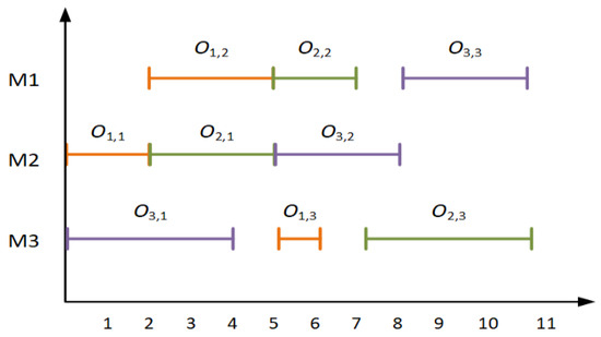
Figure 1.
A feasible 3 3 JSP schedule in Table 1.
3.1. Impact of PM on Operational Completion Time
We assume that machines (i.e., ) have PM activities executed after operations . The feasible schedule with preventive maintenance is shown in Figure 2. A feasible schedule that has executed PM activities. The PM activities are indicated with dark blocks. From the perspective of operation , the other operations can be divided into two sets. The set consisting of is called the associated set of . The set consisting of is called the non-associated set of . For the operations in the associated set, if PM activity occurs before or after one operation, it may cause the delay of . However, the completion time of the operation can only have its delay prevented when a PM activity is executed after the operation . As shown in Figure 2, there are four precedence constrain chains to . In addition, the influence can be delivered to through any chain.
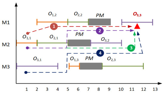
Figure 2.
A feasible schedule that has executed PM activities.
In chain 1, i.e., , the idle time between operations can absorb the impact of PM. The idle time between and can be obtained by . The completion time of operation affected by chain 1, is denoted as .
In chain 2, i.e., , the completion time of the operation , affected by chain 2, is denoted as .
In chain 3, i.e., , the completion time of the operation , affected by chain 3, is denoted as .
In chain 4, i.e., , the completion time of the operation , affected by chain 4, is denoted as .
where , , are all equal to 1, and the rest of the binary variables are 0.
The completion time of the operation caused by PM activities is denoted as
The sequence of PM is determined when the preventive maintenance plan is developed. In addition, the time of PM is often considered a constant. The calculation of PM’s influence on operation completion time is a deterministic problem.
The PM activities have two influences on the initial schedule : ① PM can reduce the possibility of machine failure and increases the stability of schedule; ② PM can reduce the idle time between operations and may increase the makespan of schedule.
3.2. Influence of Machine Failure on Operational Completion Time
The machine breakdowns will lead to the interruption of the processing of the jobs. Since this paper assumes that the jobs continue to be processed after the machines are repaired, it can be considered that the machine breakdowns substantially increase the time the job stays on the machine; at the operational level, it can be regarded as the increase of operation processing time. Assume that these operations (i.e., ) will suffer from breakdowns. The actual schedule is shown in Figure 3, and the breakdowns are indicated with red blocks. Through the same above principle, there are four precedence constrain chains to . The effect can be delivered to through any chain.
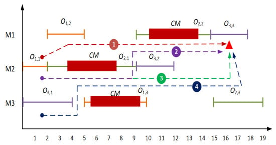
Figure 3.
A feasible schedule that has suffered from machine breakdowns.
The completion time of , affected by chain 1, is denoted as .
The completion time of , affected by chain 2, is denoted as .
The completion time of , affected by chain 3, is denoted as .
The completion time of , affected by chain 4, is denoted as where , and , are all equal to one and the rest of the binary variables are zero.
The completion time of operation caused by machine breakdowns is denoted as . Compared to the PM activities, the CM activities are not only affected by subsequent operations of machine dimension, but are also affected by subsequent operations of job dimension, which will lead to more serious disorder.
Due to stochastic failures, the number and time of machine failures in actual scheduling cannot be obtained before the completion of production. Even though the realized number of breakdowns may be infinite, the complexity of computing increases exponentially with the number of associated operations. For example, the number of operations in the associated operation set of is six. Meanwhile, machine breakdown may occur during the operation . Thus, the number of total scenarios is .
4. Robustness Measure for JSP with Preventive Maintenance
Since the high complexity status and the cost of intensive computation for large problem exists, the exact methods are not suitable for practical application [2]. The Monte Carlo simulation can get accurate results under the condition that the number of simulation times is sufficient, but suffers from a considerable computation burden [3]. Therefore, we propose an analytical approximation method for fast and accurate computing schedule robustness in this section.
4.1. Monte Carlo Simulation
To address stochastic methods regarding RMBs, a set of scenarios randomly generated according to the probability distribution of machine failure are used to simulate RMBs. The scheduling quality robustness can be approximately given by the average of the makespan delay in all scenarios, which can be described as follows:
where denotes the Monte Carlo approximation of the schedule quality robustness, is the number of scenarios, and is the actual makespan of the schedule with breakdowns in the kth simulated scenarios.
The scheduling stability robustness can be approximately given by the average of the total delay time for all operations in all simulated scenarios, which can be described as follows:
where denotes the Monte Carlo approximation of the schedule solution robustness and is the completion time of operation in the schedule .
The precision of measure mainly depends on the number of repetitions of the simulation. However, the computation becomes intensive when N is large [3].
4.2. Analytical Approximation Calculation
Since this paper assumes that the job continues to be processed after the machine is repaired, the machine breakdown essentially increases the residence time of the job on a machine. At the operative level, it can be regarded as an increase in operation processing time. In this paper, machine breakdowns are mapped to the operation level. Then, the breakdown probability of each operation can be computed as
where denotes the age of the machine when operation starts processing, and denotes the age of the machine at the end of the operation .
The expected corrective maintenance time during operation is given by Equation (8).
can be regarded as the expected increase of the processing time of operation by CM.
Machine breakdowns not only affect interrupted operations, but also propagate along with constraints between operations. The influence of failures may be weakened by the idle time between operations or enhanced by superimposed with other failures. Figure 4 shows the influence of RMBs on the single operation and its subsequent operation time arrangement. The expected time spent for the CM activity on the operation is illustrated as a red box. As shown in Figure 4a, the completion time of operation will be delayed when its processing time increases , defined by the delayed completion time . Once the completion time of operation is delayed, the completion time of subsequent operations may be affected. This depends on the idle time between operations, as shown in Figure 4b.The completion time of operation will be delayed . Due to , the completion time of operation will not be delayed. However, if , the completion time of operation will be delayed. Due to , the completion time of partial operations that should be affected may not be changed, which will lead to inaccurate measurement results. Therefore, the expected completion time of operation should be expressed as

Figure 4.
The influence of RMBs on the single operation and its subsequent operation time arrangement. (a) Operation increases expected repair time. (b) The effect of the start time of . (c) The effect of the start time of .
Similarly, the expected completion time of operation is , as shown in Figure 4c.
The effort of computing the expected completion time of operation with the approach presented in Section 3 is not suitable for the practical utility. Therefore, we propose an approximate method for the expected completion time of operation based on failure propagation at the operative level.
Figure 5 shows an example of three jobs and two machines. From the perspective of operation , is the associated operation set of operation . For the operations in the associated operation set, if breakdowns occur in multiple operations, which may occur due to idle time between operations, or enhanced by superposition with other breakdowns, it makes the calculation of operation delay time very complicated. As shown in Figure 5, two chains can affect the completion time of operation .
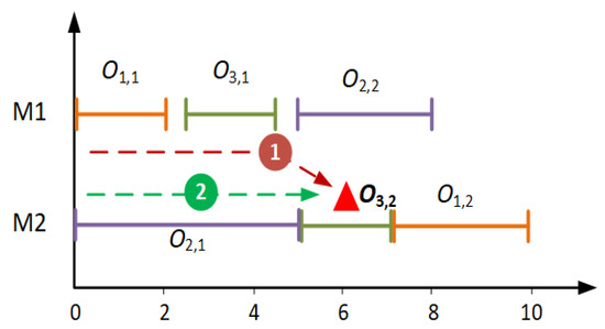
Figure 5.
The Gantt chart for n = 3, m = 2.
In chain 1, i.e., , when the failure occurs in the operation , it may first affect the completion time of operation . As shown in Figure 6b, the expected completion time of is denoted as . The failure will continue to propagate along the chain of constraints, and the operation will be affected. The expected completion time of is . When the failure occurs in the operation , the propagation process is shown in Figure 6c. The expected delay time of affected by RMBs on is denoted as , where . When the failure occurs in the operation , as shown in Figure 6d, the expected delay time of is . The expected completion time of by affected by RMBs on the operation of chain 1 can be denoted as .
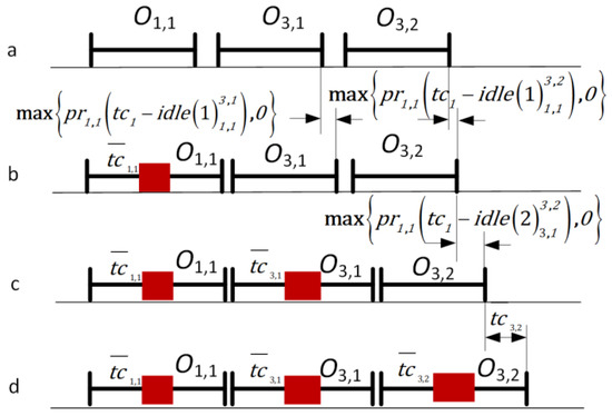
Figure 6.
The calculation of the expected completion time of operation. (a) Process sequence without adding breakdowns (b) The influence of the failure in operation on the completion time of the subsequent operations. (c) The influence of the failure in operation on the completion time of the subsequent operations. (d) The influence of the failure in operation on its own completion time.
The expected completion time of by chain 2 is denoted as . The expected completion time of caused by RMBs is denoted as .
At last, we propose the following surrogate measure to approximate the expected completion time.
The detailed Algorithm1 is shown as follows:
| Algorithm 1 Pseudocode of Approximate estimate |
|
For the robustness evaluation problem of scheduling scheme with operations, since each operation node has at most two successor nodes, the failure impact propagation of each operation only needs to be calculated twice. The total number of calculations is , and its computational complexity is .
4.3. Surrogate Robustness Measures
Three surrogate robustness measures based on slack-time are investigated. First, Leon and Wu [6] applied the average total slack time of all operations to measure the quality robustness of a schedule, as shown in the following:
where indicates total slack time of the operation, .
In contract, Al-Fawzan and Haouari [17] proposed using the sum of free slack times to measure the quality robustness, as shown in the following:
where indicates free slack time of the operation .
Xiong Jian and Xing Lining [15] took the weighted total slack time of all operations as the surrogate robustness measure:
where is the workload of the machine on which operation is processed and is the sum of workloads of all machines.
5. Computational Results
5.1. Experiment Settings
Five measures are available for evaluating the robustness of a schedule: Monte Carlo sampling (MC), the analytical approximation method (AC) proposed by us, and three surrogate robustness measures (). All of these algorithms were coded and implemented in Python on an Intel(R) Core(TM) i5-8350U @CPU 1.60 GHz with RAM 4.00 GB.
To demonstrate the effectiveness of our surrogate measure, this paper presents a variety of comparison SMs that were tested on [31] (ft10, ft20), Davis [32] (la01, la06, la11, la16, la21, la26, la31, la35, la40), Storer, Wu [33] (swv01, swv06, swv11), Taillard [34] (tai01, tai11, tai21, tai31, tai41, tai51), and Yamada and Nakano [35] (yn1). We focus on the performance comparison of different surrogate measures of robustness. The genetic algorithm [36] was used to generate the initial scheduling of all benchmarks. For comparability and ease of implementation reasons, all the parameters of the genetic algorithm are set to the same values. The population size ( and the evolutionary generation are both set to 300, the operation sequence crossover rate was 0.9, and the operation sequence mutation rate was 0.1.
We inserted the PMs to each machine as late as possible, while keeping the constraint that the machine’s age is always smaller than . Then, we obtained the schedule with PMs.
The parameters of instances are set as follows. We set the preventive maintenance time of machine and corrective maintenance; It is assumed that the failure time is subject to a Weibull distribution with shape parameter and scale parameter . Then, we obtain 252 cases.
5.2. Analysis of Different Robustness Measures
In this section, the performance of different robustness measures is analyzed. The Monte Carlo simulation is adopted to approximate the realized schedules. Robustness was indicated by the average value of 5000 samples, as follows:
To verify the accuracy of analytical approximation calculation, and are defined to investigate the difference between the two measures. The smaller the value of , the more accurate the measurement result of the for the solution’s robustness. The same principle applies to .
Table 2 summarizes the experimental results. From Table 2, it is clear that all Mean()s of are close to that of for all tested benchmarks. For the case of , the means of have a maximum value of 7.75%. In addition, all the standard deviations of are less than 4.14%. Similar results can also be found for , where the values are less than 2.27%. The standard deviations of is within [0.29%, 1.42%]. The experimental results show that can be valid substitution for ,. Table 2 also provides the results of CPU time in seconds for measuring the robustness based on . It shows that the mean CPU time based on is much smaller than that based on ; the time ratio between and is within [0.35%, 0.74%]. Meanwhile, as the machine failure rate and CM time increase, the computing time required by increases more significantly than that required by . Therefore, has higher computing efficiency than .

Table 2.
Evaluate the performance of .
The distributions of are available in Figure 7a by a quartile graph. Figure 7a shows that the largest of all tested benchmark problems is below 14.40%. In addition, it can also be found that will decrease significantly with the reduction of failure probability. Figure 7b shows that is stable, but with the increase of , the fluctuation of becomes larger. The experimental results show that the performance of is better when the failure probability and CM time are small.
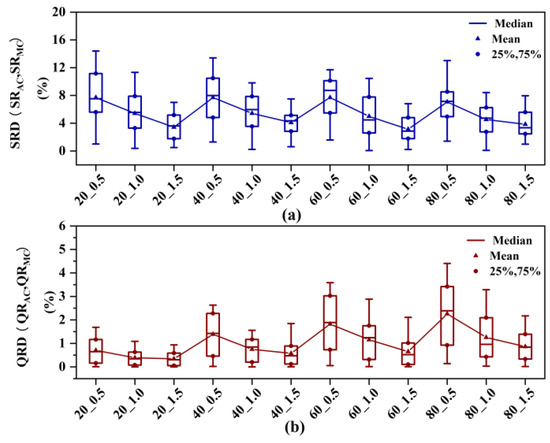
Figure 7.
Quartile graph of SRD, QRD for every benchmark problem. (a) Quartile graph of SRD at different fault levels. (b) Quartile graph of QRD at different fault levels.
5.3. Performance Comparison with Other Surrogate Robustness Measures
To efficiently approximate the robustness of a schedule, a measure must perform a strong linear correlation to exact robustness. A correlation study is performed in this section. Since the robustness of the schedule cannot be calculated precisely, the correction study will be performed using a Monte Carlo simulation as an approximation. The value is expected to predict the robustness of the schedule. A measure with a higher value is expected to better predict schedule robustness.
As shown in Table 3, all significance values of are smaller than 0.001, whereas most significance values of , and are larger than 0.001. This indicates that has a more significant linear correlation with the solution robustness. In addition, all values of are quite close to one and significantly larger than the others. This implies that can more efficiently approximate the schedule stability than the other measures.

Table 3.
Solution robustness correlation analysis.
Figure 8a clearly shows that has the lowest linear correlation with , and that and have similar linear correction with .
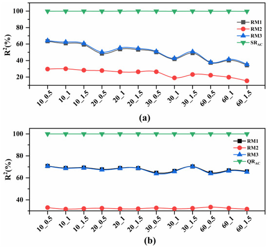
Figure 8.
Comparison of values at different fault levels. (a) Compare of values in solution robustness. (b) Compare of values in quality robustness.
As shown in Table 4, the significance values of and other measures are all maintained at a tiny value. All values of are almost close to 1.0 and larger than that of the others. This indicates that can approximate the schedule robustness more efficiently than the other measures.

Table 4.
Quality robustness correlation analysis.
Figure 8b shows that the also has minimum linear correlation with . The values of and are in the range of [0.6, 0.85] and fluctuate with the change of failure parameters. This indicates that RM2 and can partially approximate the quality robustness of schedule.
To summarize, the three surrogate robustness measures can only perform well in the case of a very high level of RMB, while can adapt to various levels of RMB conditions.
5.4. Comparison between the Integrated PM Schedule and Non-PM Schedule
The performance difference between the integrated PM schedule and the non-PM schedule is demonstrated. Three evaluation criteria are defined to investigate the difference between the two schedules and in schedule performance. indicates the solution robustness improvement ratio of to , as shown in Equation (18). If is greater than zero, it indicates that the solution robustness of is better than , and vice versa. is defined to investigate the performance improvement ratio of to , as shown in Equation (19). If is greater than zero, it indicates that has advantages to in scheduling performance, and vice versa. indicates the quality robustness improvement radio of to . If is greater than zero, it indicates that the has advantages to in quality robustness.
In Section 3.1, we pointed out that PM activities can increase scheduling stability and may also reduce scheduling performance. Excellent PM insertion strategies can enhance scheduling stability and performance at the same time. As shown in Table 5, most values are greater than zero, which indicates that the scheduling stability improved after PM activities. However, values varied greatly under different fault settings. In the case of (20,1.0), (20,1.5), (40,1.0), (40,1.5), and (60,1.5), the values of are less than 0, which indicates that scheduling performance after inserting PM activities is worse than that of initial schedule under the condition of low failure probability or little CM time. For , the experimental data have the same characteristics as values. One possible reason for this case is that the QR value is part of SR and is more sensitive to changes in fault parameters.

Table 5.
Relative difference between and .
To show the above analysis more clearly, the experimental data are also shown in Figure 9. We have a few key findings. Figure 9a shows the quartile graph of SRIR. When is the same, the SRIR values increase with the increase of CM time. This indicates that, when the machine failure probability is constant, SRIR values are positively correlated with CM time. It also shows that it is more effective to insert PM activities when the CM time is too long. At the same time, when the CM time is fixed, the SRIR values decrease gradually with the reduction of fault probability, indicating that the improvement effect on the stability of the scheduling scheme is limited when the fault probability is small.
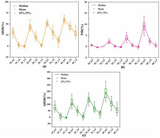
Figure 9.
Quartile graph of , and for every benchmark problem. (a) Quartile graph of at different fault levels. (b) Quartile graph of at different fault levels. (c) Quartile graph of at different fault levels.
Figure 9b shows the quartile graph of PIR. Figure 9b shows the same trend as Figure 9a, but some PIR values are less than 0 when the fault probability is low, and the CM time is short. The reason for this result is that the delay in the initial scheduling makespan caused by the failure is less than the impact of PM activities.
Figure 9c shows that the quartile graph of QRIR and its variation trend are the same as SRIR. We also can find that the QRIR of the schedule that inserts PM activities under the condition of high machine failure probability and large CM time is better.
6. Conclusions
In this paper, we studied the problem of evaluating two categories of robustness for the reliable schedule to be obtained by inserting PM activities. We transform the problem into the calculation of the expected completion time of operation and derive an accurate analytical expression. Due to the high burden of practical calculation, we also proposed an analytical approximation based on the internal relationships among the scheduling structure, the number and sequence of PM activities, the probability and downtime of failures, and the completion time of operation. Compared with Monte Carlo simulations, the proposed method has almost the same accuracy and lower computation burden. Through a comparison with the state-of-the-art surrogate robustness measures, the experimental results show that the proposed measure is far superior to the other three surrogate measures in all cases. Additional experiments were carried out to demonstrate the importance of PM activities, especially in the case of high failure probability and long CM time.
Several lines of future work might be explored. First, machine failure probability and repair time are considered to be known, but this information is often unknown in actual production; the robustness evaluation model can be established from the perspective of fuzzy theory or data mining. Additionally, more uncertain factors in production (such as uncertain processing time, uncertain job arrival time, and rework) can be incorporated into the evaluation model. Finally, based on the robustness evaluation model, we hope to further propose a new algorithm to optimize the insertion order of PM activities to significantly improve the stability and performance of scheduling.
Author Contributions
For Conceptualization, Z.B.; methodology, Z.B.; software, Z.B.; validation, Z.B.; writing—original draft preparation, Z.B.; writing—review and editing, Y.Y. All authors have read and agreed to the published version of the manuscript.
Funding
This research was funded by the National Natural Science Foundation of China [grant number 71961029] and the Key Research and Development project of Xinjiang Uygur Autonomous Region [grant number 2020B02013].
Institutional Review Board Statement
Not applicable. (This study does not involve humans or animals).
Informed Consent Statement
Not applicable.
Data Availability Statement
The data that support the findings of this study are openly available at http://optimizizer.com/jobshop.php (accessed on 1 January 2016).
Conflicts of Interest
The authors declare no conflict of interest.
References
- Von Hoyningen-Huene, W.; Kiesmueller, G.P. Evaluation of the expected makespan of a set of non-resumable jobs on parallel machines with stochastic failures. Eur. J. Oper. Res. 2015, 240, 439–446. [Google Scholar] [CrossRef]
- Jin, Y.; Branke, H. Evolutionary optimization in uncertain environments—A survey. IEEE Trans. Evol. Comput. 2005, 9, 303–317. [Google Scholar] [CrossRef]
- Wu, Z.G.; Sun, S.D.; Xiao, S.C. Risk measure of job shop scheduling with random machine breakdowns. Comput. Oper. Res. 2018, 99, 1–12. [Google Scholar] [CrossRef]
- Ouelhadj, D.; Petrovic, S. A survey of dynamic scheduling in manufacturing systems. J. Sched. 2009, 12, 417–431. [Google Scholar] [CrossRef]
- Herroelen, W.; Leus, R. Project scheduling under uncertainty: Survey and research potentials. Eur. J. Oper. Res. 2005, 165, 289–306. [Google Scholar] [CrossRef]
- Leon, V.J.; Wu, S.D.; Storer, R.H. Robustness measures and robust scheduling for job shops. IIE Trans. 1994, 26, 32–43. [Google Scholar] [CrossRef]
- Mehta, S.V.; Uzsoy, R.M. Predictable scheduling of a job shop subject to breakdowns. IEEE Trans. Robot. Autom. 1998, 14, 365–378. [Google Scholar] [CrossRef]
- O’Donovan, R.; Uzsoy, R.; McKay, K.N. Predictable scheduling of a single machine with breakdowns and sensitive jobs. Int. J. Prod. Res. 1999, 37, 4217–4233. [Google Scholar] [CrossRef]
- Goren, S.; Sabuncuoglu, I. Robustness and stability measures for scheduling: Single-machine environment. IIE Trans. 2008, 40, 66–83. [Google Scholar] [CrossRef]
- Al-Hinai, N.; ElMekkawy, T.Y. Robust and stable flexible job shop scheduling with random machine breakdowns using a hybrid genetic algorithm. Int. J. Prod. Econ. 2011, 132, 279–291. [Google Scholar] [CrossRef]
- Zandieh, M.; Gholami, M. An immune algorithm for scheduling a hybrid flow shop with sequence-dependent setup times and machines with random breakdowns. Int. J. Prod. Res. 2009, 47, 6999–7027. [Google Scholar] [CrossRef]
- Paprocka, I.; Skolud, B. A hybrid multi-objective immune algorithm for predictive and reactive scheduling. J. Sched. 2017, 20, 165–182. [Google Scholar] [CrossRef]
- Ahmadi, E.; Zandieh, M.; Farrokh, M.; Emami, S.M. A multi objective optimization approach for flexible job shop scheduling problem under random machine breakdown by evolutionary algorithms. Comput. Oper. Res. 2016, 73, 56–66. [Google Scholar] [CrossRef]
- Liu, L.; Gu, H.Y.; Xi, Y.G. Robust and stable scheduling of a single machine with random machine breakdowns. Int. J. Adv. Manuf. Technol. 2007, 31, 645–654. [Google Scholar] [CrossRef]
- Xiong, J.; Xing, L.; Chen, Y. Robust scheduling for multi-objective flexible job-shop problems with random machine breakdowns. Int. J. Prod. Econ. 2013, 141, 112–126. [Google Scholar] [CrossRef]
- Hazir, O.; Haouari, M.; Erel, E. Robust scheduling and robustness measures for the discrete time/cost trade-off problem. Eur. J. Oper. Res. 2010, 207, 633–643. [Google Scholar] [CrossRef]
- Al-Fawzan, M.A.; Haouari, M. A bi-objective model for robust resource-constrained project scheduling. Int. J. Prod. Econ. 2005, 96, 175–187. [Google Scholar] [CrossRef]
- Kobylanski, P.; Kuchta, D. A note on the paper by M. A. Al-Fawzan and M. Haouari about a bi-objective problem for robust resource-constrained project scheduling. Int. J. Prod. Econ. 2007, 107, 496–501. [Google Scholar] [CrossRef]
- Zhang, G.; Lu, X.; Liu, X.; Zhang, L.; Wei, S.; Zhang, W. An effective two-stage algorithm based on convolutional neural network for the bi-objective flexible job shop scheduling problem with machine breakdown. Expert Syst. Appl. 2022, 203, 117460. [Google Scholar] [CrossRef]
- Xiao, S.; Sun, S.; Jin, J. Surrogate Measures for the Robust Scheduling of Stochastic Job Shop Scheduling Problems. Energies 2017, 10, 26. [Google Scholar] [CrossRef]
- Chansombat, S.; Pongcharoen, P.; Hicks, C. A mixed-integer linear programming model for integrated production and preventive maintenance scheduling in the capital goods industry. Int. J. Prod. Res. 2019, 57, 61–82. [Google Scholar] [CrossRef]
- Khatami, M.; Zegordi, S.H. Coordinative production and maintenance scheduling problem with flexible maintenance time intervals. J. Intell. Manuf. 2017, 28, 857–867. [Google Scholar] [CrossRef]
- Rahmati, S.H.A.; Ahmadi, A.; Karimi, B. Multi-objective evolutionary simulation based optimization mechanism for a novel stochastic reliability centered maintenance problem. Swarm Evol. Comput. 2018, 40, 255–271. [Google Scholar] [CrossRef]
- Avalos-Rosales, O.; Angel-Bello, F.; Álvarez, A.; Cardona-Valdés, Y. Including preventive maintenance activities in an unrelated parallel machine environment with dependent setup times. Comput. Ind. Eng. 2018, 123, 364–377. [Google Scholar] [CrossRef]
- Cui, W.; Lu, Z.; Li, C.; Han, X. A proactive approach to solve integrated production scheduling and maintenance planning problem in flow shops. Comput. Ind. Eng. 2018, 115, 342–353. [Google Scholar] [CrossRef]
- Feng, H.X.; Xi, L.F.; Xiao, L.; Xia, T.B.; Pan, E.S. Imperfect preventive maintenance optimization for flexible flowshop manufacturing cells considering sequence-dependent group scheduling. Reliab. Eng. Syst. Saf. 2018, 176, 218–229. [Google Scholar] [CrossRef]
- Torres, P.J.R.; Mercado, E.I.S.; Santiago, O.L.; Rifon, L.A. Modeling preventive maintenance of manufacturing processes with probabilistic Boolean networks with interventions. J. Intell. Manuf. 2018, 29, 1941–1952. [Google Scholar] [CrossRef]
- Cui, W.-W.; Lu, Z.; Pan, E. Integrated production scheduling and maintenance policy for robustness in a single machine. Comput. Oper. Res. 2014, 47, 81–91. [Google Scholar] [CrossRef]
- Sevaux, M.; Sörensen, K. A genetic algorithm for robust schedules in a one-machine environment with ready times and due dates. Q. J. Belg. Fr. Ital. Oper. Res. Soc. 2004, 2, 129–147. [Google Scholar] [CrossRef]
- Abumaizar, R.J.; Svestka, J.A. Rescheduling job shops under random disruptions. Int. J. Prod. Res. 1997, 35, 2065–2082. [Google Scholar] [CrossRef]
- Muth, J.F.; Thompson, G.L.; Winters, P.R. Industrial Scheduling; PWS Pub. Co.: Boston, MA, USA, 1997. [Google Scholar]
- Davis, L. Job Shop Scheduling with Genetic Algorithms; Psychology Press: London, UK, 1985; pp. 136–140. [Google Scholar]
- Storer, R.; Wu, S.; Vaccari, R. New Search Spaces for Sequencing Problems with Application to Job Shop Scheduling. Manag. Sci. 1992, 38, 1495–1509. [Google Scholar] [CrossRef]
- Taillard, E. Benchmarks for basic scheduling problems. Eur. J. Oper. Res. 1993, 64, 278–285. [Google Scholar] [CrossRef]
- Yamada, T.; Nakano, R. A Genetic Algorithm Applicable to Large-Scale Job-Shop Problems. PPSN 1992, 2, 283–292. [Google Scholar]
- Della Croce, F.; Tadei, R.; Volta, G. A genetic algorithm for the job shop problem. Comput. Oper. Res. 1995, 22, 15–24. [Google Scholar] [CrossRef]
Disclaimer/Publisher’s Note: The statements, opinions and data contained in all publications are solely those of the individual author(s) and contributor(s) and not of MDPI and/or the editor(s). MDPI and/or the editor(s) disclaim responsibility for any injury to people or property resulting from any ideas, methods, instructions or products referred to in the content. |
© 2023 by the authors. Licensee MDPI, Basel, Switzerland. This article is an open access article distributed under the terms and conditions of the Creative Commons Attribution (CC BY) license (https://creativecommons.org/licenses/by/4.0/).