
The Stationary Thermal Field in a Multilayer Elliptic Cylinder
Abstract
:1. Introduction
2. Physical and Mathematical Models
3. Calculation Example—Electric Conductor with Double Insulation
a3 = 0.0199005 m, λ1 = 180 W/(mK), λ2 = 0.17 W/(mK), λ3 = 0.16 W/(mK), α = 14.9 W/(m2K), ρ(70 °C) = 3.39592 × 10⁻⁸ Ωm, Tmax = 70 °C, Ta = 25 °C, ks = 1.02, kn = 1.02.
4. Verification of the Results
5. Conclusions
- An analytical–numerical method for the determination of the thermal field in a multilayer elliptical system was presented in the paper. An example of application is the analysis of the thermal field in a double-insulation conductor. The eigenfunctions (6) were computed analytically by the superposition of the general and particular solutions of the Poisson Equation (2) [29] and by the variable-separation method. In turn, the coefficients of the eigenfunctions were computed by the iterative solution of the system of Equations (22) and (23) after numerical computation of the integrals in (24)–(30).
- Compared to the numerical methods, the technique presented in the article has the following advantages:
- -
- no need for area discretization;
- -
- no need for area discretization;
- -
- the possibility of calculating field values at any point in the system and not only at grid nodes;
- -
- Formulas (8), (15) and (16) support the physical interpretation and discussion of the influence of individual parameters. Moreover, they facilitate the determination of scaling laws and the fast estimation of the field at selected points;
- -
- Formulas (8), (15) and (16) enable easy calculation of the sum of series with the necessary limitation of the number of summed terms (due to the calculation time).
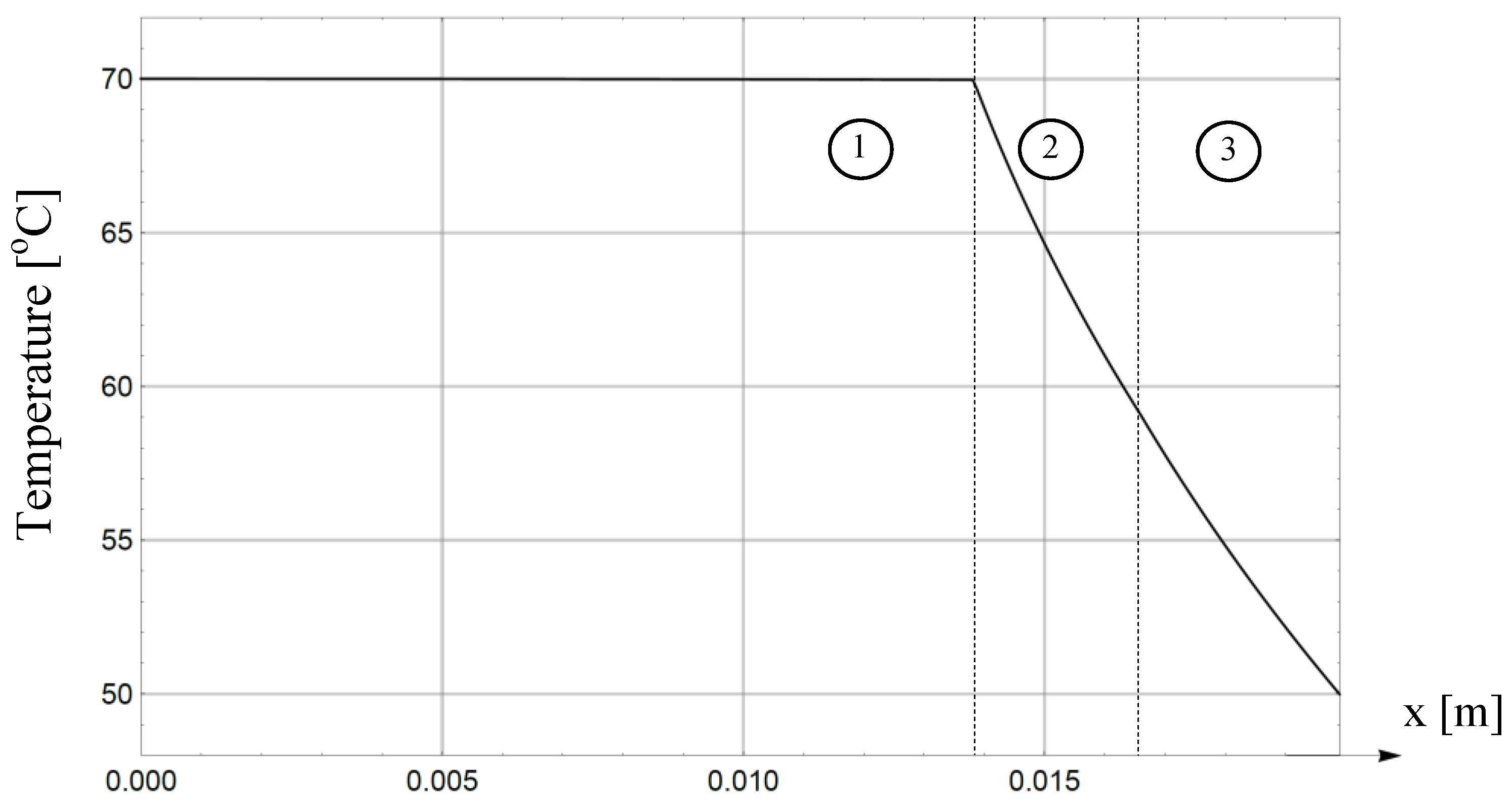
- The thermal field in the central part of the system (0 ≤ η ≤ η1) is almost uniform. This is observed both in the conductor core (Figure 2, Figure 3 and Figure 4) and in the test model (Figure 5 and Figure 6). The maximum temperature drop in the conductor core is negligible: T1(η = 0, ψ = π/2) − T1(η = η1, ψ = 0) = 0.034 °C. In the test system, the respective temperature drop is 0.033 °C. The uniformity of the field is justified by a very large thermal conductivity in the central part of the system (λ1 = 180 W/(mK)).
- Clear temperature drops occur in regions of lower heat conductivity, compared to the central part (λ2 << λ1, λ3 << λ1). The drop increases with the increase in insulation thickness. For example, for the conductor, the following occurs: ({b3 − b1 ≈ 8.99 mm > a3 − a1 ≈ 6.08 mm} => {T1(η = η1, ψ = π/2) − T3(η = η3, ψ = π/2) = 22.09 °C > T1(η = η1,ψ = 0) − T3(η = η3, ψ = 0)= 19.99 °C})—Figure 1. The above is due to the increase in the thermal resistance of two layers of insulation with their total thickness and to thermal Ohm’s law.
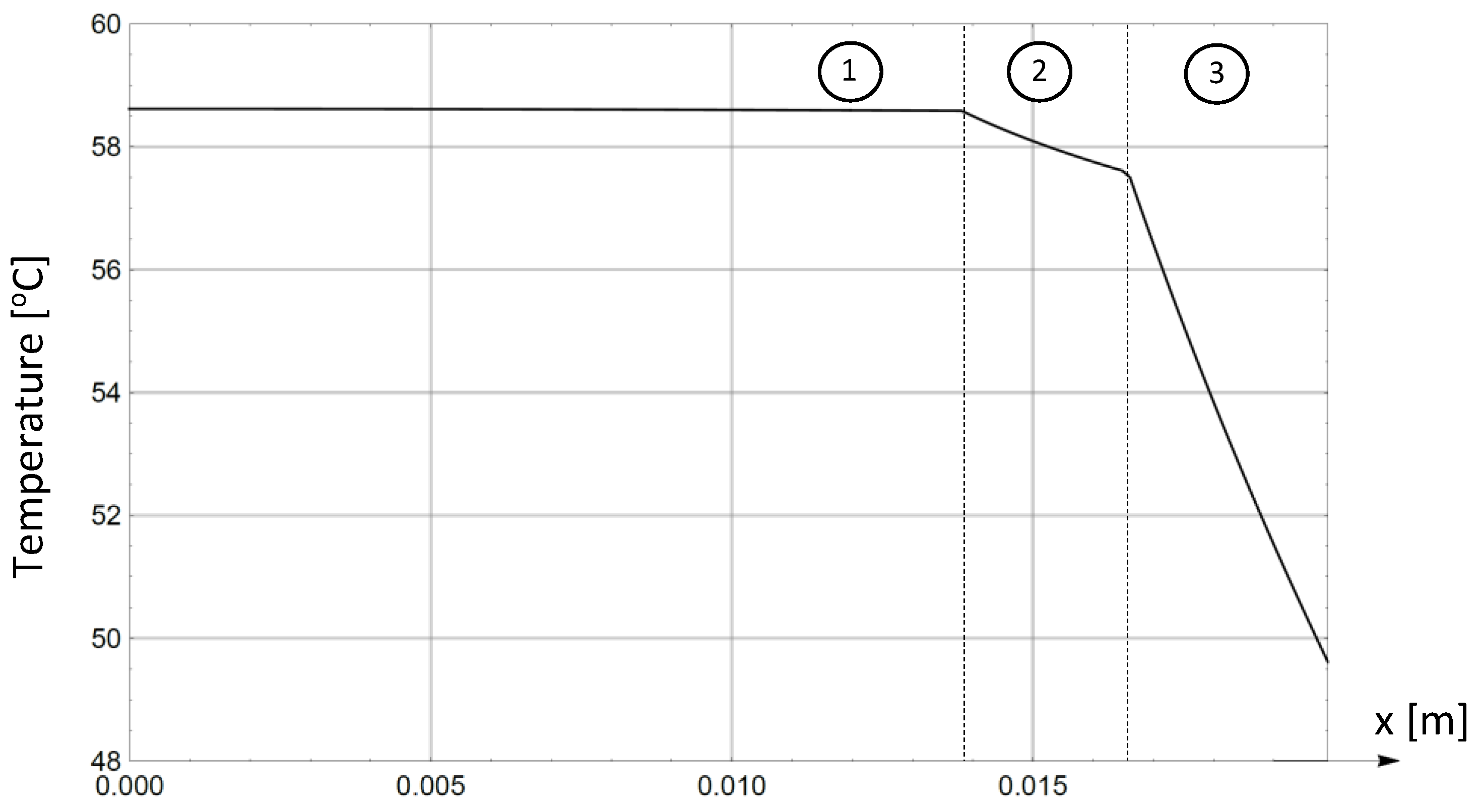
- The increase in the thermal conductivity of the middle layer λ2 (e.g., tenfold) substantially changes the thermal field distribution. For the conductor, the temperature drop in the double insulation is almost linear (Figure 2 and Figure 3). In the test model, the temperature drop is continuous by sections (Figure 5 and Figure 6). In addition, the maximum temperature decreases from 70.01 °C (Figure 2 and Figure 3) to 58.62 °C (Figure 5 and Figure 6). This is due to better heat dissipation with the increase in λ2.
- On the system’s outer perimeter (η = η3), the temperature decreases from T3(η = η3, ψ = 0) = 49.99 °C to T3(η = η3, ψ = π/2) = 47.91 °C for the conductor, and from 49.61 °C to 48.22 °C for the test system. The above proves that the layer boundaries (ellipses η1, η2, η3) are not isotherms. This is due to the variable distance of the points on the ellipses η1, η2, η3 from the system’s center (η = 0, ψ = π/2).
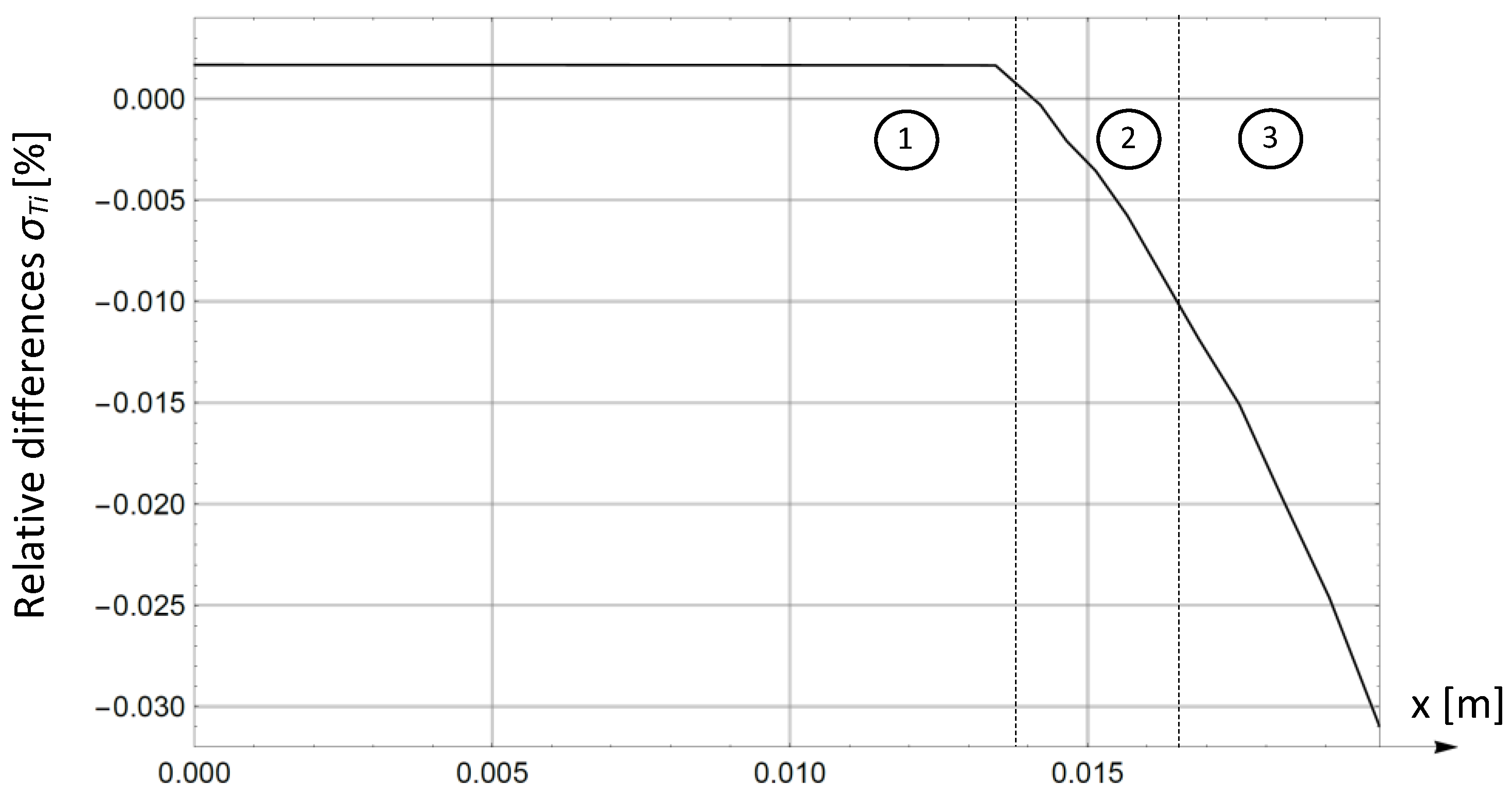
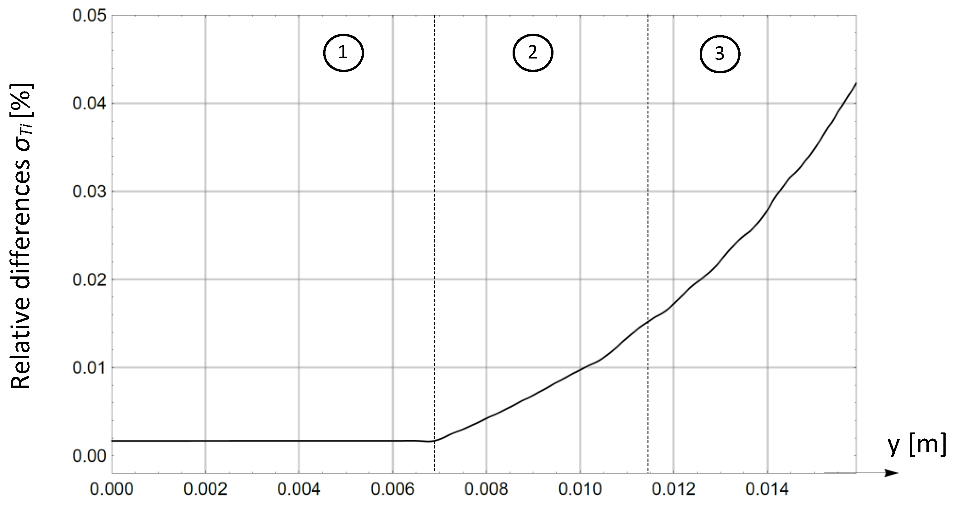
- Figure 7 and Figure 8 show that the relative differences (34) between the temperature distributions (as calculated, respectively, by the method presented in the paper and numerical method) are very small. Therefore, the above-mentioned methods give very similar results. The module of difference (34) is the smallest in the region with a uniform temperature field (0 ≤ η ≤ η1). This is justified by the greater accuracy of the finite element method in regions with a small field gradient.
- The method presented in the paper may find application in various fields of technology. An example of this is dielectric heating of an elliptical cylinder composed of dielectric layers. Using the method described in the paper, two important parameters can be determined: the maximum temperature and the gradient of its decrease. Exceeding these parameters can result in the loss of desired properties of the dielectric charge or even its destruction. Another application is the analysis of the electrostatic field in layered elliptical systems.
Author Contributions
Funding
Institutional Review Board Statement
Informed Consent Statement
Data Availability Statement
Conflicts of Interest
List of Symbols
| A0, B0, C0, D0, E0 | unknown constants in relationships (8)–(10), |
| Ai, Bi, Ci, Di | constants in the relationship (6), |
| An, Fn, Gn, Pn, Qn | unknown coefficients in relationships (8)–(10), |
| Ani, Bni, Cni, Dni | coefficients in the relationship (6), |
| a1,a2 …aN | successive semi-major axes of ellipses, |
| b1,b2 …bN | successive semi-minor axes of ellipses, |
| c | x-coordinate of the focus, |
| f(n), g(n), p(n), q(n) | functions described by Formulas (17)–(20), |
| gi | heat source with efficiency for i = 1,2, …N, |
| h(m, n), r(n) | functions described by Formulas (30) and (31), |
| I1(..,..), I2(..), I3(n), I4 | integrals described by relationships (24)–(29), |
| |I| | root-mean square current, |
| Icr | current-carrying capacity (or ampacity), |
| kn | skin effect coefficient, |
| ks | elongation coefficient, |
| l | length of the conductor, |
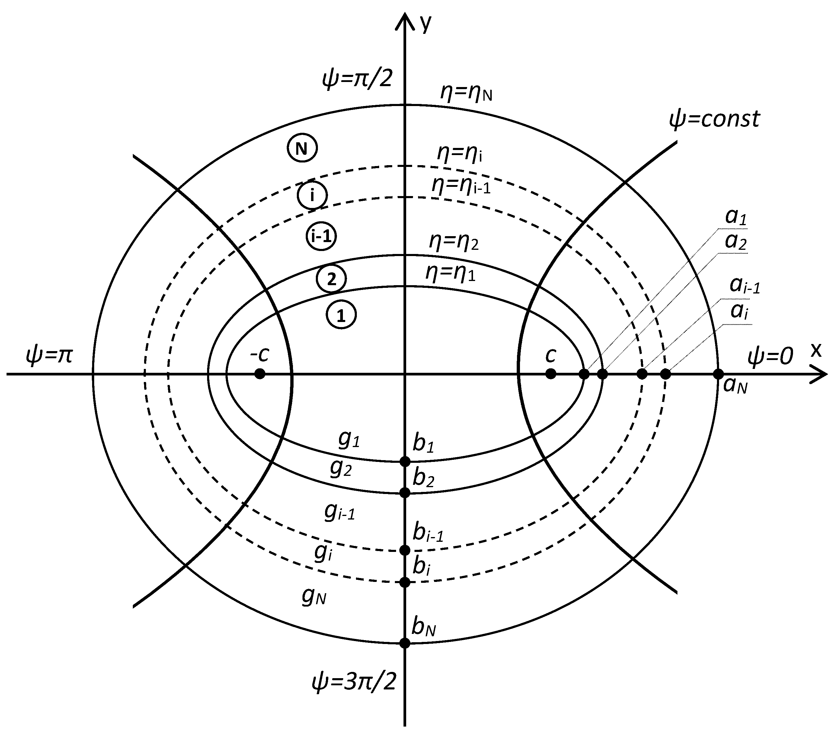
| N | number of the given ellipse (Figure 1), |
| n | summation index, |
| P1 | power of heat losses, |
| RAC | AC resistance, |
| RDC | DC resistance, |
| heat flux vector, | |
| S1 | sum of the cross-sections helically stranded wires in the core, |
| Ta | ambient temperature, |
| Tmax | maximum long-term operating temperature, |
| Ti(..,..) | two-dimensional stationary distribution of the thermal field for i = 1,2, …N, |
| temperature distribution in the i-th zone calculated by the finite element method, | |
| V1 | volume of conductor length, |
| α | heat transfer coefficient, |
| δTi | relative differences defined by the relationship (34), |
| ηi | ellipses perimeters for i = 1,2, …N, |
| (η, ψ) | elliptical-cylindrical coordinates, |
| λi | thermal conductivity of the i-th layer, |
| νi(..,..) | temperature increment in the i-th layer, |
| ρ(Tmax) | resistivity of the conductor at Tmax temperature, |
References
- COMSOL Multiphysics. Documentation for COMSOL; Release 4.3; COMSOL, Inc.: Stockholm, Sweden, 2013. [Google Scholar]
- Manuals for NISA v.16, NISA Suite of FEA Software (CD-ROM); Cranes Software Inc.: Troy, MI, USA, 2008.
- Hahn, D.W.; Ozisik, M.N. Heat Conduction; John Wiley & Sons: Hoboken, NJ, USA, 2012. [Google Scholar]
- Tittle, C.W.; Robinson, V.L. Analytical Solution of Conduction Problems in Composite Media; ASME Paper No. 65-WA/HT-52; ASME: New York, NY, USA, 1965. [Google Scholar]
- Tittle, C.W. Boundary value problems in composite media: Quasi-orthogonal functions. J. Appl. Phys. 1965, 36, 1486–1488. [Google Scholar] [CrossRef]
- Mikhailov, M.D.; Ozisik, M.N. Unified Analysis and Solutions of Heat and Mass Diffusion; Dover Publications: Mineola, NY, USA, 1994. [Google Scholar]
- Ozisik, M.N. Boundary Value Problems of Heat Conductions; Dover Publications: Mineola, NY, USA, 1989. [Google Scholar]
- Carslaw, H.S.; Jaeger, J.C. Conduction of Heat in Solids; Oxford University Press: London, UK, 1959. [Google Scholar]
- Arpaci, V.S. Conduction Heat Transfer; Addison-Wesley: Reading, MA, USA, 1966. [Google Scholar]
- Luikov, A.V. Analytical Heat Diffusion Theory; Academic Press: New York, NY, USA, 1966. [Google Scholar]
- Crank, J. The Mathematics of Diffusion; Clarendon Press: Oxford, UK, 1975. [Google Scholar]
- Haji-Sheikh, A.; Mashena, M. Integral solution of diffusion equation; part 1-general solution. J. Heat Transfer. 1987, 109, 551–556. [Google Scholar] [CrossRef]
- Mikhailov, M.D.; Ozisik, M.N. Unified solutions of heat diffusion in a finite region involving a surface film of finite heat capacity. Int. J. Heat Mass Transf. 1985, 28, 1039–1045. [Google Scholar] [CrossRef]
- Haji-Sheikh, A.; Beck, J.V. Green’s function partitioning in Galerkin-based integral solution of the diffusion equation. J. Heat Transfer. 1990, 112, 28–34. [Google Scholar] [CrossRef]
- Wu, X.; Shi, J.; Lei, H.; Li, Y.; Okine, L. Analytical solutions of transient heat conduction in multilayered slabs and application to thermal analysis of landfills. J. Cent. South Univ. 2019, 26, 3175–3187. [Google Scholar] [CrossRef]
- Eremin, A.V.; Stefanyuk, E.F.; Kurganova, O.Y.; Tkachev, V.K.; Skvorstova, M. A generalized function in heat conductivity problems for multilayer structures with heat sources. J. Mach. Manuf. Reliab. 2018, 47, 249–255. [Google Scholar] [CrossRef]
- Monte, d.F. An analytical approach to the unsteady heat conduction processes in one-dimensional composite media. Int. J. Heat Mass Transf. 2002, 45, 1333–1343. [Google Scholar] [CrossRef]
- Tatsii, R.M.; Pazen, O.Y. Direct (classical) method of calculation of the temperature field in a hollow multilayer cylinder. J. Eng. Phys. Thermophys. 2018, 91, 1373–1384. [Google Scholar] [CrossRef]
- Monte, d.F. Unsteady heat conduction in two-diemensional two slab-shaped regions. Exact closed-form solution and result. Int. J. Heat Mass Transf. 2003, 1455–1469. [Google Scholar] [CrossRef]
- Singh, S.; Jain, P.K.; Rizwan-uddin. Analytical solution to transient heat conduction in polar coordinates with multiple layers in radial direction. Int J Therm Sci. 2008, 47, 261–273. [Google Scholar] [CrossRef]
- Jain, P.K.; Singh, S. Rizwan-uddin, Analytical solution to transient asymmetric heat condution in a multilayers annulus. J. Heat Transfer. 2009, 131, 1–7. [Google Scholar] [CrossRef]
- Jain, P.K.; Singh, S.; Rizwan-uddin. An exact analytical solution for two-diemsional, unsteady, multilayer heat conduction is spherical coordinates. Int. J. Heat Transfer. 2010, 53, 2133–2142. [Google Scholar] [CrossRef]
- Norouzi, M.; Delouei, A.; Seilsepour, M. A general exact solution for heat conduction in multilayer spherical composite laminates. Compos. Struct. 2013, 106, 288–295. [Google Scholar] [CrossRef]
- Dalir, N.; Nourazar, S.S. Analytical solution of the problem on the tree-dimensional transient heat conduction in a multilayer cylinder. J. Eng. Phys. Thermophys. 2014, 87, 89–97. [Google Scholar] [CrossRef]
- Haji-Sheikh, A.; Beck, J.V. Temperature solution in multi-dimensional mutli-layer bodies. Int. J. Heat Mass Transf. 2002, 45, 1865–1877. [Google Scholar] [CrossRef]
- Benmerkhi, M.; Afrid, M.; Groulx, D. Thermally developing forced convection in a metal foam-filled elliptic annulus. Int. J. Heat Mass Transf. 2016, 97, 253–269. [Google Scholar] [CrossRef]
- Ragueb, H.; Mansouri, K. An analytical study of the periodic laminar forced convection of non-Newtonian nanofuid flow inside an alliptical duct. Int. J. Heat Mass Transf. 2018, 127, 469–483. [Google Scholar] [CrossRef]
- Mahfouz, F.M. Heat conduction within an elliptic annulus heated at either CWT or CHF. Appl. Math. Comput. 2015, 266, 357–368. [Google Scholar] [CrossRef]
- Moon, P.; Spencer, D.E. Field Theory Handbook; Springer: Berlin, Germany, 1988. [Google Scholar]
- Wang, P.; Zhao, M.; Du, X. Analytical solution and simplified formula for earthquake induced hydrodynamic pressure on elliptical hollow cylinder ina water. Ocean Eng. 2018, 148, 149–160. [Google Scholar] [CrossRef]
- Kukla, S. Green’s function for vibration problems of an elliptical membrane. Sci. Res. Inst. Math. Comput. Sci. 2011, 10, 129–134. [Google Scholar]
- Ozisik, M.N. Heat Conduction; John Wiley & Sons: New York, NY, USA, 1992. [Google Scholar]
- Cole, K.D.; Beck, J.V.; Haji-Sheikh, A.; Litkouhi, B. Heat Conduction Using Green’s Functions; CRC Press: Boca Raton, FL, USA, 2011. [Google Scholar]
- Incropera, F.; De Witt, D.; Bergman, T.; Lavine, A. Introduction to Heat Transfer; John Wiley and Sons: New York, NY, USA, 2007. [Google Scholar]
- Nield, D.A.; Bejan, A. Convection in porous media; Springer: New York, NY, USA, 2014. [Google Scholar]
- Raza, J.; Mebarek-oudina, F.; Ali Lund, L. The flow of magnetised convective Casson liquid via a porous channel with shrinking and stationary walls. Pramana-J. Phys. 2022, 96, 229. [Google Scholar] [CrossRef]
- Hassan, M.; Mebarek-oudina, F.; Faisal, A.; Ghavar, A.; Ismail, A.I. Thermal energy and mass transport of shear thinning fluid under effects of low to high shear rate viscosity. Int. J. Thermofluids 2022, 15, 100176. [Google Scholar] [CrossRef]
- Anders, G.J. Rating of Electric Power Cables: Ampacity Computations for Transmission, Distribution and Industrial Application; McGraw-Hill Professional: New York, NY, USA, 1997. [Google Scholar]
- Wolfram Research Inc. Mathematica; Wolfram Research Inc.: Champaign, IL, USA, 2020. [Google Scholar]
- Huebner, K.H.; Dewhirst, D.L.; Smith, D.E.; Byrom, T.G. The Finite Element Method for Engineers; John Wiley and Sons: New York, NY, USA, 2001. [Google Scholar]


Disclaimer/Publisher’s Note: The statements, opinions and data contained in all publications are solely those of the individual author(s) and contributor(s) and not of MDPI and/or the editor(s). MDPI and/or the editor(s) disclaim responsibility for any injury to people or property resulting from any ideas, methods, instructions or products referred to in the content. |
© 2023 by the authors. Licensee MDPI, Basel, Switzerland. This article is an open access article distributed under the terms and conditions of the Creative Commons Attribution (CC BY) license (https://creativecommons.org/licenses/by/4.0/).
Share and Cite
Gołębiowski, J.; Zaręba, M. The Stationary Thermal Field in a Multilayer Elliptic Cylinder. Appl. Sci. 2023, 13, 2354. https://doi.org/10.3390/app13042354
Gołębiowski J, Zaręba M. The Stationary Thermal Field in a Multilayer Elliptic Cylinder. Applied Sciences. 2023; 13(4):2354. https://doi.org/10.3390/app13042354
Chicago/Turabian StyleGołębiowski, Jerzy, and Marek Zaręba. 2023. "The Stationary Thermal Field in a Multilayer Elliptic Cylinder" Applied Sciences 13, no. 4: 2354. https://doi.org/10.3390/app13042354