Abstract
This paper proposes a hybrid evaluation method to assess the prediction models for airport passenger throughput (APT). By analyzing two hundred three airports in China, five types of models are evaluated to study the applicability to different airports with various airport passenger throughput and developing conditions. The models were fitted using the historical data before 2014 and were verified by using the data from 2015–2019. The evaluating results show that the models employed for evaluating perform well in general except that there are insufficient historical data for modelling, or the APT of the airports changes abruptly owing to expansion, relocation or other kinds of external forces such as earthquakes. The more the APT of an airport is, the more suitable the models are for the airport. Particularly, there is no direct relation between the complexity and the predicting accuracy of the models. If the parameters of the models are properly set, time series models, causal models, market share methods and analogy-based methods can be utilized to predict the APT of 88% of studied airports effectively.
1. Introduction
An accurately predicting result of passenger throughput for an airport is one of the most important factors for its development decision on construction and expansion. A larger predicted result will inevitably lead to a waste of resources such as untimely land occupations, idle facility constructions and lower returns on investments. When the prediction result is too small, the crowded airport terminal may bring about poor travel experiences as well as higher security risks. Therefore, conducting accurate predictions will effectively avoid economic losses caused by inappropriate decision-making during airport development [1].
The task for more accurate predictions has been studied since early ages. Predictions can be conducted both qualitatively by using methods such as executive judgement, market research and Delphi techniques, and quantitatively by using methods including time series forecasting [2,3] and causal models [4,5,6]. To promote the precision of prediction and the adaptivity for different types of airports, hybrid approaches integrating multiple models are proposed. Feng et al. [7] proposed a hybrid method assembling variational mode decomposition, autoregressive moving average model and kernel extreme learning machine, which showed a better result than the single-model methods. Xie et al. [8] proposed two hybrid approaches based on seasonal decomposition and the least squares support vector regression model for short-term forecasting of air passengers. Their empirical analysis showed that the proposed hybrid approaches were better than other time series models. Currently, artificial intelligence is performing stronger ability on different prediction scenes. Artificial intelligence methods including support vector regression (SVR), Monte Carlo simulation, decision-making tree and deep learning are widely used for airport passenger throughput (APT) prediction [9,10]. Scarpel [11] employed an integrated mixture of local expert models to forecast air passengers at São Paulo International Airport. The model was validated using out-of-sample data, and the accuracy of the generated predictions proved to be satisfactory. Zhou et al. [12] proposed a grey seasonal least square support vector regression, and it was highly recommended for addressing issues with periodic and nonlinear features. Wong et al. [13] combined a Markovian model with a grey model and they found that a fuzzy Markovian model showed better performance on the observations with trends and intercepts. Meanwhile, big data are providing possibilities for real-time and more precise APT prediction, especially for specific short-time prediction scenes. Liang et al. [14] related the data from search engines to short-time passenger demands and proposed a novel decomposition ensemble model to discuss the role of Internet search data in air passenger demand forecasting. The decomposition ensemble model obtained more accurate and reliable prediction results than the benchmark models. Li et al. [15] proposed a method for separating the two forces of COVID-19 and evaluating the respective impact on demand, dividing passengers into different segments based on passenger characteristics, simulating different scenes, and predicting demand for each passenger segment in each scene. Barczak et al. [16] used a time series model to study the difference between the demand that was observed during the pandemic, and the demand that was forecast based on the pre-pandemic trend. All models suggest that demand would have increased further without COVID-19.
Since the development of airport passenger throughput is related to many stochastic factors, it is difficult to observe the causal links between APT and potential factors. In addition, the accuracies of different prediction methods cannot be compared without a clear and definite prediction scene. Therefore, studies have been conducted to judge the performance of different prediction methods. Matthew [17] proposed a synthetical method to assess the forecasting quality of time series methods and time series models with econometric independent explanatory variables on Miami International Airport and Frankfurt Airport, which indicated that simple models with few independent variables performed as well as more complicated and costly models and that external factors had a pronounced effect on air-travel demand. Maldonado [18] and Mierzejewski [19] evaluated the 5-year, 10-year and 15-year predicting results of 22 airports distributed in the USA, and the evaluations showed that the standard deviation of the predicting results was distributed with very large errors from 30% to 69%.
According to the studies on ex-post evaluation of APT prediction, a reasonable framework should be established priorly to evaluating the performances of different forecasting methods [20,21,22]. The performances of different forecasting methods are mainly affected by the models and applicable scenes. Influenced by stochastic factors, the models for APT prediction are intuitively inaccurate with plentiful assumptions. The assumptions determined that different models are suitable for certain prediction scenes. A hybrid evaluating method is then proposed in this paper, adjusting to existing prediction methods, and considering multiple prediction scenes.
Aiming at evaluating the performance of various methods for APT prediction, the APT of 203 airports in China are studied in this paper. A proposed evaluation method for five common prediction models is introduced. The hypothesis and the evaluating scenes of the proposed evaluation method are put forward. The evaluating method is conducted on 203 airports in China, and the evaluating results of different forecasting methods are obtained. An accurately predicting result of passenger throughput for an airport is one of the most important factors for its development decision on construction and expansion. This paper analyzed the airport passenger throughput (APT) of 203 airports in China, evaluating the performance of various methods for APT prediction and introducing a proposed evaluation method for five common prediction models. It studied the applicability of the five models to different airports with various developing conditions.
2. The Proposed Hybrid Evaluating Method
Various approaches have been proposed to forecast the APT of airports. The modelling methods can be divided into four categories including time series models, causal models, artificial intelligent models and hybrid models. In addition, market share methods and analogy-based methods are also widely used for forecasting the construction scale in the field of engineering. In this paper, time series models, causal models, artificial intelligent models, market share methods and analogy-based methods are mainly studied. Taking the five methods as a whole, a hybrid evaluating method is built to see if the airport passenger throughput can be predicted. When the hybrid evaluating method of the five common modelling models shows high prediction accuracy, the best prediction result can be obtained using one of the appropriate models as long as the parameter selection is reasonable and the method selection is appropriate. However, other unique methods should be considered when the hybrid evaluating method shows bad prediction accuracy.
2.1. Models
2.1.1. Time Series Models
Time series models regard the systems for prediction as black boxes, without considering the factors which influence the results. Instead, the models are established by fitting several historical data. Trend extrapolation models, exponential smoothing models, grey models, autoregressive models and moving average models are typical time series models, which have been widely used in nearly every prediction scene. Considering the impact of specific events, complex methods may perform better. For example, Djakaria et al. [23] predicted the passenger demand of Djalaluddin Gorontalo Airport using a multiplicative of Holt-Winters exponential smoothing. Elena et al. [24] compared the performance of various models including linear trend, quadratic trend, exponential trend, linear exponential smoothing (Holt’s Model), and autoregressive integrated moving average models on APT prediction, and the results showed that linear exponential smoothing model performed best facing the impact of COVID-19, with a level of reliability of 95%. Concerning the large number of research samples, linear trend, quadratic trend, cubic trend, power trend, exponential trend, logarithmic trend, quadratic exponential smoothing, cubic exponential smoothing and grey GM (1,1) models are considered in this paper.
To define the models for evaluation, an APT observation sequence is proposed, where k denotes a time metric.
The parameters of the linear trend model, the quadratic trend model, the cubic trend model, the power trend model, the exponential trend model and the logarithmic trend model by using the least squares method and the models can be described as:
The quadratic exponential smoothing model is based on a single exponential smoothing model, and the single exponential smoothing model can be obtained by:
where α1 is the smoothing coefficient of the model, is the single smoothing result at time t and is the single smoothing result at time t + 1. When t = 1, is set to be the value of x0. Then, the quadratic exponential smoothing model can be deduced as:
where α2 is the smoothing coefficient of the model, is the single smoothing result at time t, is the quadratic smoothing result at time t and is quadratic the smoothing result at time t + 1. When t = 1, is set to be the value of . The predicted result of APT at time can be calculated by:
where and are the parameters which can be calculated by Equations (5) and (6).
Similarly, the cubic exponential smoothing model is based on the quadratic exponential smoothing model, which is defined as:
where α3 is the smoothing coefficient of the model, is the quadratic smoothing result at time t and is quadratic the smoothing result at time t + 1. The predicted result of APT at time t + T can be calculated by:
where , and are the parameters which can be calculated by Equations (9)–(11).
For the grey model GM (1,1), the raw sequence can be accumulated by to obtain the accumulated sequence. Then, the accumulated sequence can be used to fit by:
where
And
The predicted value of the accumulated sequence can be primarily obtained by:
and the predicted result of APT at time t + 1 can be iteratively calculated by:
2.1.2. Causal Models
Causal models establish causal relationships between independent variables. Typical causal models include regression models and elastic coefficient models [25]. For regression models, a unary linear regression model, a multiple linear regression, a stepwise regression model, a hybrid regression model, an elastic coefficient model and a proposed elastic-like scale model are considered.
To define the models for evaluation, consider there are M correlated variables, the variables can be collected as , where is the value of mth variable at time point t. For APT prediction, the variables are usually the economic indicators of the cities where the airports are located in.
The unary linear regression model can be by fitting:
using the least squares method. Furthermore, the multiple linear regression can be similarly described as:
By combing the regression models with the time series models, can be calculated first and then, and can be obtained.
The stepwise regression model introduces correlated variables step-by-step into the regression model until the model reflects the relationship significantly. The common methods to determine the variables include the forward method and backward method. Taking the forward method as an example, the modelling process is shown as follows.
Step 1: Establishing the unary linear regression models between APT and each variable , which can be obtained by Equation (17). Calculating the F inspection values of each regression coefficient of the models. The F inspection values can be denoted as , and the maximum value can be obtained by . For a given significance level α, the critical value is denoted as . If it satisfies that , the variable is selected as the regression variable and collected into set I1.
Step 2: Establishing the binary sets of with the other variables, which can be denoted as . Building the binary linear regression models between APT and the established binary sets. Calculating the F inspection values of each regression coefficient of the models. The F inspection values can be denoted as , and the maximum value can be obtained by . For a given significance level α, the critical value is denoted as . If it satisfies that , the variable is selected as the regression variable and collected into set I1. Otherwise, the process is stopped.
Step 3: Similarly, considering establishing multiple linear regression models. The variables are selected into I1, until the process is stopped.
A hybrid regression causal model is established by using the correlation analysis method and the unary linear regression model. The correlation between the APT and the variables is first analyzed. The most correlated variable is selected to build the unary linear regression model with APT. The correlation coefficient can be obtained by:
where is the correlation coefficient of the APT x and the variable , x(t) is the APT of the studied airport at time t, is the mean value of APT, is the value of at time t and is the mean value of .
The elastic coefficient models are indirect methods to forecast the results by fitting the correlated factors. An elastic coefficient model can be defined as:
where Es is the elastic coefficient, T is the target time point, q′ is the growth rate of a correlated variable before time t, p′ is the growth rate of the APT of an airport before time t, p is the growth rate of the APT of an airport before time T, q is the growth rate of a correlated variable before time T, is the predicting result.
Zhang et al. [26] analyzed the causal relationship between air transport and economic growth, and the results showed the relationship was bi-directional, especially for the underdeveloped area. For the developed area, air transport only showed a positive effect on economic growth. The relationship can be reflected by the relative value of the APT and that of economic indicators, which can be represented by:
Regarding the relative value RAI as the elastic coefficient, an elastic-like scale model can be established. By fitting the indicators with trend extrapolation models, the predicted values of the indicators can be obtained and then, APT can be predicated.
2.1.3. Market Share Methods
The market share methods predict the value by forecasting the value of market size and the proportion of the studied APT with respect to the market size. Supposing that at time t, the APT of an airport is x(t) and the market size is q(t). Then, the market share of the airport is:
When it comes to time t + T, supposing the market size is q(t + T) and at the same time, the market share becomes m(t + T), then the APT at time t + T can be predicted by:
2.1.4. Analogy-Based Method
The analogy-based method was first used for economic business forecasting in the 1920s [27], a forecasting process was proposed so that the experts can use the process to conduct analogy. Solvoll et al. [1] carried out verification on an airport in Norway to compare the performances of elastic models and analogy-based methods, and found that under particular circumstances, analogy-based methods performed better. The employed process is shown below.
Supposing that xit is the APT of the studied airport at time t, xjt is the APT of the analogical airport at time t. The predicted result can be obtained by the following steps.
Step 1: Determining the target predicting time T.
Step 2: Determining the conditions for analogy. For the APT prediction, the analogical condition can be determined by referring to the airport with a similar APT and setting the allowed error θ. The analogical condition can be described as .
Step 3: Filtering the airports which satisfy the analogical condition from a database and all the J satisfied airports are collected as a set D.
Step 4: Obtaining the airports’ APT data from D as a collection .
Step 5: The predicted result can be calculated by:
2.1.5. Artificial Intelligent Model
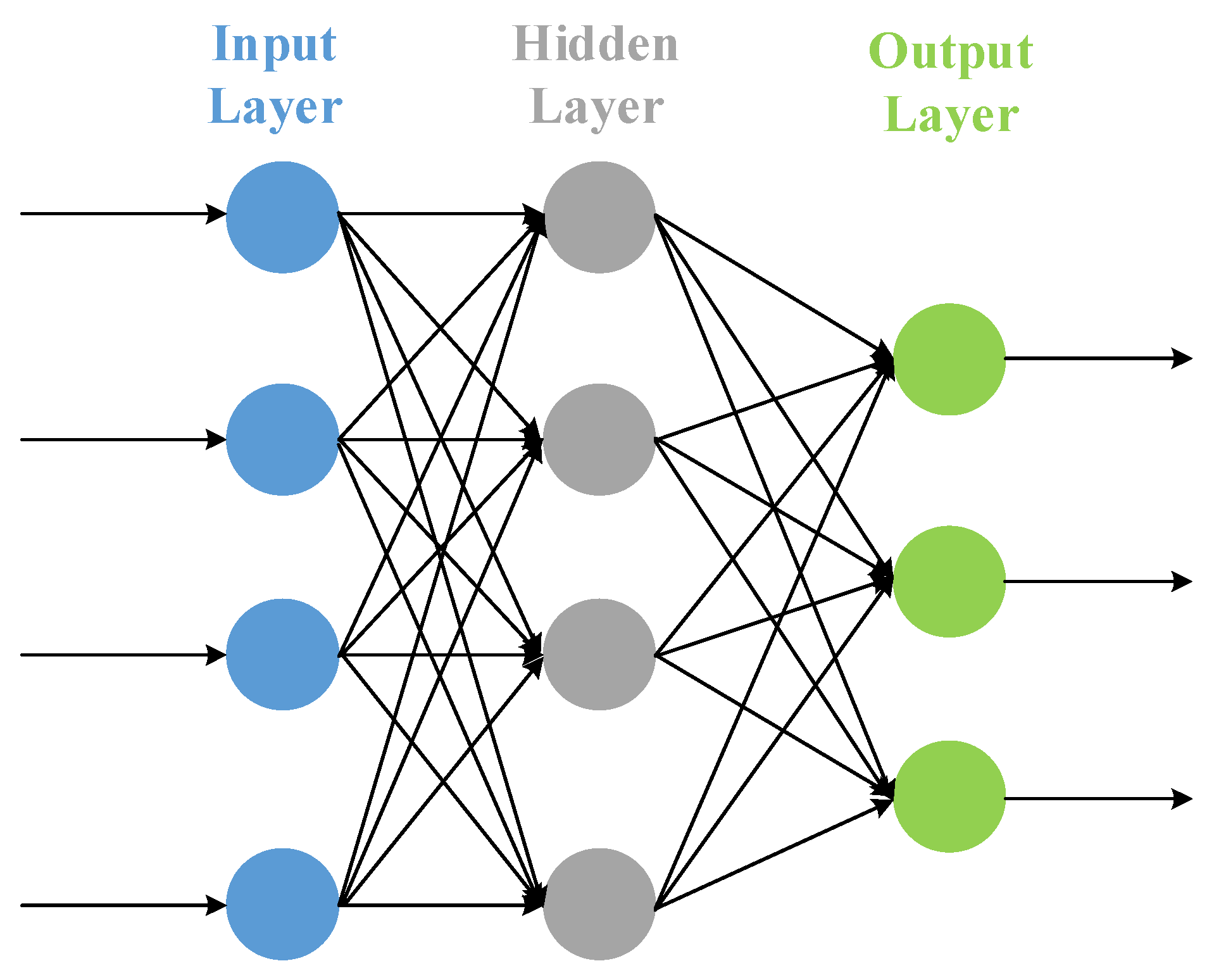
For nonlinear problems, back-propagation neural networks are often utilized to build the models [28,29,30]. In this paper, a typical back-propagation neural network is employed to conduct the evaluation. The typical back-propagation neural network consists of a three-layer framework, i.e., input–hidden–output layer, as is shown in Figure 1.
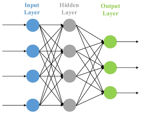
Figure 1.
The structure of the typical back-propagation neural network.
The structure of a neuron is shown in Figure 2. For each neuron, the relationship between the input and the output y can be calculated as:
where is the weight for each input, is to sum up all the inputs and f is the activation function.
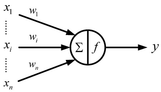
Figure 2.
The structure of an artificial neuron.
2.2. Error Measures
Indicators used for evaluating the performances of APT prediction methods usually include mean error, mean square error (MSE), mean absolute error, mean percentage error and mean percentage absolute error [20,31,32]. For indicators such as mean percentage error and mean absolute percentage error (MAPE), when the value of the indicator reaches a threshold, the predicted results are believed as effective results. For the indicators such as MSE and mean absolute error, the smaller the absolute values of the indicators are, the better the predicted results are believed [33]. Particularly, for APT prediction, the predicted result of the APT in the target year draws great attention, which directly determines the next expansion time of the airport. In this paper, the MAPE is employed as the indicator to verify the adaption of different models for the target year prediction. The MAPE can be obtained by:
where eit is the APT predicting error of the ith airport in tth year, Yit is the APT predicting the result of the ith airport in tth year and yit is the APT observation of the ith airport in tth year.
The acceptable error of the predicted result can be defined as:
where ε is the maximum MAPE that can be accepted. Usually, when eit ≤ 10%, the models are regarded as good models. When eit > 20%, the models are believed to be failure models.
The Civil Aviation Administration of China (CAAC) divides airports into three levels according to the APT of each airport. The distribution of 203 studied airports is shown in Table 1. Since the APT fluctuations of small airports and new airports are usually larger than that of the large airports and the airports under stable operation, ε is set to be 10%, 15% and 20% to study the available models for different types of airports. Four evaluation criteria are set in this paper to see the change of the number of predictable airports after changing the maximum allowable prediction error percentage.

Table 1.
The distribution of 203 studied airports.
3. Data and Hypothesis
For a comprehensive assessment of models for airports under different development conditions, 203 airports in China are studied, which covers various influence factors such as conditions of economic development, conditions of industrial structure and conditions of infrastructure. All the 203 airports have been under operation for at least 5 years, which avoids the impact of APT fluctuation during earlier times. Due to the breaking out of COVID-19, the APT of each airport decreased sharply in 2020 and 2021 [34]. The APT of all the airports in China in 2020 was only 63.3% in comparison to that in 2019, and such conditions will inevitably lead to the failures of all the models. Since the completion times of each airport are diverse from each other, the observations of APT before 2014 are used to fit the initial models. For each airport, the number of observation data for fitting is at least 15, which ensures fitting accuracy. The remaining observations, 2015–2019, are used to evaluate the forecasting performance of the models.
The data for the research can be divided into two types. One is the historical APT observations, which can be obtained from the Civil Aviation Administration of China (CAAC, http://www.caac.gov.cn/en/SY/ (accessed on 22 August 2022)). The other one is the indicators of economic development, which contains gross domestic product (GDP), GDP of primary industry, GDP of secondary industry, GDP of tertiary industry, resident population, year-end population, urbanization rate, imports and exports, disposable income, total retail sales of consumer goods, tourist visits and tourism income. The data can be obtained from the National Bureau of Statistics of China (NBSC, http://www.stats.gov.cn/english/ (accessed on 22 August 2022)).
4. Evaluation Results and Discussion
4.1. The Evaluation Results
The evaluation mainly focuses on the adaption of different prediction models. For each model, the applicable scenes are discussed and the applicable conditions are given. By comparing the numbers of good models for each airport, the authors try to give out the reasons for failures. Considering the significance of results for the target year, four evaluation criteria with different levels of goodness are selected to assess the model suitability of different levels of goodness. Criterion 1: when the maximum mean absolute percentage error (MAPE) satisfies ε ≤ 10%, the model is a good model. Criterion 2: when the maximum MAPE satisfies ε ≤ 15%, the model is a good model. Criterion 3: when the maximum MAPE satisfies ε ≤ 20%, the model is a good model. Criterion 4: when the APT of the airport is more than 10 million and the maximum MAPE satisfies ε ≤ 10%, the model is a good model. When the APT of the airport is between 2 million and 10 million and the maximum MAPE satisfies ε ≤ 15%, the model is a good model. When the APT of the airport is less than 2 million and the maximum MAPE satisfies ε ≤ 20%, the model is a good model. The four criteria are based on different values of MAPE to set different levels of goodness which can be used to show the model suitability of different levels of goodness and to see the change in the number of predictable airports after changing the maximum allowable prediction error percentage.
4.1.1. Time Series Models
For the trend extrapolation models including linear trend, quadratic trend, cubic trend, power trend, exponential trend and logarithmic trend models, the most effective model is firstly determined for a certain airport. The coefficient of determination is used to judge the effectiveness of the models and the model with the largest coefficient of determination is selected as the model for prediction. If the coefficients of determination of all the six models are smaller than 0.8, the trend extrapolation models are deemed to be failed for prediction.
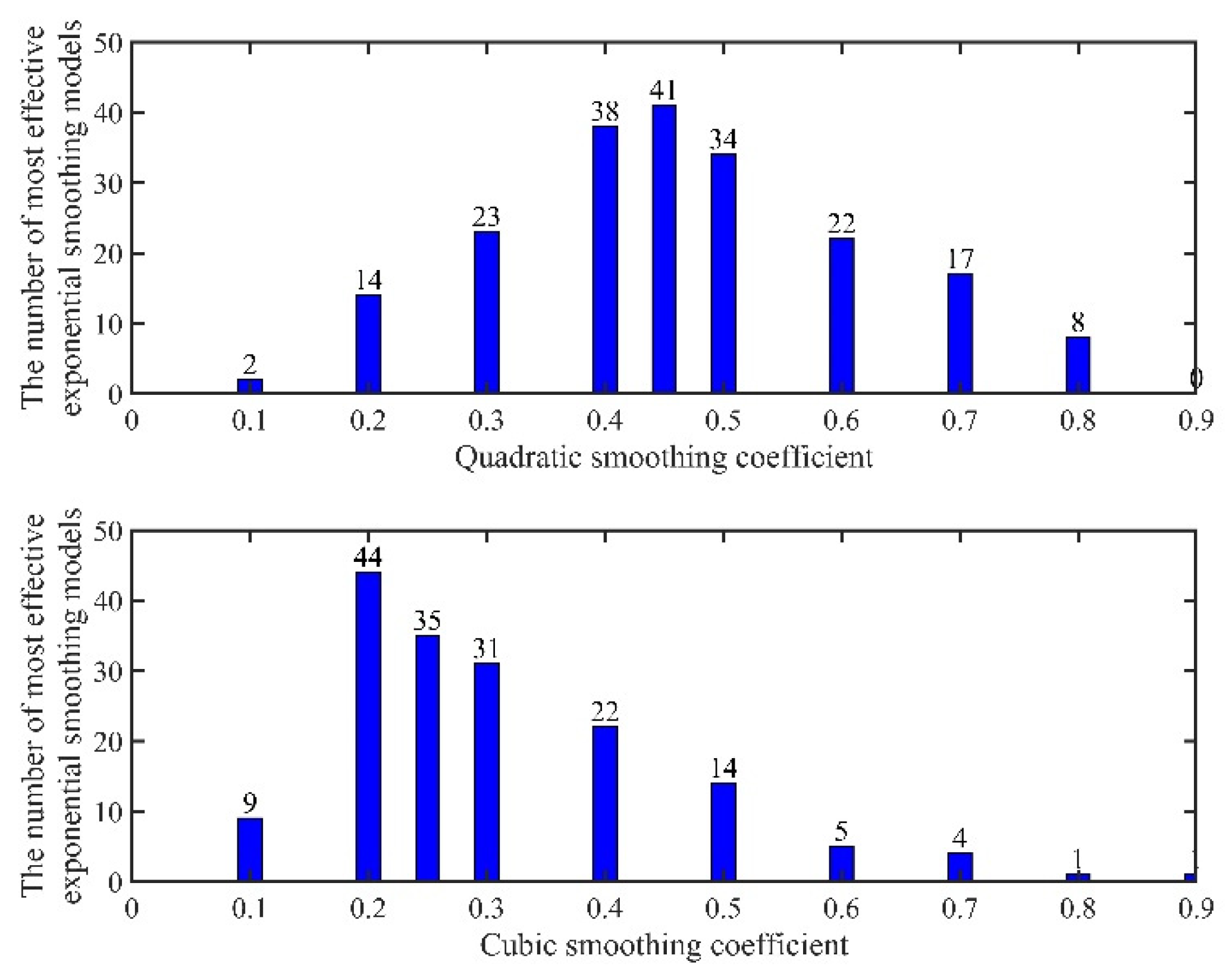
For the exponential smoothing models including quadratic exponential smoothing models and cubic exponential smoothing models, different values of the smoothing coefficients exert a tremendous influence on the predicted results. The most effective exponential smoothing model is determined by computing the MAPE of models under different smoothing coefficients. By setting the MAPE as 10%, the distribution of the number of most effective exponential smoothing models for airports under different smoothing coefficients is shown in Figure 3. For quadratic exponential smoothing models, when the smoothing coefficient is set as 0.45, the corresponding model is suitable for most airports under the given error. When the smoothing coefficient is set as 0.2, the corresponding cubic exponential smoothing model is suitable for most airports under the given error.
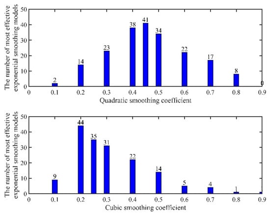
Figure 3.
The distribution of the number of most effective exponential smoothing models.
For the grey models, at least four points are needed to initiate the model which means that the minimum order number of a GM (1,1) is 4. By accumulating the observation sequences, the models are established and the effectiveness of the models is judged by the relative error test, correlation test and posterior difference test.
The evaluating results of the above models are shown in Table 2, from which we can see that the exponential smoothing models perform better than the other two types of models. The exponential smoothing models can be used as good models for 68% of all the 203 airports under all four evaluating criteria. The trend extrapolation models show better performances in larger airports. The grey models can predict accurately for fewer airports because only a few airports show the characteristics of exponential growth.
Table 2.
The evaluating results of the time series models.
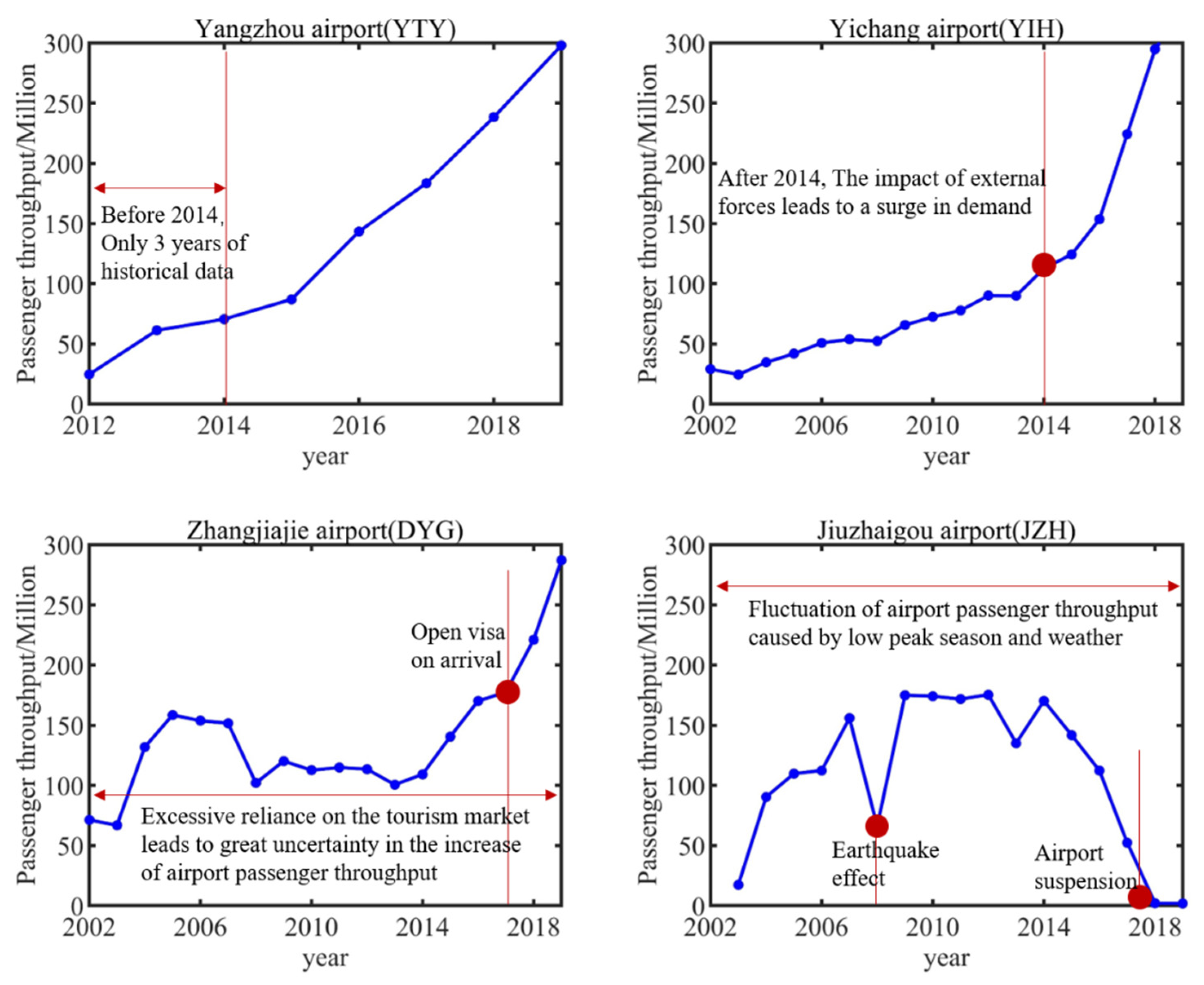
The applicability of the models on different levels of airports is shown in Table 3. The time series models are defined to be effective for an airport when at least one of the models is a good model under the given criterion. For the airports with APT of more than 10 million, 100% of the airports can be predicted effectively. Meanwhile, the time series models show poor applicability to airports with APT of less than 2 million. The criteria do not perform much influence on the predicted results. Considering the unavailability of the time series models, the airports with APT between 2 million and 10 million are studied in detail. There are only three airports that cannot be predicted by the time series models, which are shown in Figure 4. The Yangzhou airport (YTY) started running in 2012 and the little data make the models difficult to fit the observations well. The Yichang airport (YIH) is influenced by the Three Gorges Dam Project and its APT has shown explosive growth since 2014 when the Three Gorges Dam Project was opened to the public. The Zhangjiajie airport (DYG) develops depending much on the tourist industry. At first, the Zhangjiajie airport experienced a rapid expansion owing to the development of tourism resources. Then for a while, the Zhangjiajie airport was affected by the development of the high-speed railway. In 2017, after the visa on arrival was permitted, the APT of the airport returned to positive growth. For the airports with APT less than 2 million, 49 airports cannot be predicted by the time series models. Eighteen airports lack sufficient data. Eight airports suffer from data interruption because of expansion or relocation. The others are driven by external forces and show a lot of uncertainties like the Jiuzhaigou (JZH) airport.
Table 3.
The applicability of time series models on different levels of airports.
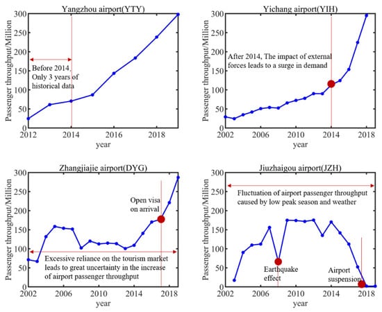
Figure 4.
The four airports which are unavailable predicted by the time series models.
4.1.2. Causal Models
The accuracy of the causal models is mainly influenced by the choices of variables. The relationship between the variables and APT should be first studied. Many studies tried to solve the relationship. Wu et al. [35] analyzed the relationship between APT and indicators of socio-economic development in each province of China. The result showed that the APT was strongly positively correlated with the GDP, urbanization rate and population density and the APT per unit GDP was weakly correlated with the GDP, urbanization rate and population density. In this paper, the relationship is comprehensively researched. GDP, GDP of primary industry, GDP of secondary industry, GDP of tertiary industry, resident population, year-end population, urbanization rate, imports and exports, disposable income, total retail sales of consumer goods, tourist visits and tourism income are selected as the variables. The correlation analysis is conducted on the APT of the airport and the indicators of the province where the airport is located. Usually, when the correlation coefficient between two variables is larger than 0.8, the two variables are believed to be highly correlated. The correlation coefficients between APT and each indicator are shown in Table 4. It is shown that the APT of an airport is highly correlated to the GDP of the city where the airport is located. In addition, the higher the magnitude of airport passenger throughput, the better the correlation between passenger throughput and macro indicators.
Table 4.
The correlation coefficients between APT and indicators.
To exclude the influence of correlation between the indicators, the correlation between GDP and the other indicators is also studied and the results are shown in Table 5. It is shown that GDP is strongly correlated with the GDP of secondary industry, GDP of tertiary industry, disposable income and total retail sales of consumer goods.
Table 5.
The correlation coefficients between GDP and the other indicators.
For the regression models, the effectiveness of the models is determined by the coefficient of determination. The more the coefficient of determination is close to 1, the better the model is. Usually, the model is regarded as an effective model when the coefficient of determination is larger than 0.8. In this paper, the F inspection value and t inspection value at the significance level of 0.95 are also employed.
For unary linear regression models, the results of all 12 indicators are calculated. As shown in Table 6, the predicting results of unary linear regression models do not perform well although by using the coefficient of determination the variables are highly correlated to the APT of most airports. It can be found that GDP, GDP of tertiary industry, disposable income, total retail sales of consumer goods, tourist visits and tourism income highly affect the effectiveness of all the models.
Table 6.
The evaluating results of unary linear regression models.
For stepwise regression models, by using all 12 indicators as the input variables, the predicting performance may be influenced by the correlation between the indicators although the significance level of the model is guaranteed by the model’s building process. Therefore, GDP, GDP of tertiary industry, disposable income, total retail sales of consumer goods, tourist visits and tourism income are selected as the limited inputs to build the models as well. As is shown in Table 7, the strategy of using limited inputs performs better.
Table 7.
The evaluating results of stepwise regression models.
For the hybrid regression causal models, each model is built using the most correlated variable and the evaluating results are shown in Table 8.
Table 8.
The evaluating results of the hybrid regression causal model.
For the elastic coefficient models, GDP, GDP of tertiary industry, disposable income, total retail sales of consumer goods, tourist visits and tourism income are selected as the correlated factors and the evaluating results are shown in Table 9. The results indicate that the models using GDP, GDP of tertiary industry, disposable income and total retail sales of consumer goods perform better.
Table 9.
The evaluating results of elastic coefficient models.
For the proposed elastic-like scale models, the GDP, tourist visits, and resident population are chosen as the indicators. The effectiveness of the regression models is defined as any one of the unary linear regression models, stepwise regression models and hybrid regression models that can predict the APT of an airport effectively. The effectiveness of the elastic coefficient models is defined as any one of the elastic coefficient models that can predict the APT of an airport effectively. Then, the performances of regression models, elastic coefficient models and the elastic-like scale models can be compared, as shown in Table 10.
Table 10.
The comparison of the causal models.
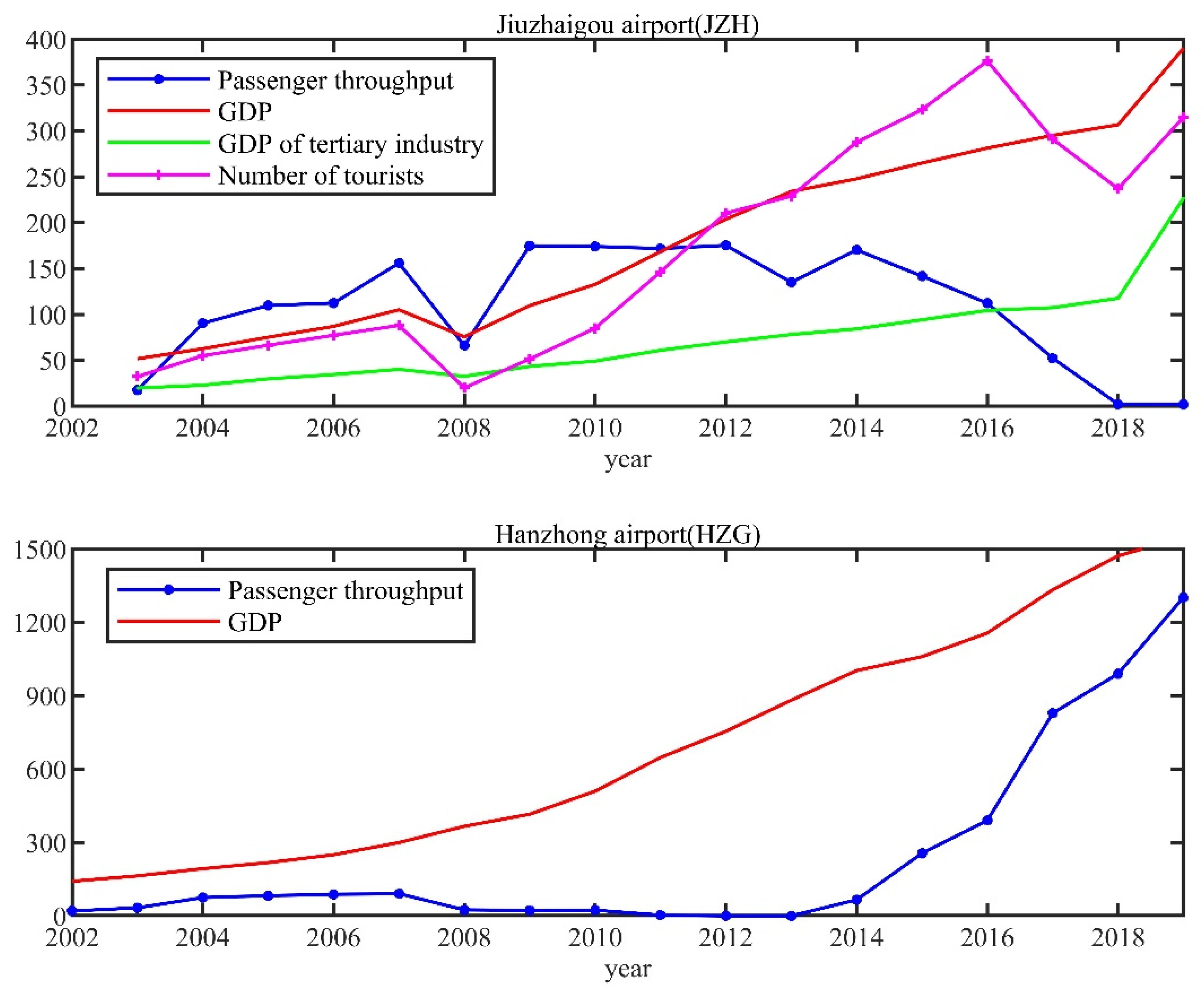
As shown in Table 11, the applicability of the causal models on different airport levels shows that 80% of airports can use the causal models to predict. For airports with APT of more than 2 million, the models can be used to predict 100% of airports. For those that cannot be predicted, the APT of the airports shows characteristics including inconsistent trending of APT and economic development, lower correlation between the APT and economic indicators and incoherent observations because of stopping the service, as shown in Figure 5.
Table 11.
The applicability of causal models on different levels of airports.
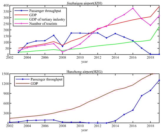
Figure 5.
The airports cannot be predicted by the causal models.
4.1.3. Market Share Methods
For all 203 airports, each airport is located in a city without other airports except in the cities of Beijing, Shanghai and Chengdu, which means that for most of the airports, the market shares of the airports are the same as the market shares of the cities when using the market share method. The market share methods can be used to calculate the APT of airports accounting for the province’s market share, the APT of airports accounting for the nation’s market share, as well as the APT of airports accounting for the city agglomeration’s market share. Since the 19 city agglomerations in China only cover 121 airports, the corresponding method is suitable for 121 airports. The market shares are fitted by using the time series models and the evaluating results are shown in Table 12.
Table 12.
The evaluating results of market share methods.
By evaluating the criteria proposed, the applicability of the market share methods on different airport levels is listed in Table 13. Generally, the market share methods are effective in 70% of airports. Under different criteria, the effectiveness does not fluctuate a lot. By checking the applicability of the market share methods on different levels of airports, the market share methods can predict the airports with APT of more than 10 million accurately except for the Ningbo airport under Criterion 1. For airports with APT between 2 million and 10 million, the airports can all be predicted except for the Yangzhou airport, Yichang airport and Zhangjiajie airport under Criterion 1. Overall, 60% of the airports with APT less than 2 million can be predicted effectively. For the airports which are cannot be predicted by the market share methods, the observations of 18 airports are too less to fit the models, and the others fluctuate disorderly because their own development regularity is not strong enough like Baotou airport (BAV) shown in Figure 6. The unpredictable airports are all located in remote areas. Comparing the performances of time series models with market share methods, the predictive abilities of the two kinds of methods are nearly the same, which is shown in Table 14. The airports which can be predicted by the time series models but cannot be predicted by the market share methods are shown in Table 15.
Table 13.
The applicability of the market share method on different levels of airports.
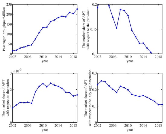
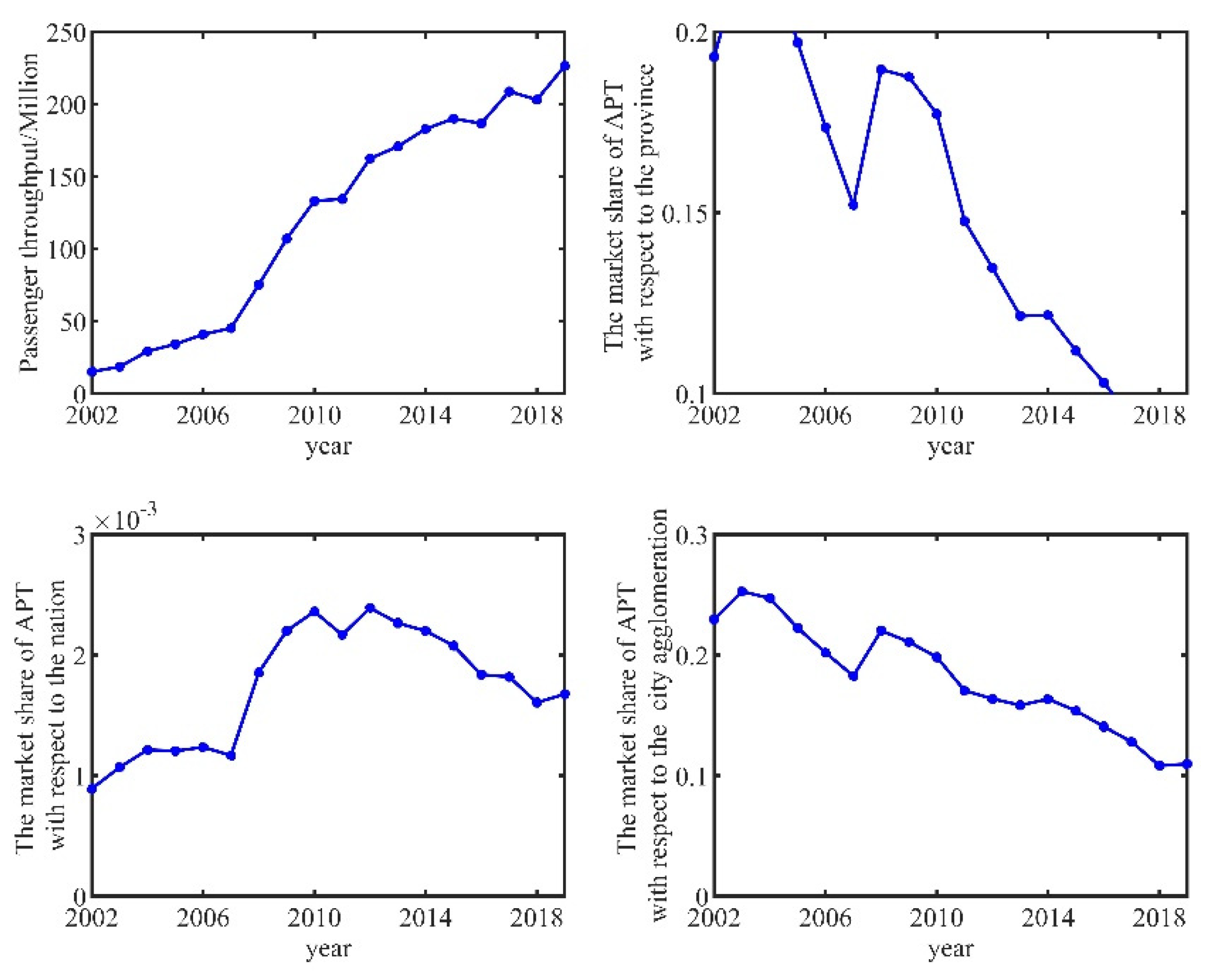
Figure 6.
Market share of Baotou airport (BAV).
Table 14.
Comparison of the time series models and the market share methods.
Table 15.
The airports that can be predicted by the time series models but cannot be predicted by the market share methods.
4.1.4. Analogy-Based Method
According to the constructing process of the analogy-based method proposed in Section 2, the APT of all 203 airports can be used as the database for analogy. The target airports for analogy are determined by the levels of the focusing airports. The evaluation results of the analogy-based method on different levels of airports are shown in Table 16.
Table 16.
The applicability of analogy-based method on different levels of airports.
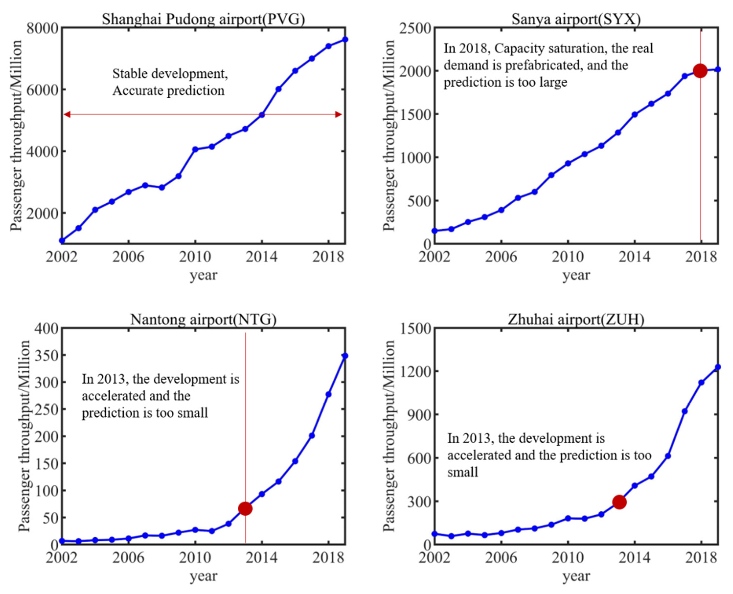
Generally, compared with time series models, causal models and market share methods, the performance of the analogy-based method is worse, especially for the smaller airports. In addition, under different criteria, the performances are quite different, which indicates that the prediction accuracy of the analogy-based method is relatively low. By analyzing the applicable scenes of the analogy-based method, it is found that the analogy-based method is more suitable for the APT with a linear trend like Shanghai Pudong Airport (PVG) shown in Figure 7. When the increasing rate of APT is small, the predicted result will be relatively larger than the observation like Sanya Airport (SYX). When the increasing rate of APT is small, the predicted results will be relatively smaller than the observation of Nantong Airport (NTG) and Zhuhai Airport (ZUH).
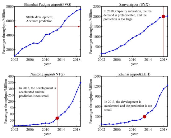
Figure 7.
The applicable scenes of the analogy-based methods.
4.1.5. Artificial Intelligent Models
The artificial intelligent models are built using the neural network toolbox provided by MATLAB. A feedforward neural network with 12 inputs, 1 output and 10 neurons in the hidden layer is first built. The best performance appears when the training function is set to be ‘trainlm’. Compared with the other proposed models, the artificial intelligent model performs worst. Only 10% of all the airports can be predicted by the neural network. The evaluating results of the artificial intelligent model on different airport levels are shown in Table 17.
Table 17.
The applicability of the artificial intelligent model on different levels of airports.
4.2. Analysis and Discussion of the Hybrid Method
The APT of an airport is deemed to be effectively predicted when there is at least one of five proposed models can be used to predict the APT effectively for each airport under arbitrary criteria and the hybrid five-model method is applicable. Approximately 180 of 203 tested airports can be effectively predicted and the total predictable proportion is about 88% under Criterion 1. It reveals that the hybrid method combining the time series model, the causal model, the artificial intelligent model, the market share model and the analogy-based model is applicable to most airports. The unpredictable airports of the five-model hybrid method can generally be divided into two categories. One is because there are insufficient historical data for modelling. The other one is because the APT of the airports changes abruptly owing to expansion, relocation or other kinds of external forces such as earthquakes.
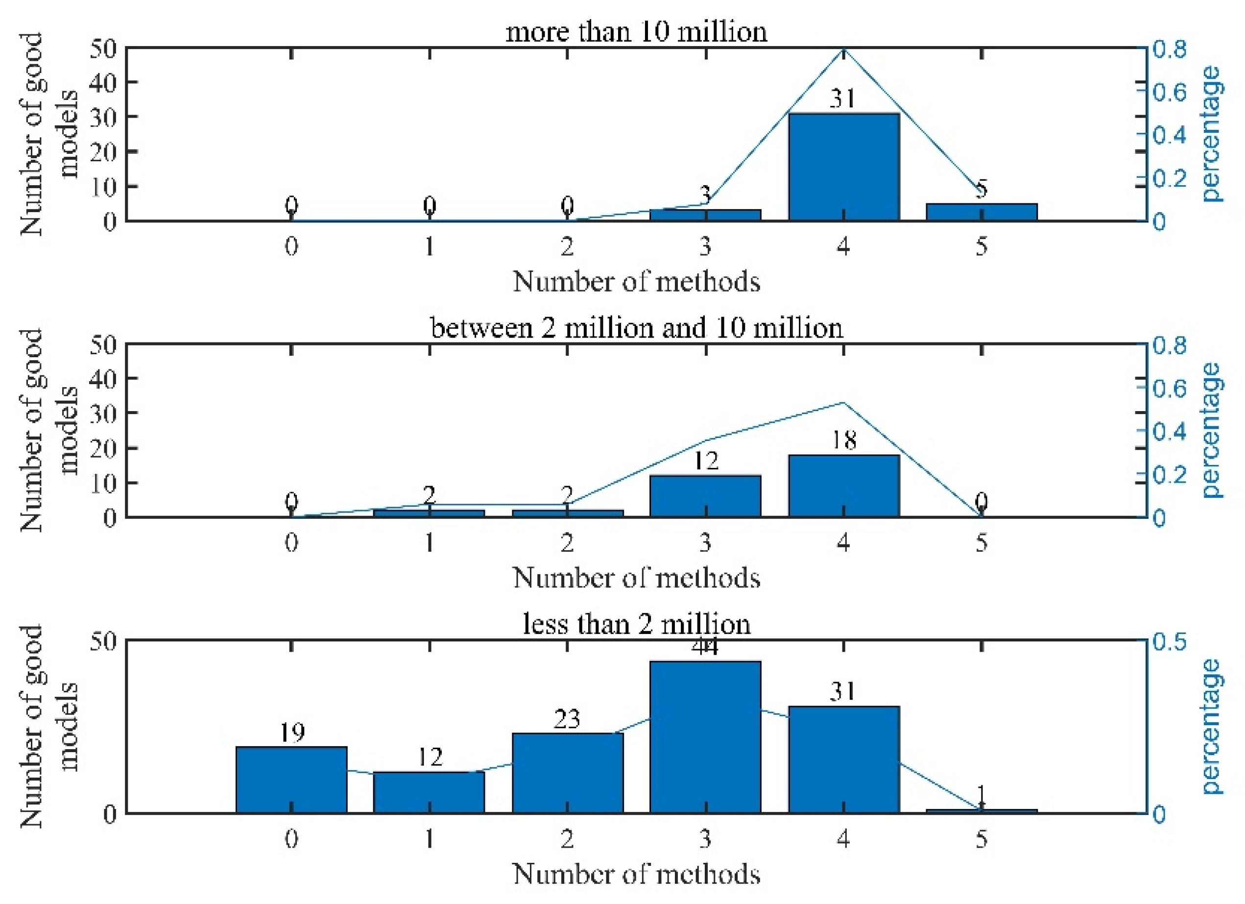
For different levels of airport, all airports with APT of more than 10 million can be effectively predicted under arbitrary criteria with the five-model hybrid method. Regardless of the Zhangjiajie airport (DYG), all the airports with APT between 2 million and 10 million can be effectively predicted under Criterion 1. Under Criterion 2, all the airports with APT between 2 million and 10 million can be effectively predicted. For the airports with APT less than 2 million, 85% of the airports can be effectively predicted. By comparing the number of good models for each airport shown in Figure 8, there are usually more than three good models for the airports with APT of more than 10 million under Criterion 3. For the airports with APT between 2 million and 10 million, there is at least one good model. The applicability of all the models is promoted with the increasing APT. The applicability of all the models on different levels of airports is shown in Table 18. It reveals that large airports with high APT usually have high prediction accuracy with the hybrid evaluating method. Airports with low APT are hard to be predicted with the promoted hybrid evaluating method.

Figure 8.
The distribution of the good models.
Table 18.
The applicability of all the models on different levels of airports.
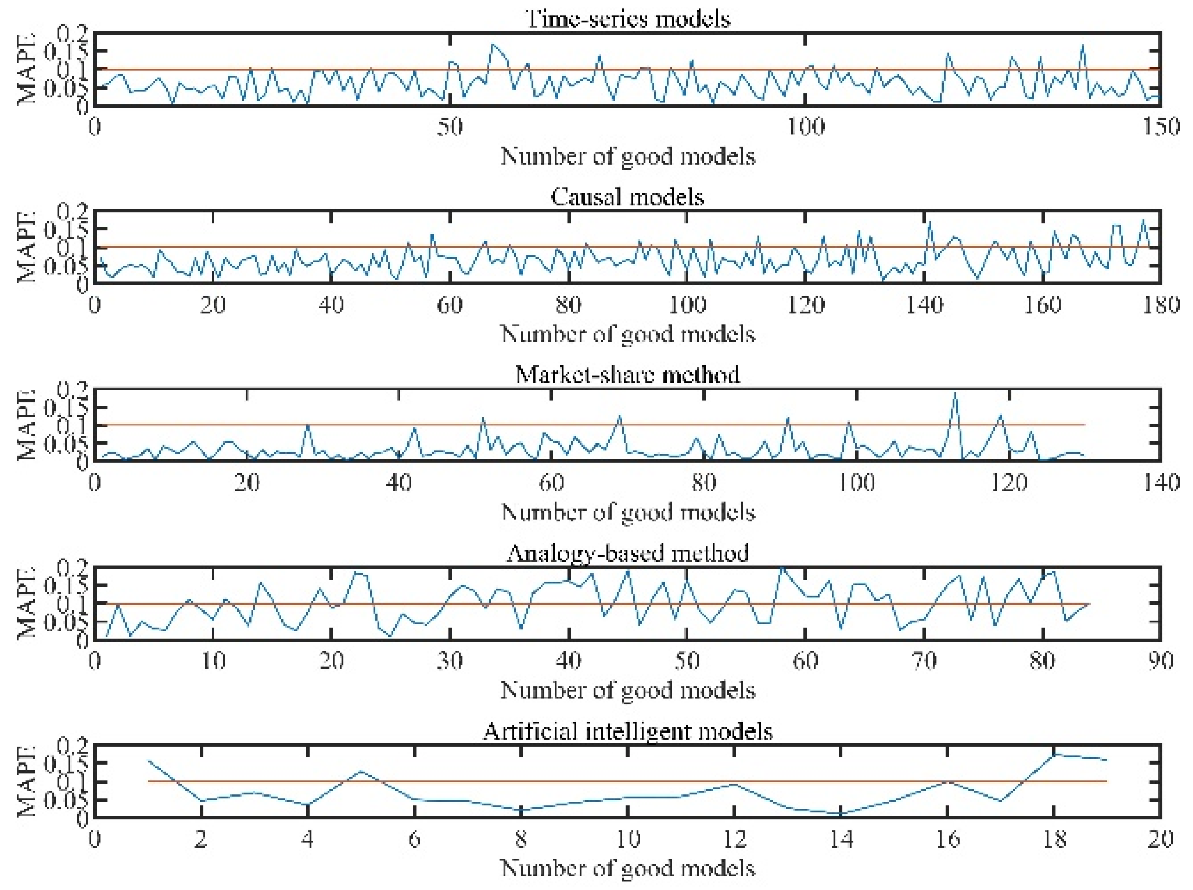
Considering the errors of the effective models, the MAPE performances of the models are given in Figure 9 and Table 19. For airports with APT of more than 10 million, the MAPE is usually smaller than that for the small airports. The MAPEs of time series models, causal models and market share method are less than 10%.
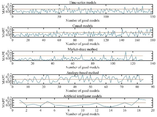
Figure 9.
The MAPE distribution of the effective models.
Table 19.
The prediction performances of the effective models according to MAPE.
5. Conclusions
Time series models, causal models, artificial intelligent models, market share methods and analogy-based methods are all commonly used methods for APT prediction. In the paper, a hybrid method of the aforementioned methods is developed and investigated. By conducting the evaluation of five kinds of models to predict the APT of two hundred three airports in China, it is found that for most prediction scenes, the models are applicative to the short-term prediction of APT and the accuracy does not improve with the complexities of the models. Overall, 88% of the studied airports can be effectively predicted by using the evaluated prediction methods, and the MAPE is mostly within 10%. In addition, the constructed evaluation method can effectively predict the airport passenger throughput of more than 10 million. The higher the airport passenger throughput level is, the more effective the segmentation prediction methods can be. The performance of the mentioned models in this paper is bad when there are insufficient historical data for modelling, or the APT of the airports changes abruptly owing to expansion, relocation or other kinds of external forces like earthquakes. When the airport enters the stable development period, the number of available prediction models in the hybrid method is significantly increased. The results show that there is no relationship between the prediction accuracy and the complexity of prediction models. Among the five used models, the time series model, causal models and market share method usually have higher applicability than the other two models. The findings provide potential support for the selection of prediction models for the APT prediction. The prediction and evaluation methods in this paper are usually applicable to airports with high APT, stable development periods and sufficient historical data. Further studies should be made to build prediction and evaluation methods when the external environment is unstable under the influence of COVID-19 and other external forces such as earthquakes or without sufficient historical data.
Author Contributions
Conceptualization, B.C. and J.W.; methodology, B.C.; software, B.C.; validation, B.C., J.W. and X.Z.; formal analysis, X.Z.; investigation, B.C.; resources, B.C.; data curation, B.C.; writing—original draft preparation, B.C.; writing—review and editing, X.Z.; visualization, X.Z.; supervision, J.W. and X.Z.; project administration, J.W. and X.Z.; funding acquisition, J.W. and X.Z. All authors have read and agreed to the published version of the manuscript.
Funding
This research was funded by the project “Civil Aviation Safety Capacity Enhancement Project”, which is supported by the Civil Aviation Administration of China.
Institutional Review Board Statement
Not applicable.
Informed Consent Statement
Not applicable.
Data Availability Statement
Not applicable.
Acknowledgments
The authors gratefully acknowledge the financial support provided by the project “Civil Aviation Safety Capacity Enhancement Project”, which is supported by the Civil Aviation Administration of China.
Conflicts of Interest
The authors declare no conflict of interest.
References
- Solvoll, G.; Mathisen, T.A.; Welde, M. Forecasting air traffic demand for major infrastructure changes. Res. Transp. Econ. 2020, 82, 100873. [Google Scholar] [CrossRef]
- Kurdel, P.; Sedláčková, A.N.; Novák, A. Analysis of Using Time Series Method for Prediction of Number of Passengers at the Airport. J. KONBiN 2020, 50, 203–216. [Google Scholar] [CrossRef]
- Cheng, L.; Xiao, M. A Review of Research on Airline Passenger Volume Forecasting. In Proceedings of the 2017 4th International Conference on Machinery, Materials and Computer (MACMC 2017), Xi’an, China, 27–29 November 2017. [Google Scholar]
- Zhang, X. Research on forecasting method of aviation traffic based on social and economic indicators. IOP Conf. Ser. Mater. Sci. Eng. 2020, 780, 062038. [Google Scholar] [CrossRef]
- Peng, D.; Zhang, M.; Xiao, Y.; Wang, Y. Research on Passenger Throughput Forecast of Civil Aviation Airport Based on Multi-source Data. J. Phys. Conf. Ser. 2022, 2179, 012027. [Google Scholar] [CrossRef]
- Bastola, D.P. Air Passenger Demand Model (APDM): Econometric Model For Forecasting Demand In Passenger Air Transports In Nepal. Int. J. Acad. Res. Psychol. 2017, 1, 238–242. [Google Scholar]
- Jin, F.; Li, Y.; Sun, S.; Li, H. Forecasting air passenger demand with a new hybrid ensemble approach. J. Air Transp. Manag. 2019, 83, 101744. [Google Scholar] [CrossRef]
- Xie, G.; Wang, S.; Lai, K.K. Short-term forecasting of air passenger by using hybrid seasonal decomposition and least squares support vector regression approaches. J. Air Transp. Manag. 2014, 37, 20–26. [Google Scholar] [CrossRef]
- Xu, S.; Chan, H.K.; Zhang, T. Forecasting the demand of the aviation industry using hybrid time series SARIMA-SVR approach. Transp. Res. Part E Logist. Transp. Rev. 2018, 122, 169–180. [Google Scholar] [CrossRef]
- Gunter, U.; Zekan, B. Forecasting air passenger numbers with a GVAR model. Ann. Tour. Res. 2021, 89, 103252. [Google Scholar] [CrossRef]
- Scarpel, R.A. Forecasting air passengers at São Paulo International Airport using a mixture of local experts model. J. Air Transp. Manag. 2013, 26, 35–39. [Google Scholar] [CrossRef]
- Zhou, W.; Cheng, Y.; Ding, S.; Chen, L.; Li, R. A grey seasonal least square support vector regression model for time series forecasting. ISA Trans. 2020, 114, 82–98. [Google Scholar] [CrossRef]
- Wong, H.L. Time Series Forecasting with Stochastic Markov Models Based on Fuzzy Set and Grey Theory. Appl. Mech. Mater. 2015, 764–765, 975–978. [Google Scholar] [CrossRef]
- Liang, X.; Zhang, Q.; Hong, C.; Niu, W.; Yang, M. Do Internet Search Data Help Forecast Air Passenger Demand? Evidence From China’s Airports. Front. Psychol. 2022, 13, 809954. [Google Scholar] [CrossRef]
- Li, X.; Groot, M.D.; Bck, T. Using forecasting to evaluate the impact of COVID-19 on passenger air transport demand. Decis. Sci. 2021. [Google Scholar] [CrossRef]
- Barczak, A.; Dembińska, I.; Rozmus, D.; Szopik-Depczyńska, K. The Impact of COVID-19 Pandemic on Air Transport Passenger Markets-Implications for Selected EU Airports Based on Time Series Models Analysis. Sustainability 2022, 14, 4345. [Google Scholar] [CrossRef]
- Karlaftis, M.G.; Zografos, K.G.; Papastavrou, J.D.; Charnes, J.M. Methodological Framework for Air-Travel Demand Forecasting. J. Transp. Eng. 1996, 122, 96–104. [Google Scholar] [CrossRef]
- Maldonado, J. Strategic Planning—An Approach to Improving Airport Planning under Uncertainty. Master’s Thesis, Massachusetts Institute of Technology, Cambridge, MA, USA, 1990. [Google Scholar]
- Mierzejewski, E.A. A New Strategic Urban Transportation Planning Process; Center for Urban Transportation Research, University of South Florida: Tampa, FL, USA, 1995. [Google Scholar]
- Odeck, J.; Welde, M. The accuracy of toll road traffic forecasts: An econometric evaluation. Transp. Res. Part A Policy Pract. 2017, 101, 73–85. [Google Scholar] [CrossRef]
- Flyvbjerg, B.; Holm, M.K.S.; Buhl, S.L. How (In)accurate Are Demand Forecasts in Public Works Projects?: The Case of Transportation. J. Am. Plan. Assoc. 2005, 71, 131–146. [Google Scholar] [CrossRef]
- Nicolaisen, M.S.; Driscoll, P.A. Ex-Post Evaluations of Demand Forecast Accuracy: A Literature Review. Transp. Rev. 2014, 34, 540–557. [Google Scholar] [CrossRef]
- Djakaria, I. Djalaluddin Gorontalo Airport Passenger Data Forecasting with Holt’s-Winters’ Exponential Smoothing Multiplicative Event-Based Method. J. Phys. Conf. Ser. 2019, 1320, 012051. [Google Scholar] [CrossRef]
- Kochkina, E.; Radkovskaya, E.; Denezhkina, K. Analysis and forecasting of performance indicators of air transport facilities. E3S Web Conf. 2021, 291, 08009. [Google Scholar] [CrossRef]
- Priyadarshana, M. Modeling Air Passenger Demand in Bandaranaike International Airport, Sri Lanka. J. Bus. Econ. Policy 2015, 2, 146–151. [Google Scholar]
- Zhang, F.; Graham, D.J. Air transport and economic growth: A review of the impact mechanism and causal relationships. Transp. Rev. 2020, 40, 506–528. [Google Scholar] [CrossRef]
- Goldfarb, R.S.; Stekler, H.O.; David, J. Methodological issues in forecasting: Insights from the egregious business forecast errors of late 1930. J. Econ. Methodol. 2005, 12, 517–542. [Google Scholar] [CrossRef]
- Wang, J.Z.; Wang, J.J.; Zhang, Z.G.; Guo, S.P. Forecasting stock indices with back propagation neural network. Expert Syst. Appl. 2011, 38, 14346–14355. [Google Scholar] [CrossRef]
- Jiang, X.; Zhang, Y.; Li, Y.; Zhang, B. Forecast and analysis of aircraft passenger satisfaction based on RF-RFE-LR model. Sci. Rep. 2022, 12, 11174. [Google Scholar] [CrossRef]
- Cheng, L.; Liu, L.; Xiao, B. Artificial Neural Networks Method for Predicting the Airport Passenger Throughput. Aeronaut. Comput. Tech. 2000, 30, 8–11. [Google Scholar]
- Wang, Z.; Song, W.K. Sustainable airport development with performance evaluation forecasts: A case study of 12 Asian airports. J. Air Transp. Manag. 2020, 89, 101925. [Google Scholar] [CrossRef]
- Profillidis, V. An ex-post assessment of a passenger demand forecast of an airport. J. Air Transp. Manag. 2012, 25, 47–49. [Google Scholar] [CrossRef]
- Liu, S.Y.; Liu, S.; Tian, Y.; Sun, Q.L.; Tang, Y.Y. Research on Forecast of Rail Traffic Flow Based on ARIMA Model. J. Phys. Conf. Ser. 2021, 1792, 012065. [Google Scholar] [CrossRef]
- Kitsou, S.P.; Koutsoukis, N.S.; Chountalas, P.; Rachaniotis, N.P. International Passenger Traffic at the Hellenic Airports: Impact of the COVID-19 Pandemic and Mid-Term Forecasting. Aerospace 2022, 9, 143. [Google Scholar] [CrossRef]
- Xiangli, W.U.; Man, S. Air transportation in China: Temporal and spatial evolution and development forecasts. J. Geogr. Sci. 2018, 28, 1485–1499. [Google Scholar]

Disclaimer/Publisher’s Note: The statements, opinions and data contained in all publications are solely those of the individual author(s) and contributor(s) and not of MDPI and/or the editor(s). MDPI and/or the editor(s) disclaim responsibility for any injury to people or property resulting from any ideas, methods, instructions or products referred to in the content. |
© 2023 by the authors. Licensee MDPI, Basel, Switzerland. This article is an open access article distributed under the terms and conditions of the Creative Commons Attribution (CC BY) license (https://creativecommons.org/licenses/by/4.0/).