Low-Cost Handheld Spectrometry for Detecting Flavescence Dorée in Vineyards

Abstract

This study was conducted to evaluate the potential of low-cost hyperspectral sensors for the early detection of Flavescence dorée (FD) from asymptomatic samples prior to symptom development. In total, 180 leaf spectra from 60 randomly selected plants (three leaves per plant) were collected by using two portable mini-spectrometers (Hamamatsu: 340–850 nm and NIRScan: 900–1700 nm) at five vegetative growth stages in a vineyard with grape variety Garganega. High differences in the Hamamatsu spectra of the two groups were found in the VIS-NIR (visible–near infrared) spectral region while very small differences were observed in the NIRScan spectra. We analyzed the spectral data of two sensors by using all bands, features reduced by an ensemble method, and by genetic algorithms (GA) to discriminate the asymptomatic healthy (FD negative) and diseased (FD positive) leaves using five different classifiers. Overall, high classification accuracies were found in case of the Hamamatsu sensor compared to the NIRScan sensor. The feature selection techniques performed better compared to all bands, and the highest classification accuracy of 96% was achieved when GA features of the Hamamatsu sensor were used with the logistic regression (LR) classifier on test samples. A slightly low accuracy of 85% was achieved when the features (selected by the ensemble method) of the Hamamatsu sensor were used with the support vector machine (SVM) classifier by using leave-one-out (LOO) cross-validation on the whole dataset. Results demonstrated that employing a feature selection technique can provide a valid tool for determining the optimal bands that can be used to identify FD disease in the vineyard. However, further validation studies are required, as this study was conducted using a small dataset and from the single grapevine variety.

1. Introduction

Flavescence dorée (FD), is a highly epidemic and incurable disease affecting vineyards in various European countries [1]. FD is caused by phytoplasmas, i.e., phloem-limited, non-culturable microorganisms belonging to the 16Sr-V Mollicutes taxonomic group transmitted in the field mainly by the leafhopper Scaphoideus titanus Ball (Hemiptera: Cicadellidae) [2]. In recent years, the disease has been widely spreading especially in north Italian grapevine-growing areas [3], with severe epidemic outbreaks. The disease causes a strong reduction in the quantity and quality of the product and leads to the removal of the affected plants in large areas, with a serious economic impact on the viticulture sector [4,5,6].

FD phytoplasma (FDp) is included in the list of quarantine pathogens in Europe and is therefore subjected to compulsory eradication measures, but the timely identification of infected plants is complicated by several factors. Visual inspection is incapable of detecting the early stages of disease development and is impractical in large fields [4]; similar symptoms caused by other non-quarantine pathogens, namely the Bois Noir phytoplasma (BNp), may be misleading; the timing of symptoms’ appearance may vary among seasons and varieties [7]. As a consequence, infected plants may escape early removal and become inoculum sources for neighboring plants, while non-infected plants with similar symptoms may be unnecessarily removed. A reliable diagnosis can only be achieved following molecular detection of pathogen DNA, by polymerase chain reaction (nested PCR) or quantitative real-time PCR [1]. These lab-based methods involve destructive sampling, are time-consuming and expensive, and require skilled personnel to be carried out in a reliable, sensitive, and versatile manner.

The recent advancements in sensor technologies including hyperspectral spectrometers together with machine learning (ML) methods boost their applications in precision agriculture [8]. ML methods are based on computational algorithms that can learn from the input data and perform classification or clustering tasks, which are suitable to identify the patterns and trends of large amounts of data such as hyperspectral data. In this regard, optical sensing technology has proved to be a potentially very useful tool that used in precision agriculture especially for the diagnosis of plant diseases before they become visible to the human eye [9,10,11,12]. This optical technology and novel sensors measure the reflectance characteristics of plants in different regions of the electromagnetic spectrum by evaluating the interaction between plant leaves and incoming solar radiation. The reflectance (the ratio between the intensities of incoming and reflected light) provides information about the leaf health status and allows to detect the first changes in the physiology of plants caused by biotic stresses. The reflectance of the leaves in the visible spectral regions (VIS) is related to leaf pigment contents and the reflectance in near infrared (NIR) is typically related to leaf cell structure and water contents [13,14,15]. FD infection is known to cause metabolic alterations in grapevine leaves [16] which in turn can alter the foliar optical properties several days before the appearance of the first visible symptoms on the leaves. The high dimensionality of the hyperspectral data is a critical factor that needs to be carefully considered when analyzing the hyperspectral data [17]. High dimensionality of the datasets can be effectively reduced (also called feature selection) by searching for a subset of wavebands containing salient spectral information and by removing non-pertinent, noisy, and redundant features [18]. Al-Saddik et al. [19] exploited GA to investigate the optimal spectral bands to be selected for FD. In another study, Barjaktarović et al. [20] presented in-house developed multispectral camera and highlighted the importance of feature selection approach to select most the optimal spectral bands to detect FD in vineyards.

Several studies have demonstrated the potential of the optical sensor to detect disease FD in grapevines [4,6,21,22]. Al-Saddik et al. [4] investigated the optimal spectral bands for designing a FD-specific spectral sensor to detect the FD in the grapevine field. In this study, authors used feature selection techniques based on the successive projection algorithm (SPA) and the traditional vegetation indices (SVIs) for determining the optimal bands that are sensitive to FD symptomatic plants. Albetis et al. [21] tested the potential of SVIs calculated from a UAV multispectral sensor (MicaSense RedEdge-MX™, MicaSense, Inc., Northlake Way, Seattle, WA, USA) and biophysical parameters (pigment content) to detect abnormal vegetation behaviour in relation to FD and grapevine trunk diseases at various levels of infections. The authors demonstrated that SVIs based on red and green spectral bands effectively map the infected plants when their level of infection is greater than 50%. Likewise in a recent study, Daglio et al. [22] highlighted the potential of using a ground-based multispectral sensor (OptRx^®—Ag Leader, South Riverside Drive Ames, IA, USA) to detect the FD and proposed SVIs which are sensitive to detect the FD. The authors of the study used two SVIs (normalized difference vegetation index: NDVI and normalized difference red-edge index: NDRE) and reported that the infected plants showed lower values compared to healthy plants. However, these studies were conducted either at a single point during the symptomatic phase of the disease or used multispectral sensors with few bands.

The ground-based optical spectroscopy together with ML methods is an interesting approach for rapid monitoring of crop operations and especially plant disease detection [8] but at the same time, there are some constraints to using hyperspectral sensors including portability and their greater equipment cost [23]. Recent advances in field-based spectroscopy have emerged to develop low-cost portable hyperspectral spectrometer devices that provide spectral data for rapid field-based assessments of plant health status. In this regard, many authors presented studies in which they highlighted the necessity to develop such low-cost spectrometer devices which can be used as an alternative to an expensive and time-consuming wet-chemistry analysis.

The aim of this study is to ascertain whether the spectral features extracted from asymptomatic samples could be used to differentiate healthy vines from diseased vines. In the present study, we demonstrate the ability of low-cost hyperspectral sensors combined with ML algorithms for rapid, and cost-effective in-field automated detection of the FD disease. The specific objectives of the study are:

• To compare the performances of the two portable mini spectrometers to detect the FD in vineyards.
• To compare the performance of different machine learning methods for the classification of healthy and infected plants with FD at different stages of disease development.
• To compare the best wavelengths selected by different feature selection methods.

2. Materials and Methods

The study was conducted in the 2022 growing season, in a vineyard located in San Giovanni Ilarione (Verona Province, Italy, 45°31’9” N, 11°14’13” E) at 194 m a.s.l., planted in 2005 with the local grape variety Garganega with a pergola trellising system. The vineyard was selected based on the detection of phytoplasmic symptoms in previous surveys carried out by expert local personnel. For this study, 3 rows for a total of 60 grapevine plants were selected for data acquisition for spectral and PCR analyses (Figure 1C). Plants were visually inspected and scored for symptoms of phytoplasmoses and of other diseases (mainly esca dieback and viral infections) by a plant pathologist from the University of Verona, Italy, on 4 different dates (30 May, 22 June, 28 June, and 7 September 2022).

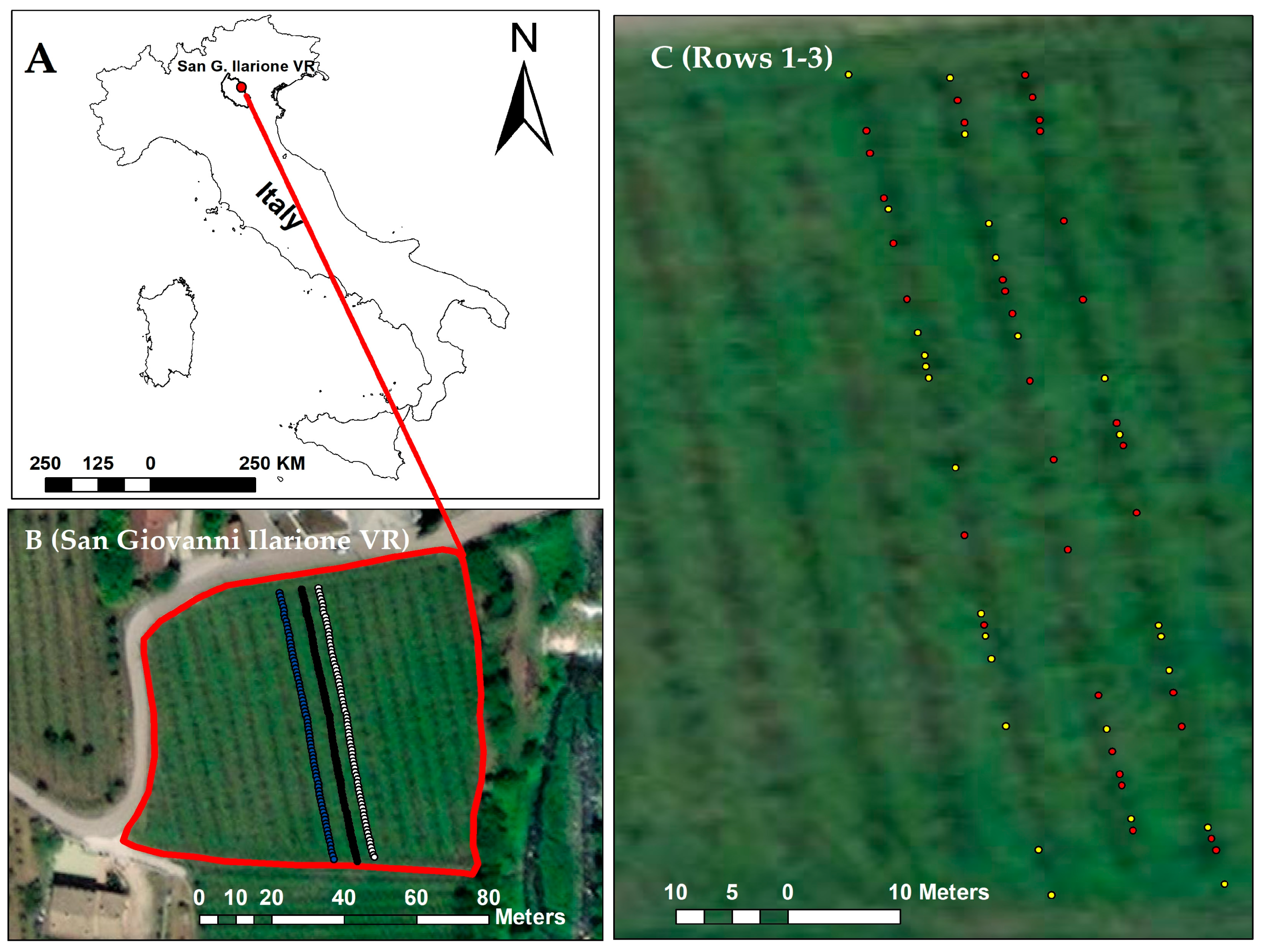
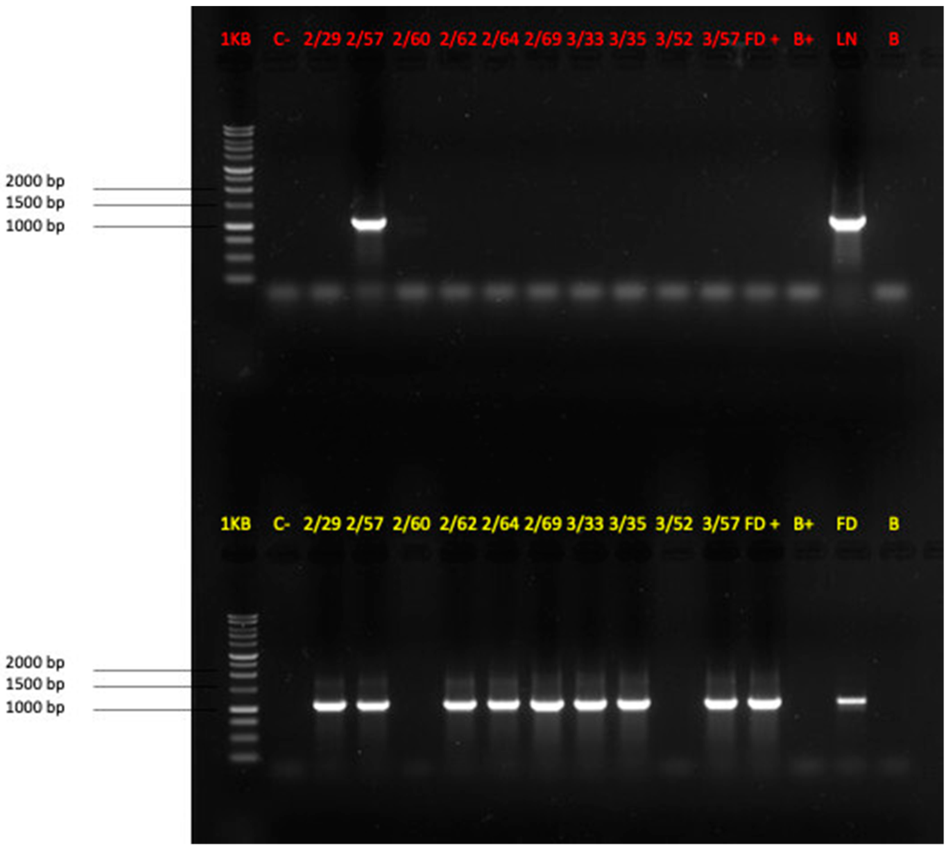
2.1. Leaf Sampling and Molecular Detection of Phytoplasmas

The actual presence or absence of phytoplasmas in grapevine tissues was checked by nested-PCR on 60 plants, 42 symptomatic and 18 asymptomatic. For each plant, 10 leaves with petioles were collected from the median sector of 3 different twigs, immediately refrigerated, and transferred to the laboratory. Petiole and midribs (1.5 g per sample, in 3 replicates) were separated from the lamina with a sterile razor blade and stored at −20°.

DNA extraction was performed by the CTAB method [24,25,26]. Briefly, midribs and petioles were ground with pestle and mortar in liquid nitrogen and the powder was transferred to a 1.5 mL plastic tube with 800 L of 3.5% ethyl–trimethyl–ammonium bromide in 1 M Tris–HCl pH8, 10 mM EDTA, 1.4 M NaCl (CTAB buffer). The mixture was then transferred into a 2 mL clean tube and centrifuged at 1000× g for 10 min. After the transfer of 1 mL of the suspension to a new tube, 2-marcaptoethanol was added to a final concentration of 0.2%), and tubes were incubated for 20 min at 65 °C. Then, an equal volume of chloroform: isoamyl alcohol (24:1) was added, followed by vortexing and centrifugation at 10,000× g for 10 min. The aqueous phase was separated, and nucleic acids were precipitated with an equal volume of cold isopropanol by centrifugation at 10,000× g for 15 min. The pellet was washed with 70% ethanol, dried, and dissolved in 100 L of nuclease-free water.

Nucleic acid concentration was determined with a Nanodrop (ThermoFisher Scientific, NJ, USA) and adjusted to 20 ng/μL. Purity was assessed by calculating the ratio of the absorbance at 260 nm over the absorbance at 280 nm and at 230 nm.

Detection of FDp or BNp was performed according to the EPPO guidelines for FD [25] by nested PCR, performing the first round of amplification with the generic P1/P7 primer couple [27]. The subsequent nested amplifications were carried out from the first diluted PCR products (1: 40) with specific primers, either for FD (R16(V)F1-R1) or for BN (R16(I)F1-R1) phytoplasmas [28]. Amplification products were run on 1% agarose gel in Tris-acetate-EDTA. The expected amplicon size was 1800 bp for the first amplification round and 1100 bp for both nested reactions. In parallel, controls of DNA extraction and positive and negative controls of the amplifications were also included in each round of experiments to exclude possible contaminations.

2.2. Spectral Data Collection

For spectral data acquisition, five spectral data campaigns were carried out at different growth stages from June to July 2022 (1st week: 8 June 2022, 2nd week: 15 June 2022, 3rd week: 21 June 2022, 4th week: 1 July 2022, and 5th week: 6 July 2022), when most of the plants in the vineyard were still asymptomatic for FD (

Table 1. Summary of spectral and PCR measurements.

Dates for Spectral Data Acquisition	Sensors	Vineyard Rows	No. of Samples	FD Positive Samples	FD Negative Samples
8, 15, 21 June, 1 and 6 July 2022	Hamamatsu (340–850 nm, 288 bands) and NIRScan sensor (900–1700 nm, 228 bands)	Row 1	20	07	13
		Row 2	20	13	07
		Row 3	20	13	07
		Total	60	33	27

). Two portable hyperspectral micro-spectrometers (Hamamatsu C12880MA series and DLP NIRScan Nano Evaluation Module (EVM), Texas Instruments, Dallas, TX, USA) were used to obtain spectral reflectance measurements of the leaf surfaces. Both spectrometers were handy and practical for field-level scanning due to their small size, portability, and comparatively lower unit cost. The Hamamatsu sensor record data with spectral sampling interval of about 2 nm and the spectral resolution is 15 nm (full width at half maximum), integrating 288 channels ranging from 340 nm to 850 nm. For the spectral data acquisition, the Hamamatsu sensor was mounted on a tripod (Figure 2A) to facilitate the collection from a nadir view. The Hamamatsu spectral data was acquired using an external cylindrical lens from a distance of approx. 0.3 m from the detached healthy and phytoplasma-infected grapevines’ leaf surface, resulting in an optical footprint diameter of about 5 cm within the leaf surface. The reflected light enters the device through a cylindrical lens and collimates the light before entering through slit. The Hamamatsu sensor was calibrated using a white reference (95% white reference panel), and we acquired for each date the radiance measurement of the white reference panel. The NIRScan sensor operates in the range of 900–1700 nm at 3.51 nm intervals with 228 spectral bands, and it is equipped with two integrated infrared lamps as a radiation source. The NIRScan acquisition was carried out using a software trigger in the reflectance mode and an average of 30 scans for each spectrum for each leaf of the selected plant. The NIRScan spectra was acquired using the factory-stored calibration data. The Hamamatsu sensor continuously records the data for approx. 10 s for which it acquired about 30 spectra while the NIRScan sensor recorded a set of 30 scans which means it is repeated 30 times a scan and outputs an average of 30 scans. All spectral measurements were acquitted on a sunny day from 10:00 to 14:00. For each date, three leaves were randomly picked up from each of the selected plants for spectra data acquisition.

2.3. Machine Learning Pipeline for Classification

The overall workflow for our research is graphically summarized in Figure 3. The spectral reflectance measurements acquired by two sensors Hamamatsu and NIRScan are exploited both separately and together (joined spectra) in order to make full use of the two wavelength ranges (340–1700 nm). To train the classifiers, spectral reflectance is fed to the classification algorithms (i.e., some opportune classification tools see Section 2.3.1) to attribute to each reflectance a binary label indicating whether it is positive or negative to FD (i.e., 1 = positive and 0 = negative to FD). The current study was conducted using a small set of samples (i.e., total plants: 60, FD positives: 33, and FD negative: 27). Thus, to evaluate the effectiveness of the proposed framework, we assess the performance of the trained models by using data that were not employed for the training phase (test samples) to obtain a non-biased estimation of its performance. In particular, we conduct the following: (1) We use the train-test split method in which the dataset is randomly divided into 70% training (FD positives: 22, and FD negative: 20) and 30% test (FD positives: 11, and FD negative: 7). However, as we have a small dataset, the train-test split method might be subject to high variance. To address this issue, we resort also to (2) leave-one-out (LOO) cross-validation, a special case of k-folds cross-validation, where k is equal to the size of our dataset (i.e., k = 60). We repeatedly divide the dataset using just one simple test set while we use the remaining ones as training sets. Afterwards, we calculate the average of their resulting performance, which minimizes the effect of random partitioning.

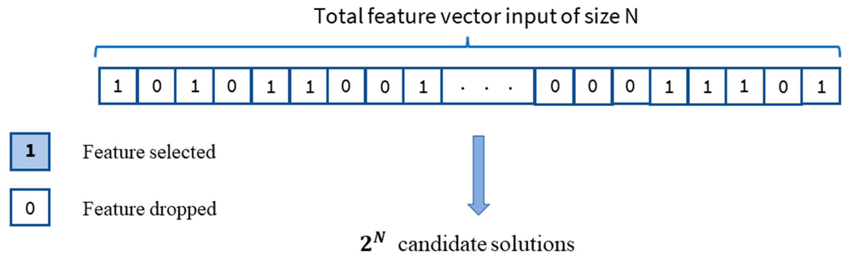
2.3.1. Feature Selection Algorithms

High dimensionality of the hyperspectral data is a critical factor that needs to be carefully considered when analyzing the hyperspectral data [17]. In this study, we propose two alternative techniques: (i) use the complete reflectance spectrum in order to exploit fully the information content of each band, and (ii) put forth a feature selection framework as a preprocessing tool that allows to reduce considerably the number of bands to be sent to the classification algorithms. In the second scenario, the feature selection framework is composed of two main steps: (1) an ensemble-based feature selection method (composed of sequential feature selector (SFS), feature importance score (FSI), recursive feature elimination (RFE)) are introduced to select a subset of feature bands containing the most significant features. This aims to eliminate the redundant and less relevant bands for the classification process. These three methods are a popular yet powerful feature selection paradigm due to their simplicity and effectiveness at appointing the most relevant features [29]. In this step, each feature selector provides a different subset of feature bands, which are simply aggregated by applying a majority-based vote mechanism. The bands with the most votes are chosen as the selected subset which will act as an accelerator for the successive step. (2) In the second step, the resulting subset of reduced bands with essential information content is subject to an intensive optimization search process using a proposed GA [30]. We exploit GA as a feature selection tool due to its customizability and it is characterized by its efficiency in exhaustively testing different sets of feature combinations [4]. Figure 3 illustrates an overview of the proposed framework.

Ensemble-Based Feature Selection

Selection score importance (SSI) has been introduced by Breiman [31] within random forest taking advantage of the so-called “split node function”. It selects a specific feature characteristic during the classification process to divide a tree at each training phase, thus, incorporating feature importance as one of its natural core functions [32,33]. Feature importance measures the significance of the feature to predict the target value. This technique is computed by summing the weighted impurity reductions of all nodes averaging them across the set of trees within the forest. As a consequence, features could be filtered based on this feature significance assessment. Sequential feature selector (SFS), on the other hand, compares the combinations of the different resulting feature subsets using a forward approach. In our case, we extracted the best-performing features subset exploiting the forward selection approach as in Kim et al. [29]. Recursive feature elimination (REF), similar to tree-based feature importance models, assigns recursively weights to the feature coefficients starting with the complete set of features by iteratively pruning the least important ones until reaching the targeted number of features [29]. For the sake of diversity, we have used two tree-based classifiers to assess the efficiency of the feature selected, the XGBoost classifier for SSI and the random forest classifier for REF and SFS. This way, we selected the 100 best features by using the ensemble method.

Genetic Algorithms (GA)

Inspired by the Darwinian, most fundamental evolution theorem ideas are the metaheuristic GA [30]. It was first developed as a search method modeled after the natural selection process of evolution, in which most suitable solutions are positively evolved through generations by means of operators like mutation, crossover, and selection. In this context, it has been utilized to further reduce the precedent selected subset of bands to extract the fittest individuals. In other words, the resulting subset of bands obtained by the first step ensemble selection methods (Figure 4) may have a range of spectral bands incorporating redundant and highly correlated feature bands which can be eliminated. Thus, we are searching for the least relevant bands that could be dropped without impacting much our classification accuracy performance.

The GA method starts by randomly creating an initial collection of population chromosomes (i.e., p = 20) that serve as potential solutions to our optimization task. A chromosome stands for a resolution of a binary array of size N (i.e, N = 100), representing the spectral input wavelength bands (a subset of selected features) where 1 denotes the feature band is picked and 0 it is dropped. As a result, the first population has initial potential solutions with population $P$ of size $M$ from a $2^N$ possible chromosome feature subset. In the following stage, the quality of each chromosome (solution) in the generated initial population is assessed using a selection operation based on an objective function. Natural selection then starts its generational process generating the set of chromosomes allowed to reproduce and become parents and pass their genes. The crossover procedure is then used to recombine the data from the two parents chosen in the previous phase to create new progenies. It chooses a random cut point and accomplishes the combination between two chromosomes by mixing them for the new population.

Another genetic operation used to increase population variety is the mutation operation, which modifies the genetic make-up of parents depending on a mutation rate. A random gene band is chosen from an arbitrary selected chromosome in the new population, and its value is changed from 0 to 1 or vice versa (Figure 5). The purpose of mutation is to avoid the algorithm settling on a local minimum. This process is repeated up until the termination criteria is met, then the convergence is reached, producing a final subset of the fittest feature set of bands over all produced generations.

Let X be our feature spectral input (i.e., training set) defined as follows:

$$X=\{x_i\in X|i=1,\dots ,N\}$$

(1)

where $x_i$ is a single feature vector sample from the $i^{th}$ position with size N, given that N is the total number of spectra feature bends. Let P be its corresponding binary set with size $2^N\ast N$, where $2^N$ is the combination of all possible features subset to represent our GA chromosome pool.

The underlying idea behind the proposed method is to select the best subset of feature bands maximizing or at least roughly maintaining the accuracy at the same level compared to when exploiting the whole spectra. Thus, the constraint of our GA objective function would be a trade-off between the classification accuracy and the size of feature subset X. Al-Saddik et al. [4] exploited GA to investigate the optimal spectral bands to be selected for FD. However, GA can be pushed further by customizing its cost function to reduce considerably the resulting subset of features by formulating it, adding a constraint trade-off between the accuracy performance and the size subset of features.

The objective function to assess each potential solution chromosome is defined as follows:

$$Fitness function=max {\displaystyle \sum }_{j=1}^M{\displaystyle \sum }_{k=0}^{T-1}f \left(P_k^j\right) \mathrm{such}\mathrm{that} P_k^j\in P_k \mathrm{given}\mathrm{that} j\in \{1,\dots ,\mathrm{M}\}$$

(2)

where M is the population size and k is the generation tournament $k \in \{0,\dots ,\mathrm{T}-1\}$. T is the maximum number of generations used as a stop criterion for our GA.

We define $f(P_k^j)$ as follows Alba et al. [34]:

$$f\left(P_k^j\right)=\left(\alpha \ast \left(1-Ac{c}_k^j\right)+\left(1-\alpha \right)\ast \left(1-\left(x_k^j.nbrFeatures\right)/N\right)\right)\mathrm{given}\mathrm{that}0 \le \alpha \le 1$$

(3)

where Acc is the classifier performance accuracy on the $X_k^j$ which is the data feature subset selected by the chromosome individual computed as follows:

$$X_k^j=X \ast P_k^j$$

(4)

with $X_k^j.nbrFeatures$ as being its size (i.e., the sum of genes selected within the $P_k^j$ chromosome set to 1); the constant is used as weight to leverage between the accuracy performance and the subset of size of features. In our case, it has been fixed to 0.1. It works as a penalization factor to the chromosomes with high number of genes (i.e., when two chromosomes have a similar accuracy, it favors the ones with less features). The pseudo code algorithm below (

Table 2. Genetic Algorithms (GA) for feature selection.

Genetic Algorithm for Feature Selction

//Initialize variables $k=0$, NbrTotalFeatures = 100, stop_criterion = False, α= 0.1, MaxNbrGeneration = 4000, N = TotalNumberOfGenes, $M$ = NbrOfPopulation // Initialize a number of ${\mathit{P}}_{\mathit{k}}$ binary chromosomes with random binary values of genes 1.Generate initial population ${\mathit{P}}_{\mathit{k}\mathbf{=}\mathbf{0}}$  While (stop_criterion ≠ True) { //compute the score of each chromosome in the population using fitness function 2.Evaluation //Evaluate ${\mathrm{P}}_{\mathrm{k}}$ the binary population chromosomes chosen genes For $P_k^j$∈ $P_k$ given that $j\in${1,.., $M$} // For each binary chromosome in Population {        // transoform the binary chosen chromoroses to the classification feature space        $X_k^j$=Train_features* $P_k^j$        // train classification model using 3-fold cross-validation        ${\mathit{accuracy}}_k^j$ = Train_model($X_k^j$)        //compute score function        $X_k^j$.nbrFeatures = Sum($P_k^j$)        ${\mathit{score}}_K^j$= f ($P_k^j$, $X_k^j$.nbrFeatures, α, N) Equation (3) } end For 3. generate the progeny generation { //select the chromosomes allowed to reproduce the next generation based on the fitness function scores I. Selection //recombine chromosomes to choose which genes are transferred from parents to new progeny II. Crossover //random inversion in the selection progeny binary genes III. Mutation } 4. update $P_k$ with the new progeny generation k=k+1 // increment the generation tournament If (k >= MaxNbrGeneration) then { stop criterion ==True} } end While

) illustrates the related GA framework pseudo code.

2.3.2. Classification Models

Among the variety of existing machine learning classifiers, we have chosen five different linear and non-linear binary classification approaches for their potential in this application domain and to determine which one is most effective at recognizing FD disease, namely, simple logistic regression (LR), support vector machines (SVMs), gradient boosting (XGBoost), random forest (RF), and Cubist regression (Cubist) classifiers.

• Logistic regression (LR): The LR classifier is a simple yet effective technique that takes advantage of logistic function to model dependent variables that are linearly related to the log odds for binary classification problems. After ranking the features in terms of relevance, the model can be employed to forecast the probability of the classes based on its input features [35]. For the purpose of describing the phenomenon of classification, it is useful to tie the likelihood of a class to a group of explanatory features. In order to avoid overfit, the “L2” penalty is exploited in addition to the “C” value hyperparameter governing the degree of regularization. LR is widely employed for binary classification tasks in the remote sensing community due to its simplicity, parallelizability, and high interpretability producing extremely competitive results [36].
• Support vector machines (SVMs): SVMs are known to be one of the most promising classification tools as they are widely used within the remote sensing community different classification and regression tasks [37,38,39]. Its main objective is to find an optimal hyperplane that separates a given dataset. Moreover, to cope with nonlinear patterns, an SVM kernel function aims at mapping the original data into a higher new dimensional space in which finding an optimal separation hyperplane between data becomes linearly feasible in the new transformed space. In our case, the radial basis function (RBF) has been exploited as an SVMs kernel. RBF function is widely used within the machine learning community, due to its flexibility, and similarity to the Gaussian distribution, it can overcome the feature space complexity. We put forth the SVMs classifier in this work motivated by their highly efficient performance in hyperdimensional classification tasks.
• Random forest classifier (RF): A decision tree is a supervised learning method based on a set of rules arranged in the shape of a tree for solving both classification and regression problems [31]. RF, as its name suggests, is an extension of the single decision tree yet better suited for a complex dataset. In order to cope with decision tree overfitting limitations, it takes advantage of exploiting averaging on a bunch of decision trees during the training phase. In doing so, it is possible to solve the problem with improved generalization.
• Gradient boosting classifier (XGBoost): Due to its high effectiveness and accuracy, extreme gradient boosting is one of the most used machine learning techniques. Similar to RF, it combines different machine learning algorithms to create a strong predictive classifier [40]. In contrast to gradient boosting decision trees, which is based on the gradient-powered decision trees exploiting linear combination of an ensemble of weak learning models where the trees are produced sequentially, correcting the error of prior weak learners, XGBoost builds its trees in parallel elevating its performance considerably with high computational speed. Chen and Guestrin [41], for this latter reason, chose XGBoost as the GA iterative optimization fitness assessment classifier.
• Cubist regression models (CB): Another model based on decision trees is the Cubist rule-based model [cubist]. A potent algorithm developing sequentially a series of trees. It induces accurate yet simple rules built and selected repeatedly at each iteration. Unlike RF, CB returns a set of rules linked to sets of multivariate models rather than a single final model. Then, depending on the rule that best matches the predictors, a particular collection of predictor variables will choose an actual prediction model [42,43]. To some extent, in order to interpret the complicated links between the influential features the Cubist model was seen to be very promising compared to tree methods counterparts [44].
• Trees-based models can produce a more thorough predictive accuracy when compared to traditional linear machine learning techniques. Their main benefits for classification tasks include (a) a reduced risk of overfitting, (b) a small number of effective tuning hyperparameters, (c) the ability to automatically determine variable importance in order to interpret the variable contribution mechanism in the final prediction model. To recapitulate, in order to capture the linear/non-linear relationships between the VIS-NIR hyperspectral bands, various predictors, random forests, Cubist and XGBoost-based tree ensemble models in addition to LR and SVMs algorithms are used in this context. A 3-fold cross-validation set has been exploited during the training process searching for the best hyper-parameters values of our respective supervised learning models. We use Savitzky–Golay filter (SG), a polynomial interpolation, for smoothing the input data as a pre-processing step with a polynomial order 2, and a passing window equal to 13. The K-fold cross-validation resulting scores in the training stage use the forward selection as in Kim et al. [29].

2.4. Classification Accuracy Assessment

To evaluate the performance of classifiers, several evaluation measures such as accuracy, precision, recall, and F1-score were used. The accuracy metrics formula is shown in the equations below.

$$Accuracy=\frac{TP+TN}{TP+FN+TN+FP}$$

(5)

$$Precision=\frac{TP}{TP+FP}$$

(6)

$$Recall=\frac{TP}{TP+FN}$$

(7)

$$F1 Score=\frac{2 \ast \left(Recall \ast Precision\right)}{\left(Recall+Precision\right)}$$

(8)

where TP is a true positive which indicates the sample that is diseased and also predicted as diseased by the model. TN is true negative which indicates the sample that is healthy and also predicted as healthy by the model. FP is false positive which indicates the sample that is originally healthy but predicted as diseased by the model. Meanwhile, FN is false negative which indicates the sample that is originally diseased but predicted as healthy by the model. In the results section, we reported accuracy metrics (Tables 3–5) and in the discussion section (Tables 6 and 7) we report all metrics for the best achieved results. All the statistical analyses were carried out using python.

3. Results

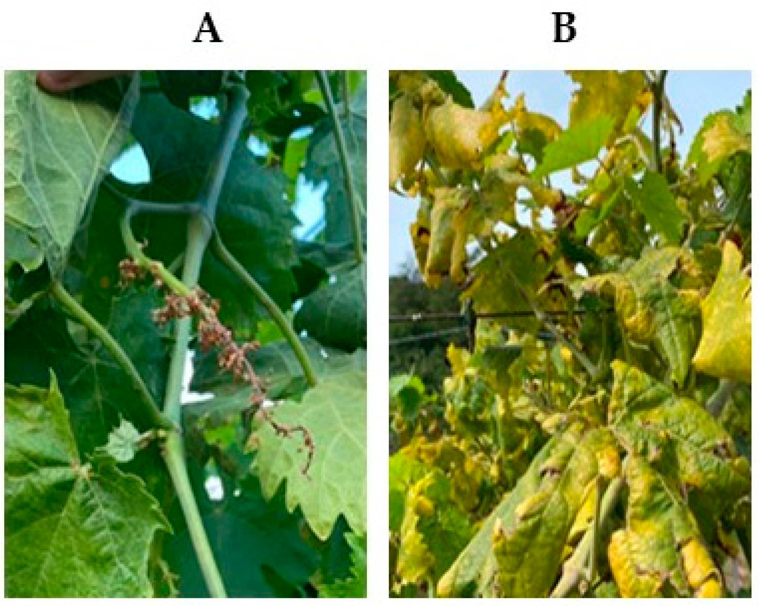
3.1. Visual Inspection of the Vineyard and Molecular Detection of FD and BN Phytoplasmas

The visual inspection carried out on four different dates revealed symptoms that possibly referred to phytoplasmas in about 30% of all the 228 plants (Figure 6).

Figure 7 shows the results of a representative experiment. Molecular tests confirmed symptom-based predictions only in 60% of cases with no bias towards infected or non-infected plants. In detail, 26 of 42 symptomatic plants tested positive for FD or BN, while 11 of 18 plants with no apparent phytoplasmatic symptoms actually tested negative. Only one plant (symptomatic) tested positive for both pathogens. These results were used to label the plants as “healthy” or “diseased”.

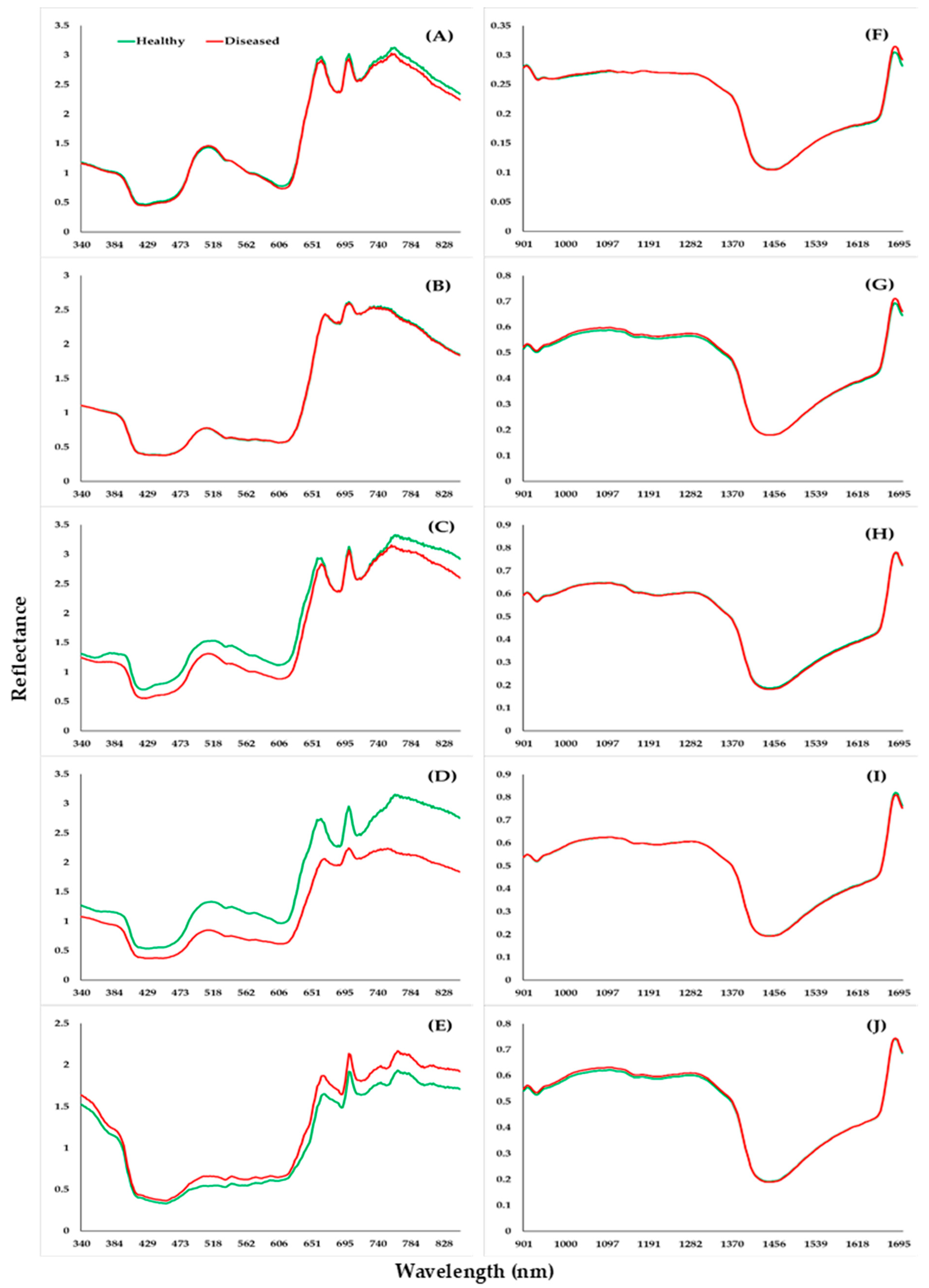
3.2. Healthy and Diseased Plants to Spectra

To compare the reflectance of healthy and diseased plants, the average reflectance of all healthy and diseased plants from both sensors are presented in Figure 8. The difference in the reflectance of healthy and diseased are observed, and it can be seen that the reflectance of the Hamamatsu sensor shows high differences between healthy and diseased while the reflectance from the NIRScan sensor has small differences in the spectra. In the early growth stages, the differences between healthy and diseased Hamamatsu spectra are small but they get higher for the later stage. For the first and second weeks, both groups show similar values; but, in the second and third weeks, higher reflectance is observed in VIS-NIR spectral region (400–850 nm) for healthy plants compared to diseased plants, while in the fourth week an opposite pattern is observed. On the other hand, both plant groups did not show any big differences in spectra acquired by the Texas instrument, and almost for all growth stages, both groups show similar reflectance values. Only a small difference in spectra is observed in the spectral range of 900–1300 nm in the second and fifth week of the data acquisition but for other dates, the spectra of both groups almost show similar values.

3.3. Classification Performance

The model for the vineyard health classification to the classes of “Healthy” as FD-negative, and “Diseased” as FD-positive was trained using different classifiers (LR, SVMs, XGBoost, RF, and Cubist) and reported the best models’ accuracies at each growth stage in

Table 3. Classification accuracies (%) using all bands, ensemble-based reduced features, and features reduced by genetic algorithms (GA) technique of both sensors (Hamamatsu and NIRScan) on test samples. In the column “Feature selected by GA method” the values outside and inside the brackets correspond to accuracy (%) and features selected by GA, respectively.

Dates	Hamamatsu			NIRScan
	All Bands (288)	Features (100) Selected by Ensemble Method	Features Selected by GA Method	All Bands (228)	Features (100) Selected by Ensemble Method	Features Selected by GA Method
8 June 2022	67	72	61 (6)	61	61	61 (10)
15 June 2022	67	72	78 (9)	61	67	61 (8)
21 June 2022	72	78	61 (13)	72	67	72 (6)
1 July 2022	89	78	89 (13)	61	61	61 (10)
6 July 2022	61	61	61 (12)	61	67	72 (7)

,

Table 4. Classification accuracies (%) using all bands, ensemble-based reduced features, and features reduced by the genetic algorithms (GA) technique of both sensors (Hamamatsu and NIRScan) with leave-one-out (LOO) cross-validation on the whole dataset. In the column “Feature selected by GA method” the values outside and inside the brackets correspond to accuracy (%) and features selected by GA, respectively.

Dates	Hamamatsu			NIRScan
	All Bands (288)	Features (100) Selected by Ensemble Method	Features Selected by GA Method	All Bands (228)	Features (100) Selected by Ensemble Method	Features Selected by GA Method
8 June 2022	62	63	55 (10)	58	57	55 (8)
15 June 2022	62	85	63 (7)	43	45	48 (18)
21 June 2022	58	58	62 (8)	60	62	63 (11)
1 July 2022	72	77	72 (8)	60	57	68 (3)
6 July 2022	55	55	60 (7)	55	55	63 (12)

and

Table 5. Classification accuracies (%) using all bands of both sensors (Hamamatsu and NIRScan joined), features selection by the ensemble method, then by the genetic algorithms (GA) technique of both sensors (joined spectra) on test samples and leave-one-out (LOO) cross-validation on the whole dataset. In the column “Feature selected by GA method” the values outside and inside the brackets correspond to accuracy (%) and features selected by GA, respectively.

Dates	Test Samples Accuracy			Test Samples Accuracy
	All Bands (516)	Features (100) Selected by Ensemble Method	Features Selected by GA Method	All Bands(516)	Features (100) Selected by Ensemble Method	Features Selected by GA Method
8 June 2022	61	67	67 (9)	58	55	60 (14)
15 June 2022	61	61	61 (8)	55	58	60 (12)
21 June 2022	67	61	72 (8)	55	57	58 (15)
1 July 2022	72	67	83 (7)	72	77	72 (20)
6 July 2022	67	67	72 (8)	57	58	62 (20)

. In the first scenario, the models were trained using the training set and assessed the performance using test samples while in the second scenario, the models were trained using the whole dataset and assessed the performance using the LOO cross-validation method. Table 3 shows the classification results of the test set for both sensors using all bands, reduced by the ensemble method, and then finally using GA. The results of the Hamamatsu sensor are reported in Table 3 where we can see that when all bands were considered the accuracy ranges from 61% to 89% while for the NIRScan sensor it ranges from 61% to 72%. The Hamamatsu sensor shows better accuracy than the NIRScan sensor except in the third week (21 June 2022) when the NIRScan showed the same accuracy of 72%. The highest accuracy is achieved in the fourth week (1 July 2022) for the Hamamatsu sensor when all the bands were used. The classification accuracy pattern of both sensors is with respect to growth stages; the highest accuracy is achieved in the fourth week where Hamamatsu all bands give an accuracy of 89% and NIRScan gives 72% in the third week, but a drop in accuracy is observed where on the fifth week both sensors achieved 61% accuracy to classify healthy diseased plants.

The results based on the Hamamatsu-reduced data by the ensemble method show that the accuracy ranges from 61% to 78% while, for the data further reduced by GA, the accuracy ranges from 61% to 89%. The highest accuracy is achieved using features 13 extracted by GA on the fourth week and suggests that spectral bands (374, 392, 395, 416, 479, 534, 622, 654, 683, 692, 713, 756, 798 nm) had the potential to discriminate between healthy and phytoplasma-infected leaves. On the other hand, the NIRScan sensor shows slightly lower accuracy compared to the Hamamatsu sensor where the highest accuracy achieved is 72% by using GA-extracted features on the third and fifth weeks. The key spectral bands (third week: 901, 1108, 1367, 1440, 1456, 1462 nm; fifth week: 905, 933, 989, 1394, 1398, 1476, 1691 nm) were extracted by using the GA method for NIRScan sensor, which shows the potential to discriminate between healthy and phytoplasma-infected leaves with an accuracy of 72%.

This study is based on small training samples. The classification accuracy between healthy and diseased leaves also analyzed using LOO cross-validation on the whole dataset and results are summarized in Table 4. When all bands of the Hamamatsu sensor were undertaken, the accuracy values vary between 55% to 72% while for the NIRScan sensor they vary from 43% to 60%. Similar to results based on the training set, the results of LOO cross-validation also show that the Hamamatsu sensor gave slightly better accuracy with 85% accuracy in the second week compared to the NIRScan sensor, where a maximum of 68% accuracy is achieved in the fourth week. Among the two feature selection techniques for the Hamamatsu sensor, the features extracted by the ensemble methods perform slightly better than GA while for the NIRScan sensor, GA is performing better with an accuracy of 68% in the fourth week (1 July 2022).

To exploit the full range of spectra (340–1700 nm) by joining spectra of two sensors, the classification results between healthy and diseased leaves were analyzed. Table 5 shows the classification results using all bands, reduced by the ensemble method, and finally, GA and models were assessed by using the test samples and LOO cross-validation on all samples. For the classification results using all bands of joined spectra of test samples, the accuracy ranges from 61% to 72%, while for the reduced bands extracted by the ensemble and GA methods, the accuracy ranges from 61% to 67% and from 61% to 83%, respectively. The seven features extracted by GA show better accuracy with a maximum of 83% in the fourth week (1 July 2022) compared to the features extracted by the ensemble method where a maximum accuracy of 67% is achieved and even using all bands where the maximum accuracy of 72% is achieved in 4th week (1 July 2022). When the models were assessed by using LOO cross-validation considering all samples, the classification results show slightly lower accuracy compared to results achieved on test samples where the highest accuracy of 77% is achieved by using features extracted by the ensemble method in the fourth week. On the other hand, when all bands of joined spectra were undertaken and models were assessed by LOO cross-validation, the maximum accuracy is achieved up to 72% on the fourth week, while the same accuracy of 72% is achieved in the fourth week using the 20 features extracted by GA.

3.4. Confusion MATRIX

From the confusion matrix of results of 18 test samples (Figure 9A), it can be seen that out of 11 plants suffering from the FD infestation, all are classified correctly, whereas two healthy plants are classified to the class “Diseased” wrongly as “False positive” out of the seven healthy plants. Considering the results of LOO cross-validation on the whole dataset of 60 samples (Figure 9B), 29 are correctly classified to the class “Diseased”, whereas four diseased plants are misclassified as “False negatives”. On the other hand, out of 27 healthy plants, 22 are identified correctly, whereas five plants are misclassified as “False positives”.

4. Discussion

The vineyard selected in this study, planted in 2005, was in generally poor phytosanitary conditions, with disetaneous vines, due to multiple replacements of old/dead plants along the years (26% of plants less than 5 years old, 20% more than 15 years, about half of the plants between 5 and 15 years old). The vineyard was affected by several chronic diseases, especially trunk dieback and viral infections, while seasonal epidemics were correctly controlled by regular pesticide treatments. This general situation, plus an exceptionally dry and hot season, complicated the visual inspection of symptoms, which correctly identified phytoplasma-infected vines in 60% of plants, in line with variability of previously reported surveys [22]. Overall, the experimental plot posed a serious challenge for the reflectance-based prediction of actual phytoplasma infection.

The spectral properties of the leaf change when the cellular leaf structure and physiology are altered due to the presence of a pathogen (i.e., FD, BN) which causes metabolic and pigment changes resulting in altered leaf spectral properties of healthy and diseased leaves. Based on the similar pathogenetic process of FD and BN diseases, it is not expected that reflectance data may differ between the two. Symptoms of phytoplasma infection due to FDp or BNp are indistinguishable and are related to the peculiar physiological alterations consequent to the activity of phytoplasmas’ effectors into the plant phloems [45,46]. Such changes include the accumulation of soluble carbohydrates with feedback inhibition of photosynthesis and of secondary metabolites involved in the shikimic acid and oxidative pentose phosphate pathways, together with induction of plant defense reactions and alteration of plant hormonal balance [47,48]. Similar to Al-Saddik et al. [4] and Naidu et al. [11], some evident differences in leaf reflectance between healthy and diseased grapevines were identified. However, higher differences were observed in the reflectances in the Hamamatsu spectra compared to the NIRScan spectra. The reflectance of the Hamamatsu sensor showed small differences between healthy and diseased leaves in the early vegetative growth stages while stronger differences were observed in the later stage (third and fourth week). Higher differences in the reflectance in the VIS spectral region are due to a decrease in pigment concentrations of the infected leaves. Hence, infected leaves absorb less light and reflect more to the sensor [49,50,51]. The differences in the Hamamatsu spectra of both groups reveal that in the infected leaves pigment concentration started to reduce in early growth stages even though the leaves had not yet displayed discoloration or yellowing, and this indeed is an indication of the infection in the leaf.

The best classification accuracies out of five different classifiers (LR, SVMs, XGBoost, RF, and Cubist) to discriminate between asymptomatic healthy and diseased spectra are summarized in Table 3, Table 4 and Table 5 where the results indicate that the detection of phytoplasma-infected leaves is possible with hyperspectral sensors. Higher classification accuracies are achieved with a maximum of 89% with Hamamatsu data in the fourth week, while the NIRScan sensor shows slightly low accuracies with a maximum of 72% (Table 3). The differences in classification accuracies of the two sensors are due to the reflectance differences between healthy and diseased leaves of each sensor as in the case of the Hamamatsu sensor, where the reflectance of healthy and infected leaves show higher differences compared to the NIRScan sensor. When comparing the results of test samples (30% samples) and LOO cross-validation on the whole dataset, the test samples accuracy yielded slightly higher classification accuracies compared to the accuracies achieved by LOO cross-validation on the whole dataset. The train-test split approach estimates the performance of a model trained on a subset of the whole dataset which could bias the model’s true performance. On the other hand, the LOO cross-validation is approximately unbiased because the difference in size between the training set used in each fold and the entire dataset is only a single pattern [52]. Classification accuracies were analyzed using complete spectra and also using the reduced spectral bands extracted by feature selection algorithms (Ensemble and GA). Feature selection is commonly used in the pre-processing of hyperspectral data to exclude irrelevant or less important features which helped to improve the performance of the model and also reduce the computational cost of modeling [19]. Higher classification accuracies were observed when the Hamamatsu sensor was used compared to the NIRScan sensor. By applying feature selection techniques, the feature set was reduced and using selected features we achieved comparable or even slightly better accuracies compared to those achieved when no feature selection is applied. The results of this study show the effectiveness of using the feature selection algorithm and overall better accuracies are achieved when reduced data was used to discriminate between healthy and diseased leaf spectra. The 13 key spectral bands of the Hamamatsu sensor extracted by GA are reported to be 374, 392, 395, 416, 479, 534, 622, 654, 683, 692, 713, 756, and 798 nm, which differentiate healthy and infected grapevine leaves with an accuracy of 89% (precision of 85%, recall of 100%, and F1 score of 92%,

Table 6. Summary of best accuracies achieved on test samples, full spectra, ensemble method (Ens method), and genetic algorithms (GA).

Dates	Sensors	Features	Classifiers	Accuracy (%)	Recall (%)	Precision (%)	F1 Score (%)
1 July 2022	Hamamatsu	GA (13)	LR	89	100	85	92
21 June 2022	NIRScan	GA (7)	RF	72	91	71	80
1 July 2022	Joined spectra	GA (7)	SVM, LR	83	91	83	87

) with LR classifier by using test samples. On the other hand, in case of the NIRScan sensor, the maximum accuracy of 72% (precision of 71%, recall of 91%, and F1 score of 80%, Table 6) was achieved on the test samples with RF classifier using the reduced bands extracted by GA were 905, 933, 989, 1394, 1398, 1476, and 1691 nm. As the current study is based on a small sample size, to avoid overestimating the true accuracy, the classification results were also analyzed using LOO cross-validation. The best accuracies achieved from LOO cross-validation on the whole dataset are summarized in

Table 7. Summary of best accuracies achieved on whole dataset with leave-one-out (LOO) cross-validation, full spectra, ensemble method (Ens method), and genetic algorithms (GA).

Dates	Sensors	Features	Classifiers	Accuracy (%)	Recall (%)	Precision (%)	F1 Score (%)
1 July 2022	Hamamatsu	Ens method (100)	SVM	85	88	85	87
21 June 2022	NIRScan	GA (3)	GB	68	88	66	75
1 July 2022	Joined spectra	Ens method (100)	RF	77	74	88	81

. The highest accuracy of 85% (precision of 85%, recall of 88%, and F1 score of 87%, Table 7) was achieved for the Hamamatsu sensor by using SVM classifiers trained by 100 spectral bands selected by the ensemble method. The selected 100 features were mainly (71% features) from the VIS spectral range (400–700 nm), 27% of the selected features were from the ultraviolet region, and only 2% of the features were from the NIR spectral region. In case of the NIRScan sensor, low accuracy of 68% (precision of 66%, recall of 88%, and F1 score of 75%, Table 7) was achieved by using GB classifiers trained by three spectral bands (937, 996, 1592 nm) selected by the ensemble method. Spectral regions similar to the ones identified in our study were also reported in other studies where authors used the spectral data to predict the classification of healthy grapevines and phytoplasma-infected ones, showing yellowing and leaf-roll symptoms, very similar to those of phytoplasma infections [5].

The spectral bands in the VIS-NIR range (400–840 nm) are considered critical to identify reflectance differences in leaves subjected to biotic stressors because reflectance in blue and red regions is sensitive to leaf pigment content (chlorophyll, carotenes, and xanthophyll) and might be an indicator of the plant health status [13,53]. These differences allowed several authors to successfully employ these methods for detecting biotic and abiotic stresses in grapevines [4,5,22]. However, the pattern of differences between the spectra of the two groups vanished when the NIRScan spectra were observed; this might be due to the fact that the physiological changes in relation to a reduction of leaf water content do not vary during the early stage of infection. Further, it is hard to tell if the spectral differences between healthy and diseased leaves will increase with the increase in infection throughout the vegetative growth stages. In fact, the grapevine leaves responded in different manners in the later growth stages. The third and fourth-week healthy leaves showed higher reflectance values for the Hamamatsu sensor; but, a week later, in the fifth week, the opposite pattern was observed in the spectra most likely due to other symptoms from other several chronic diseases that can affect the spectral data. Somewhat similar alterations affecting chlorophyll content and different pathways in the secondary metabolism are also found in response to other biotic and abiotic stressors, such as virus-like symptoms, esca dieback, or drought stress. However, more detailed analyses of different diseases may reveal peculiar metabolic changes possibly associated with reflectance differences and deserve further investigation [54,55,56]. In fact, comparative reports are lacking about the physiological alterations caused by different stressors on the same variety, in a time course along the growing season and the disease progression. The results of this study suggest that even in a complex phytopathological scenario, the reflectance within the VIS-NIR spectral range is very promising to detect phytoplasma-infected plants. The confusion matrix (Figure 9) shows the overall scenario of the best classifier (LR) where we can observe that from the 13 infected none are resulting as “False negatives” and two samples (11.11%) are classified as “False positives” when using the test sample (18 samples). In case of LOO cross-validation, out of 60 samples, only 4 samples (6.67%) were wrongly classified as “False negatives” and 5 samples (8.33%) were classified as “False positive”. In fact, from the analysis of the confusion matrix, it is more beneficial for the end-user farmers to have fewer “False negatives” with respect to “False positives”. This allows the identification of the source of the FD outbreak that might affect the healthy plants, thus providing higher chances to prevent disease spread in neighboring vineyards.

The present study is based on a small dataset and conducted on a single grapevine variety. The further validation of our results will require the collection of a larger dataset (especially from asymptomatic samples) from commercial vineyards in other growing seasons and other varieties. A practical and efficient application would rely on the integration of such low-cost hyperspectral sensors with ground vehicles that can collect data while performing other agricultural practices (i.e., spraying, trimming, etc.). Such application will be extremely useful to vine growers to scout for infected vines over a larger acreage in a relatively small time-frame.

5. Conclusions

This study evaluated the field applicability of low-cost portable VIS-NIR and NIR spectrometers for detecting FD symptoms in a cv. A Garganega vineyard was cultivated by using all bands and reduced features in the range of 350–840 and 900–1700 nm. Five field surveys were carried out to acquire the spectral data at different growing stages to identify the best suitable time to identify FD-associated signals in reflectance data. Five different classifiers were used to identify the healthy and diseased groups by using all bands in addition to the extracted features by ensemble and GA methods. The results of the study suggest that spectral wavelengths have discriminatory power to differentiate the healthy from the infected vines. The critical bands are found in the spectral range of 374, 392, 395, 416, 479, 534, 622, 654, 683, 692, 713, 756, and 798 nm, and were associated with symptomatic as well as asymptomatic samples. Moreover, such common wavelengths could differentiate healthy and phytoplasma-infected leaves throughout the different phenological stages of grapevines across the growing seasons. The GA-based features classification accuracies were significantly higher than those obtained with all bands. Overall, the proposed low-cost optical sensors in the VIS-NIR domain were found suitable under field conditions for non-destructive phytoplasma detection in grapevines, at an early stage when the disease symptoms are not visible on the leaves. Future studies will be needed to collect more spectral data from phytoplasma-infected and healthy leaf samples of other grapevine varieties in order to consolidate the results reported in the present study and extend their validity. Moreover, additional studies on different biotic and abiotic stressors using the same approach would be of utmost importance to address the crucial issue of remote sensing specificity in plant disease diagnosi.

References

1. Jeger, M.; Bragard, C.; Caffier, D.; Candresse, T.; Chatzivassiliou, E.; Dehnen-Schmutz, K.; Gilioli, G.; Jaques Miret, J.A.; MacLeod, A.; Navajas Navarro, M.; et al. Risk to Plant Health of Flavescence Dorée for the EU Territory. EFSA J. 2016, 14, e04603. [Google Scholar] [CrossRef]
2. Ripamonti, M.; Pegoraro, M.; Rossi, M.; Bodino, N.; Beal, D.; Panero, L.; Marzachì, C.; Bosco, D. Prevalence of Flavescence Dorée Phytoplasma-Infected Scaphoideus Titanus in Different Vineyard Agroecosystems of Northwestern Italy. Insects 2020, 11, 301. [Google Scholar] [CrossRef] [PubMed]
3. Martini, M.; Pavan, F.; Bianchi, G.L.; Loi, N.; Ermacora, P. Recent Spread of the “Flavescence Dorée” Disease in North-Eastern Italy. Phyt. Moll. 2019, 9, 207. [Google Scholar] [CrossRef]
4. Al-Saddik, H.; Simon, J.C.; Cointault, F. Assessment of the Optimal Spectral Bands for Designing a Sensor for Vineyard Disease Detection: The Case of ‘Flavescence Dorée. Precis. Agric. 2019, 20, 398–422. [Google Scholar] [CrossRef]
5. Sinha, R.; Khot, L.R.; Rathnayake, A.P.; Gao, Z.; Naidu, R.A. Visible-near Infrared Spectroradiometry-Based Detection of Grapevine Leafroll-Associated Virus 3 in a Red-Fruited Wine Grape Cultivar. Comput. Electron. Agric. 2019, 162, 165–173. [Google Scholar] [CrossRef]
6. Musci, M.A.; Persello, C.; Lingua, A.M. Uav Images and Deep-Learning Algorithms for Detecting Flavescence Doree Disease in Grapevine Orchards. Int. Arch. Photogramm. Remote Sens. Spat. Inf. Sci. 2020, 43, 1483–1489. [Google Scholar] [CrossRef]
7. Tessitori, M.; La Rosa, R.; Marzachì, C. Flavescence Dorée and Bois Noir Diseases of Grapevine Are Evolving Pathosystems. Plant Health Prog. 2018, 19, 136–138. [Google Scholar] [CrossRef]
8. Wei, X.; Johnson, M.A.; Langston, D.B.; Mehl, H.L.; Li, S. Identifying Optimal Wavelengths as Disease Signatures Using Hyperspectral Sensor and Machine Learning. Remote Sens. 2021, 13, 2833. [Google Scholar] [CrossRef]
9. Calamita, F.; Imran, H.A.; Vescovo, L.; Mekhalfi, M.L.; La Porta, N. Early Identification of Root Rot Disease by Using Hyperspectral Reflectance: The Case of Pathosystem Grapevine/Armillaria. Remote Sens. 2021, 13, 2436. [Google Scholar] [CrossRef]
10. Mahlein, A.-K.; Kuska, M.T.; Behmann, J.; Polder, G.; Walter, A. Hyperspectral Sensors and Imaging Technologies in Phytopathology: State of the Art. Annu. Rev. Phytopathol. 2018, 56, 535–558. [Google Scholar] [CrossRef]
11. Naidu, R.A.; Perry, E.M.; Pierce, F.J.; Mekuria, T. The Potential of Spectral Reflectance Technique for the Detection of Grapevine Leafroll-Associated Virus-3 in Two Red-Berried Wine Grape Cultivars. Comput. Electron. Agric. 2009, 66, 38–45. [Google Scholar] [CrossRef]
12. Gao, L.; Wang, X.; Johnson, B.A.; Tian, Q.; Wang, Y.; Verrelst, J.; Mu, X.; Gu, X. Remote Sensing Algorithms for Estimation of Fractional Vegetation Cover Using Pure Vegetation Index Values: A Review. ISPRS J. Photogramm. Remote Sens. 2020, 159, 364–377. [Google Scholar] [CrossRef] [PubMed]
13. Carter, G.A. Responses of Leaf Spectral Reflectance to Plant Stress. Am. J. Bot. 1993, 80, 239–243. [Google Scholar] [CrossRef]
14. Jacquemoud, S.; Ustin, S.L. Leaf Optical Properties: A State of the Art. In Proceedings of the 8th International Symposium of Physical Measurements & Signatures in Remote Sensing, Aussois, France, 8–12 January 2001. [Google Scholar]
15. Imran, H.A.; Gianelle, D.; Scotton, M.; Rocchini, D.; Dalponte, M.; Macolino, S.; Sakowska, K.; Pornaro, C.; Vescovo, L. Potential and Limitations of Grasslands α-Diversity Prediction Using Fine-Scale Hyperspectral Imagery. Remote Sens. 2021, 13, 2649. [Google Scholar] [CrossRef]
16. Pagliarani, C.; Gambino, G.; Ferrandino, A.; Chitarra, W.; Vrhovsek, U.; Cantu, D.; Palmano, S.; Marzachì, C.; Schubert, A. Molecular Memory of Flavescence Dorée Phytoplasma in Recovering Grapevines. Hortic. Res. 2020, 7, 126. [Google Scholar] [CrossRef]
17. Sinha, R.; Khot, L.R.; Gao, Z.; Chandel, A.K. Sensors III: Spectral Sensing and Data Analysis. In Fundamentals of Agricultural and Field Robotics; Agriculture Automation and Control; Karkee, M., Zhang, Q., Eds.; Springer International Publishing: Cham, Switzerland, 2021; pp. 79–110. ISBN 978-3-030-70400-1. [Google Scholar]
18. Hira, Z.M.; Gillies, D.F. A Review of Feature Selection and Feature Extraction Methods Applied on Microarray Data. Adv. Bioinform. 2015, 2015, 198363. [Google Scholar] [CrossRef]
19. AL-Saddik, H.; Simon, J.-C.; Cointault, F. Development of Spectral Disease Indices for ‘Flavescence Dorée’ Grapevine Disease Identification. Sensors 2017, 17, 2772. [Google Scholar] [CrossRef]
20. Barjaktarović, M.; Faralli, M.; Bertamini, M.; Bruzzone, L. A Multispectral Acquisition System for Potential Detection of Flavescence Dorée. In Proceedings of the 2022 30th Telecommunications Forum (TELFOR), Belgrade, Serbia, 15–16 November 2022; pp. 1–4. [Google Scholar]
21. Albetis, J.; Jacquin, A.; Goulard, M.; Poilvé, H.; Rousseau, J.; Clenet, H.; Dedieu, G.; Duthoit, S. On the Potentiality of UAV Multispectral Imagery to Detect Flavescence Dorée and Grapevine Trunk Diseases. Remote Sens. 2018, 11, 23. [Google Scholar] [CrossRef]
22. Daglio, G.; Cesaro, P.; Todeschini, V.; Lingua, G.; Lazzari, M.; Berta, G.; Massa, N. Potential Field Detection of Flavescence Dorée and Esca Diseases Using a Ground Sensing Optical System. Biosyst. Eng. 2022, 215, 203–214. [Google Scholar] [CrossRef]
23. Aitkenhead, M.; Gaskin, G.; Lafouge, N.; Hawes, C. PHYLIS: A Low-Cost Portable Visible Range Spectrometer for Soil and Plants. Sensors 2017, 17, 99. [Google Scholar] [CrossRef] [Green Version]
24. Boudon-Padieu, E.; Béjat, A.; Clair, D.; Larrue, J.; Borgo, M.; Bertotto, L.; Angelini, E. Grapevine Yellows: Comparison of Different Procedures for DNA Extraction and Amplification with PCR for Routine Diagnosis of Phytoplasmas in Grapevine. VITIS–J. Grapevine Res. 2015, 42, 141–149. [Google Scholar] [CrossRef]
25. Nees, P. Microstegium vimineum (Trin.) A. Camus. EPPO Bull. 2016, 46, 14–19. [Google Scholar]
26. Doyle, J.J.; Doyle, J.L. A Rapid DNA Isolation Procedure for Small Quantities of Fresh Leaf Tissue. Phytochem. Bull. 1987, 19, 11–15. [Google Scholar]
27. Smart, C.D.; Schneider, B.; Blomquist, C.L.; Guerra, L.J.; Harrison, N.A.; Ahrens, U.; Lorenz, K.H.; Seemüller, E.; Kirkpatrick, B.C. Phytoplasma-Specific PCR Primers Based on Sequences of the 16S-23S RRNA Spacer Region. Appl. Environ. Microbiol. 1996, 62, 2988–2993. [Google Scholar] [CrossRef] [PubMed]
28. Lee, I.M.; Gundersen, D.E.; Hammond, R.W.; Davis, R.E. Use of Mycoplasmalike Organism (MLO) Group-Specific Oligonucleotide Primers for Nested-PCR Assays to Detect Mixed-MLO Infections in a Single Host Plant. Phytopathology 1994, 84, 559–566. [Google Scholar] [CrossRef]
29. Kim, Y.-E.; Kim, Y.-S.; Kim, H. Effective Feature Selection Methods to Detect IoT DDoS Attack in 5G Core Network. Sensors 2022, 22, 3819. [Google Scholar] [CrossRef] [PubMed]
30. Babatunde, O.H.; Armstrong, L.; Leng, J.; Diepeveen, D. A Genetic Algorithm-Based Feature Selection. Int. J. Electron. Commun. Comput. Eng. 2014, 5, 2278–4209. [Google Scholar]
31. Breiman, L. Random Forests. Mach. Learn. 2001, 45, 5–32. [Google Scholar] [CrossRef]
32. Zheng, A.; Casari, A. Feature Engineering for Machine Learning: Principles and Techniques for Data Scientists; O’Reilly Media, Inc.: Newton, MA, USA, 2018; ISBN 978-1-4919-5319-8. [Google Scholar]
33. Lal, T.N.; Chapelle, O.; Weston, J.; Elisseeff, A. Embedded Methods. In Feature Extraction: Foundations and Applications; Studies in Fuzziness and Soft Computing; Guyon, I., Nikravesh, M., Gunn, S., Zadeh, L.A., Eds.; Springer: Berlin/Heidelberg, Germany, 2006; pp. 137–165. ISBN 978-3-540-35488-8. [Google Scholar]
34. Alba, E.; Garcia-Nieto, J.; Jourdan, L.; Talbi, E.-G. Gene Selection in Cancer Classification Using PSO/SVM and GA/SVM Hybrid Algorithms. In Proceedings of the 2007 IEEE Congress on Evolutionary Computation, Singapore, 25–28 September 2007; pp. 284–290. [Google Scholar]
35. Cramer, J.S. The Origins of Logistic Regression; Tinbergen Institute: Amsterdam, The Netherlands, 2002; pp. 167–178. [Google Scholar]
36. Ling, X.; Zhu, Y.; Ming, D.; Chen, Y.; Zhang, L.; Du, T. Feature Engineering of Geohazard Susceptibility Analysis Based on the Random Forest Algorithm: Taking Tianshui City, Gansu Province, as an Example. Remote Sens. 2022, 14, 5658. [Google Scholar] [CrossRef]
37. Cortes, C.; Vapnik, V. Support-Vector Networks. Mach. Learn. 1995, 20, 273–297. [Google Scholar] [CrossRef]
38. Douha, L.; Benoudjit, N.; Douak, F.; Melgani, F. Support Vector Regression in Spectrophotometry: An Experimental Study. Crit. Rev. Anal. Chem. 2012, 42, 214–219. [Google Scholar] [CrossRef]
39. Koda, S.; Zeggada, A.; Melgani, F.; Nishii, R. Spatial and Structured SVM for Multilabel Image Classification. IEEE Trans. Geosci. Remote Sens. 2018, 56, 5948–5960. [Google Scholar] [CrossRef]
40. Friedman, J.H. Greedy Function Approximation: A Gradient Boosting Machine. Ann. Stat. 2001, 29, 1189–1232. [Google Scholar] [CrossRef]
41. Chen, T.; Guestrin, C. XGBoost: A Scalable Tree Boosting System. In Proceedings of the 22nd ACM SIGKDD International Conference on Knowledge Discovery and Data Mining, San Francisco, CA, USA, 13–17 August 2016; Association for Computing Machinery: New York, NY, USA, 2016; pp. 785–794. [Google Scholar]
42. Appelhans, T.; Mwangomo, E.; Hardy, D.R.; Hemp, A.; Nauss, T. Evaluating Machine Learning Approaches for the Interpolation of Monthly Air Temperature at Mt. Kilimanjaro, Tanzania. Spat. Stat. 2015, 14, 91–113. [Google Scholar] [CrossRef]
43. Walton, J.T. Subpixel Urban Land Cover Estimation. Photogramm. Eng. Remote Sens. 2008, 74, 1213–1222. [Google Scholar] [CrossRef]
44. Holmes, G.; Hall, M.; Prank, E. Generating Rule Sets from Model Trees. In Advanced Topics in Artificial Intelligence; Foo, N., Ed.; Springer: Berlin/Heidelberg, Germany, 1999; pp. 1–12. [Google Scholar]
45. Tomkins, M.; Kliot, A.; Marée, A.F.; Hogenhout, S.A. A Multi-Layered Mechanistic Modelling Approach to Understand How Effector Genes Extend beyond Phytoplasma to Modulate Plant Hosts, Insect Vectors and the Environment. Curr. Opin. Plant Biol. 2018, 44, 39–48. [Google Scholar] [CrossRef]
46. Jollard, C.; Foissac, X.; Desqué, D.; Razan, F.; Garcion, C.; Beven, L.; Eveillard, S. Flavescence Dorée Phytoplasma Has Multiple FtsH Genes That Are Differentially Expressed in Plants and Insects. Int. J. Mol. Sci. 2020, 21, 150. [Google Scholar] [CrossRef]
47. Dermastia, M.; Škrlj, B.; Strah, R.; Anžič, B.; Tomaž, Š.; Križnik, M.; Schönhuber, C.; Riedle-Bauer, M.; Ramšak, Ž.; Petek, M.; et al. Differential Response of Grapevine to Infection with ‘Candidatus Phytoplasma solani’ in Early and Late Growing Season through Complex Regulation of MRNA and Small RNA Transcriptomes. Int. J. Mol. Sci. 2021, 22, 3531. [Google Scholar] [CrossRef]
48. Dermastia, M. Interactions Between Grapevines and Grapevine Yellows Phytoplasmas BN and FD. In Grapevine Yellows Diseases and Their Phytoplasma Agents: Biology and Detection; Springer Briefs in Agriculture; Dermastia, M., Bertaccini, A., Constable, F., Mehle, N., Eds.; Springer International Publishing: Cham, Switzerland, 2017; pp. 47–67. ISBN 978-3-319-50648-7. [Google Scholar]
49. Sims, D.A.; Gamon, J.A. Relationships between Leaf Pigment Content and Spectral Reflectance across a Wide Range of Species, Leaf Structures and Developmental Stages. Remote Sens. Environ. 2002, 81, 337–354. [Google Scholar] [CrossRef]
50. Thenkabail, P.; Gumma, M.K.; Teluguntla, P.; Irshad Ahmed, M. Hyperspectral Remote Sensing of Vegetation and Agricultural Crops. Photogramm. Eng. Remote Sens. 2017, 80, 695–723. [Google Scholar]
51. Nguyen, C.; Sagan, V.; Maimaitiyiming, M.; Maimaitijiang, M.; Bhadra, S.; Kwasniewski, M.T. Early Detection of Plant Viral Disease Using Hyperspectral Imaging and Deep Learning. Sensors 2021, 21, 742. [Google Scholar] [CrossRef]
52. Cawley, G.C.; Talbot, N.L.C. Efficient Leave-One-out Cross-Validation of Kernel Fisher Discriminant Classifiers. Pattern Recognit. 2003, 36, 2585–2592. [Google Scholar] [CrossRef]
53. Jackson, R.D. Remote Sensing of Biotic and Abiotic Plant Stress. Annu. Rev. Phytopathol. 1986, 24, 265–287. [Google Scholar] [CrossRef]
54. Montero, R.; Pérez-Bueno, M.L.; Barón, M.; Florez-Sarasa, I.; Tohge, T.; Fernie, A.R.; Ouad, H.E.A.; Flexas, J.; Bota, J. Alterations in Primary and Secondary Metabolism in Vitis Vinifera ‘Malvasía de Banyalbufar’ upon Infection with Grapevine Leafroll-Associated Virus 3. Physiol. Plant. 2016, 157, 442–452. [Google Scholar] [CrossRef]
55. Song, Y.; Hanner, R.H.; Meng, B. Probing into the Effects of Grapevine Leafroll-Associated Viruses on the Physiology, Fruit Quality and Gene Expression of Grapes. Viruses 2021, 13, 593. [Google Scholar] [CrossRef] [PubMed]
56. Teixeira, A.; Martins, V.; Frusciante, S.; Cruz, T.; Noronha, H.; Diretto, G.; Gerós, H. Flavescence Dorée-Derived Leaf Yellowing in Grapevine (Vitis vinifera L.) Is Associated to a General Repression of Isoprenoid Biosynthetic Pathways. Front. Plant Sci. 2020, 11, 896. [Google Scholar] [CrossRef] [PubMed]
Figure 1. (A) Location of vineyard field used in this study. (B) Selected rows for the study, blue: row 1; black: row 2; white: row 3. (C) The dots represent the 60 plants used in the study. Red: FD positive after PCR; yellow: FD negative.
Applsci 13 02388 g001
Figure 2. In-field hyperspectral data acquisition setup for collecting spectral data of detached leaves of vineyard plant (A): Hamamatsu and NIRScan sensors data acquisition setup; (B): Hamamatsu and NIRScan spectra of the healthy and diseased leaves at the second survey date (15 June); (C) representative pictures of FD-asymptomatic and symptomatic leaves.
Applsci 13 02388 g002
Figure 3. Machine learning pipeline for bands selection and classification.
Applsci 13 02388 g003
Figure 4. Illustration of candidate feature subsets.
Applsci 13 02388 g004
Figure 5. Illustration of Mutation and Crossover in Genetic Algorithms (GA).
Applsci 13 02388 g005
Figure 6. Evolution of FD symptoms along the season. (A) Desiccation of inflorescences observed at early stages of the disease; (B) yellowing and leaf curling, typical of phytoplasma infections, were evident by mid-July.
Applsci 13 02388 g006
Figure 7. Representative results of a nested PCR amplification, with BN-specific (upper panel) or FD-specific primers. Amplicons of the expected size are visible in the positive controls and in some analyzed samples.
Applsci 13 02388 g007
Figure 8. Average spectra of healthy and diseased leaves of both sensors for five dates (8 June 2022, 15 June 2022, 21 June 2022, 1 July 2022, 6 July 2022), (AE) spectra of Hamamatsu, and (FJ) spectra of NIRScan sensor.
Applsci 13 02388 g008
Figure 9. Confusion matrix of the best models ((A): logistic regression—LR; (B): support vector machine—SVM), (A) on test samples, (B) on the whole dataset with leave-one-out (LOO) cross-validation.
Applsci 13 02388 g009