Article

Damage Diagnosis of Frame Structure Based on Convolutional Neural Network with SE-Res2Net Module

School of Mechanical and Equipment Engineering, Hebei University Engineering, Handan 056038, China
*
Authors to whom correspondence should be addressed.
Appl. Sci. 2023, 13(4), 2545; https://doi.org/10.3390/app13042545
Submission received: 17 January 2023 / Revised: 7 February 2023 / Accepted: 14 February 2023 / Published: 16 February 2023
(This article belongs to the Section Computing and Artificial Intelligence)

Abstract

:
The complex application environments of frame structures and the similar vibration signals between different locations make it difficult to accurately diagnose damage using traditional methods. Based on modifying the parameters and configuration of the convolution neural network with training interference (TICNN), this paper proposes a new model for damage diagnosis of frame structures by implanting a squeeze-and-excitation neural network (SENet) and Res2Net modules. Taking the frame structure model from the University of British Columbia as the research object, the proposed damage diagnosis model was used to diagnose its damage type. The proposed new model was compared with other models in terms of accuracy and anti-noise ability. The experimental results show that the accuracy of the proposed model was 99.44% when the training epoch was 30 and 99.78% when training epoch was 100. It is superior to other similar models in terms of convergence speed and accuracy. At the same time, the proposed model also has an excellent advantage in anti-noise ability. Therefore, the proposed damage diagnosis model has the advantages of fast convergence and higher damage diagnosis accuracy under a strong noise environment. It can realize the accurate damage diagnosis of structural frames.

1. Introduction

With the rapid development of the economy, industry has also entered a new stage of rapid development. Frame structures, with their unique performance characteristics, have been widely applied to mining machinery, construction machinery, bridge engineering and other fields [1,2]. ‘Frame structure’ refers to a structure composed of beams and columns which constitutes a load-bearing system that resists the horizontal and vertical loads of a given structure. The transverse part of a steel frame structure mainly bears the constant load of the roof or floor, as well as the service load and the wind load in the horizontal direction. The longitudinal part of the steel frame structure is connected to the frame column by a spring beam, crane beam or wallboard to bear the longitudinal wind load and seismic load as well as to ensure the longitudinal stability of the columns. Steel frame structures have the advantages of being light weight, having flexible collocation and easy standardization and finalization; therefore, they have been widely used in the construction industry. Since the rods of frame structures are connected by bolts or welding, the defects in joints significantly impact the whole structure. Frame structures are mainly used outdoors—mostly at construction sites—which means that the working environments in which frame structures are utilized are harsh and susceptible to vibration, shock, high temperature, corrosion and other factors [3]. If a frame structure is damaged during use, it will threaten the lives and safety of field personnel. Therefore, it is of great significance to study the efficient health monitoring and damage diagnosis technology of frame structures to ensure product safety.
The vibration signal based analysis method is one of the most commonly used methods in damage diagnosis [4]. It mainly collects real-time vibration signals at different locations and then realizes damage diagnosis and real-time monitoring according to signal processing and pattern recognition. Typical methods based on vibration signals include short-time Fourier transform [5], wavelet transform [6] and Wigner–Ville distribution [7]. Manhertz et al. compressed a spectrum graph into a gray image to obtain information based on the improved short-time Fourier transform method and developed a new prediction and tracking algorithm for fault diagnosis of rotating machinery [8]. Deng et al. proposed an empirical wavelet transform and fuzzy entropy-based damage diagnosis method for motor bearing—which experiments proved to be superior to the empirical mode decomposition method for signal decomposition [9]. Singer et al. analyzed the time and frequency domain of vibration characteristics and conducted damage diagnosis experiments on bearings with Wigner distribution, which effectively predicts the damage locations and degree of bearings [10]. Due to the complex composition of frame structures, the Bayesian analysis and the above time–frequency domain analysis method are less effective for damage diagnosis of frame structures. When the frame structure is massive and heavy, the vibration signal is relatively weak and the vibration signals collected at adjacent locations are similar. Furthermore, actual construction sites contain significant levels of noise, which makes the traditional vibration signal diagnosis method unsatisfactory.
In recent years, with the development of machine learning, many shallow machine learning methods, such as artificial neural networks [11], k-nearest neighbor [12], decision tree [13] and support vector machine [14], are widely used in the field of damage diagnosis. Saravanan et al. used discrete wavelet transform for features extraction and an artificial neural network for classification, which can effectively diagnose different working conditions of the gearbox [15]. Lu et al. proposed an enhanced k-nearest neighbor algorithm, which can obtain the correlation vector between training and test dataset samples and adaptively select the nearest neighbor to obtain the corresponding label [16]. Yan et al. implemented the support vector machine model based on particle swarm optimization to realize fault identification of rolling bearings under different working conditions [17]. However, with the intellectualization and modernization of mechanical equipment, the operation of mechanical equipment produces a large amount of data. It is challenging to obtain damage features by using the above shallow machine learning methods.
With the development of artificial intelligence technology [18], deep learning theory has been widely applied in signal classification, intelligent fault diagnosis, image recognition, analog data generation, target detection and other fields [19,20,21,22,23,24]; and a variety of neural networks have been derived. In these neural networks, the one-dimensional convolutional neural network (1DCNN) [25], VGG-Net [26], AlexNet [27], ZFNet [28] and other neural networks have been used by many researchers for mechanical damage diagnosis by transforming dimensions and changing depth and convolution kernel size. However, long short-term memory [29], recurrent neural networks [30] and faster convolutional neural networks [31] have been improved by many scholars by changing the number of feature extraction layers and using the residual neural network, so as to improve the feature extraction capability of the neural network—and have then been applied to real-time detection in the fields of mechanical vibration and unmanned aerial vehicle vision.
In the field of structural health monitoring and fault diagnosis, deep learning has also been widely studied and applied. Zheng et al. proposed an improved multi-scale convolutional neural network by extracting multi-scale features from vibration signals, and improved the fault diagnosis ability of rolling bearings under strong noise and variable loads [32]. Tamilselvan et al. used a deep belief network to build a health assessment system based on multiple sensors which was verified by experiments [33]. Han et al. proposed an intelligent fault diagnosis method for aero-engine high-speed bearings based on an enhanced convolutional neural network; the proposed method was experimentally studied and the high diagnosis accuracy of bearing faults were obtained [34]. Janssens et al. realized a four-classification fault diagnosis of rotating machinery by using a two-dimensional convolutional neural network [35]. Wang et al. proposed an enhanced convolutional neural network model for mechanical fault diagnosis; firstly, the Morlet wavelet decomposition method was used to preprocess the vibration signal to obtain the wavelet scale image; then, the wavelet scale image was scaled onto a gray image with a size of 32 by bilinear interpolation; and finally, the newly obtained gray image was used as the model input [36]. Osama Abdeljaber et al. used a one-dimensional convolutional neural network to diagnose the damage of a four-layer frame structure [37]. However, due to the inferior accuracy of the neural network model used under a strong noise environment, it is necessary to propose a new model with more significant anti-noise performance for the damage diagnosis of frame structures.
The damage diagnosis research object in this paper is a four-layer frame structure model built by the University of British Columbia [38]. Based on convolutional neural networks with training interference (TICNN) [39], this paper proposes a new model for damage diagnosis of frame structures by modifying the parameters and configuration of TICNN and implanting a squeeze-and-excitation neural network (SENet) [40] and Res2Net [41] modules into it. In the damage diagnosis process, the Gaussian filter was firstly used to preprocess the acquired signals and the filtered signals were input into the proposed new model for training; then, the trained model was saved after the training met the requirements and the new data were used for testing; and finally, the proposed new model was compared with other models, which verified the high accuracy and anti-noise ability of the proposed new method.
In the rest of this paper, Section 2 introduces the TICNN model, SENet module, Res2Net module and SE-Res2Net module. The structure and damage diagnosis process of the proposed new model is introduced in Section 3. Section 4 is the specific content of the experiments including experimental objects, experimental data and the discussion and analysis of various experimental results. Section 5 summarizes this paper and draws relevant conclusions.

2. Convolutional Neural Network

As mentioned in the introduction section, frame structures are complex, the environments in which they are used are not ideal and the collected data often contain a lot of noise. Therefore, it is difficult to achieve the expected effect using traditional methods to diagnose the damage of a frame structure. In order to improve the diagnostic accuracy of damage to frame structures, the anti-noise ability and the convergence speed of the diagnosis model, this paper—based on the improvement of the existing TICNN model— embedded the SE-Res2Net module into it and proposed a new fault diagnosis model based on the convolution neural network. The TICCN model and the SE-Res2Net module are the theoretical basis of the proposed new model; therefore, before introducing the new model proposed in this paper, it is necessary to briefly introduce them. Next, this article will briefly introduce the TICCN model, SENet module, Res2Net module and SE-Res2Net module.

2.1. TICNN Model

The foundation of the TICNN model is VGG-Net. Compared with VGG-Net, it increased the width of the convolution kernel of the first convolutional layer, then after the first convolutional layer it added Dropout and batch normalization (BN) layers, and then the batch size was reduced during training. The TICNN model has stronger anti-noise performance in bearing fault diagnosis experiments and can obtain higher accuracy under different bearing workloads. Its adaptive ability is also better than other methods. The structure and parameters of the TICNN model are shown in Figure 1. It can be seen from Figure 1 that TICCN is composed of 6 sets—each containing a convolutional layer and pooling layer—as well as fully-connected layers. There is a BN layer between each convolutional layer and pooling layer, and a Dropout was added between the first convolutional layer and pooling layer. TICNN has deep depth, a BN layer and Dropout, which makes it have high accuracy and strong anti-noise ability.

2.2. SENet Module

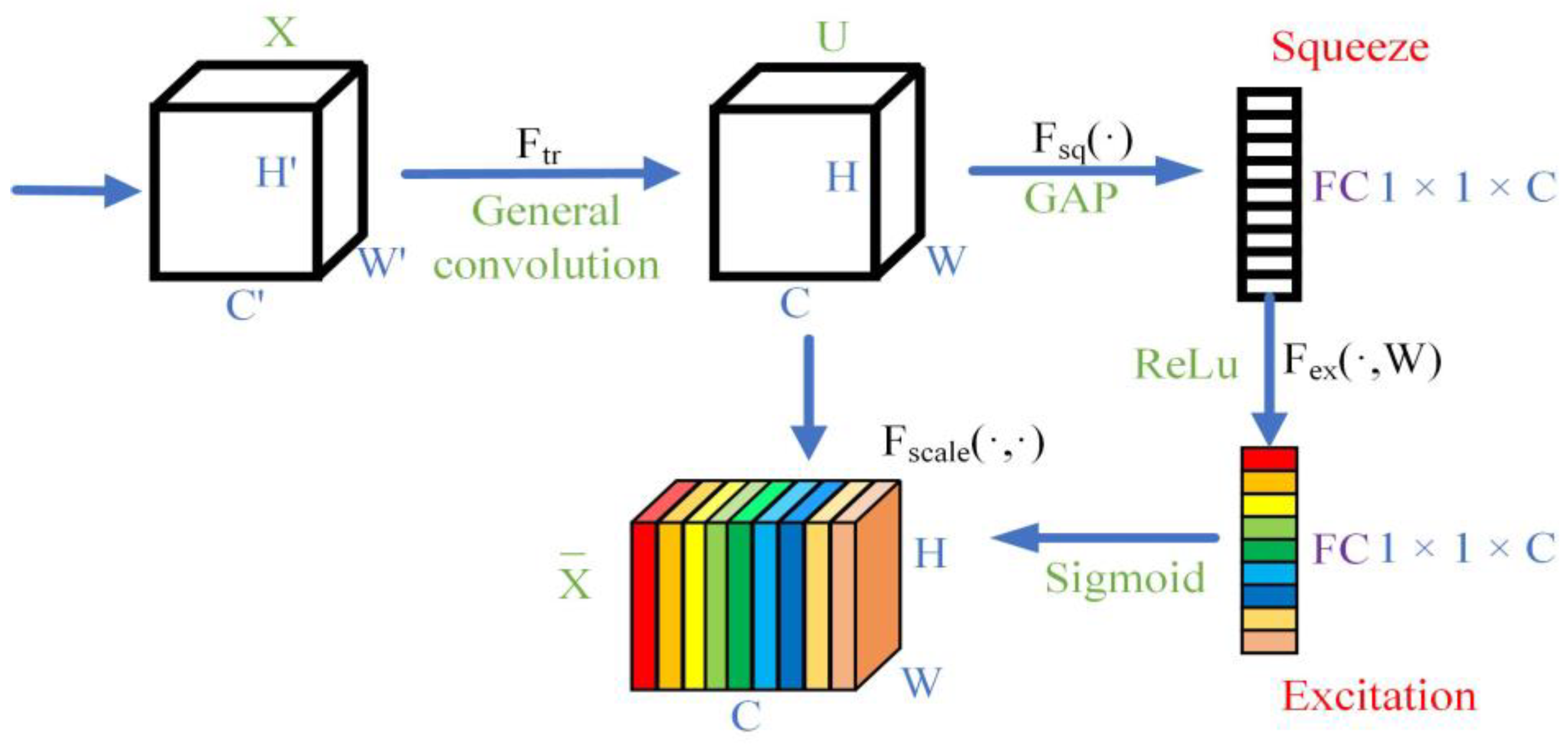
The characteristic of the SENet module is that it focuses on the relationships between channels in the hope that the model can automatically learn the importance of different channel features. After multi-layer neural network training with the data, the number of channels will naturally increase and the weight of different channels will be unequal. The SE module is an integral part of the SENet module. After using the SE module, more important weight information could be captured so that the model could obtain higher amounts of information, resulting in the accuracy naturally improving. The structure of the SE module is shown in Figure 2. It can be seen from Figure 2 that the SE module is divided into squeeze and excitation. In the squeeze part, the input feature vectors are compressed into 1 × 1 × C vectors through global averaging pooling. The primary function proposed by global averaging pooling is to replace part of the fully-connected (FC) layer, reduce the number of parameters of the fully-connected layer and regularize the whole network structure to prevent overfitting. The purpose of using global average pooling in the squeeze part is also to reduce the dimensions of the data. The compressed feature vector enters the fully-connected layer after passing the ReLu activation function. The FC layer in the first part is to reduce the amount of computation, and the data size at this part is 1 × 1 × C/r. The FC layer in the second part is to restore the data dimension to 1 × 1 × C. In the excitation part, the FC layer is restored to the original input dimension size after being stacked by the Sigmoid function and then added to the original input to get the output result.

2.3. Res2Net Module

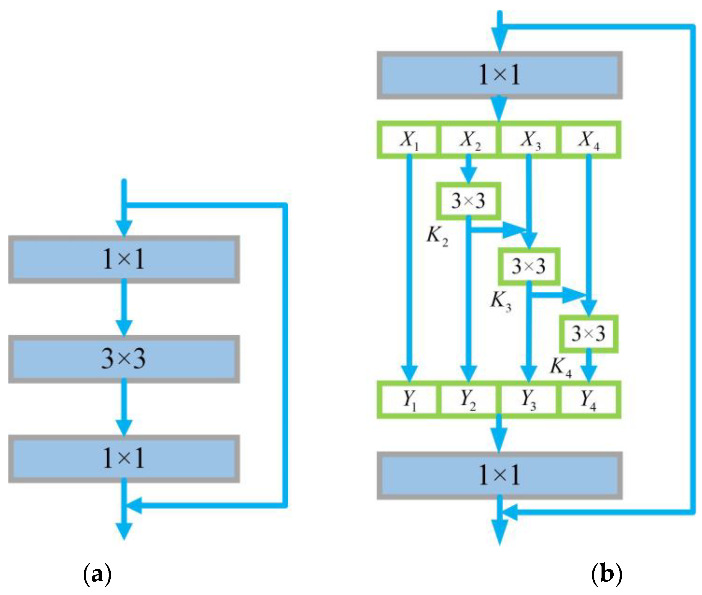
With the deepening of neural network training, more and more information can be obtained and features will be increasingly enriched. However, parameter optimization at this time is inferior and it is challenging to achieve the expected effects of the accuracy and loss functions of the training and test datasets. The common residual neural network [42] (ResNet) solved the gradient explosion and gradient disappearance caused by the deepening of the neural network to a certain extent. Res2Net is a variant of ResNet. Its main characteristic is the use of multi-scale convolution, which is widely used in the Inception [43] series of networks. Res2Net not only improves the accuracy of classification tasks but also improves the accuracy of detection tasks. It can be integrated with other excellent existing modules, and its test performance exceeds that of the ordinary residual neural network without increasing the number of calculations. The detailed structures of ResNet and Res2Net are shown in Figure 3. It can be seen from Figure 3 that Res2Net has improved ResNet by constructing a similar residual connection with hierarchy in a single residual block, replacing the general single 3 × 3 convolution kernel. Res2Net represents multi-scale features at a finer granularity level and increases the receptive field of each network layer.

2.4. SE-Res2Net Module

The SE-Res2Net model is based on the SENet and Res2Net, contains both of their advantages, and has better a training effect than either of the two modules. The specific structure before and after the combination is shown in Figure 4 (left is Res2Net module; right is SE-Res2Net module). It can be seen from Figure 4 that the SE-Res2Net module replaces the large convolution kernel by stacking small convolution kernels. Since each stacked convolutional layer contains activation functions, more nonlinear expressions can be obtained with the same receptive field and the effective performance is better.

3. Damage Diagnosis Model and Process

3.1. Structure of the Proposed Model

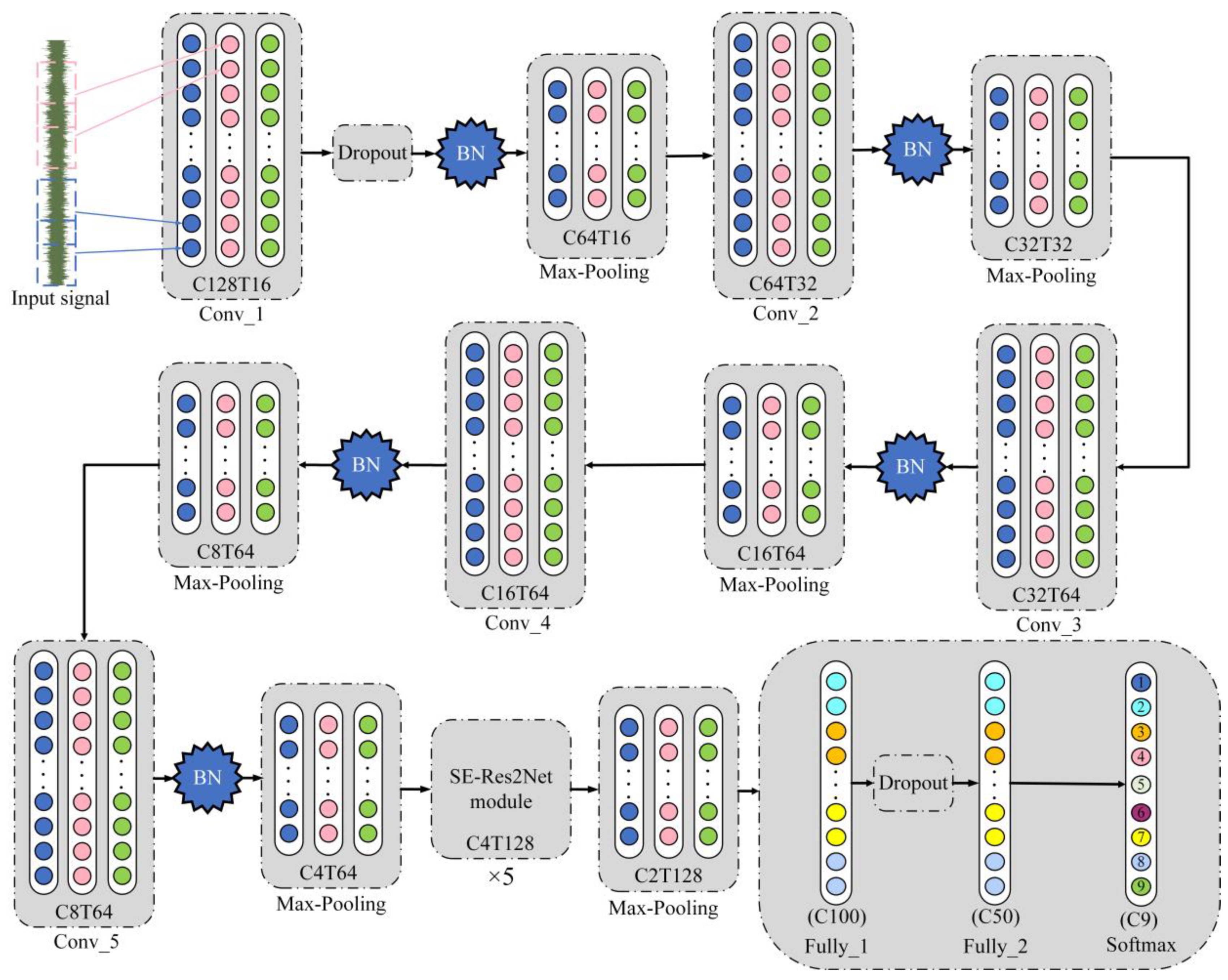
Because the accuracy of damage diagnosis of frame structures using TICNN is relatively low, this paper modified various parameters of TICNN including increased depth of the neural network and improved feature extraction ability of the model. On this basis, the SE-Res2Net module was added to form the proposed new model to obtain higher accuracy and strong anti-noise ability. The overall structure of the proposed new model is shown in Figure 5. As can be seen from Figure 5, compared with TICCN, the new model proposed in this paper reduces the step size of the first convolutional layer, increases the step size and the convolution kernel size of the second convolutional layer, reduces one set of convolution layer and pooling layer, and adds five layers of the SE-Res2Net module. In addition, a Dropout layer was added at the fully-connected layer.

3.2. Model Parameters

The parameters of the TICNN model were modified in the proposed new model. Firstly, the size of the input data was changed to 1024. Secondly, under the same experimental conditions, the influence of different step size of the first convolutional layer on the model’s accuracy was studied, and the appropriate step size was selected. The influence of the step size of the first convolutional layer on the model’s accuracy and loss functions are shown in Table 1. It shows that when the step size of the first convolutional layer is eight, the accuracy of the proposed new model is the highest, so the step size of the first convolutional layer was reduced from sixteen to eight. Thirdly, the convolution kernel size and step size of the second convolutional layer of the TICNN model were also adjusted. Then, a three-layer small convolution kernel structure and a five-layer SE-Res2Net module were added into the new model. Finally, an alternating distribution structure of three fully-connected layers and a Dropout layer were added after the SE-Res2Net modules to increase the classification accuracy of the proposed model. The convolution kernel size, step size, channels, output size and other parameters of the new model are shown in Table 2.

3.3. Damage Diagnosis Process

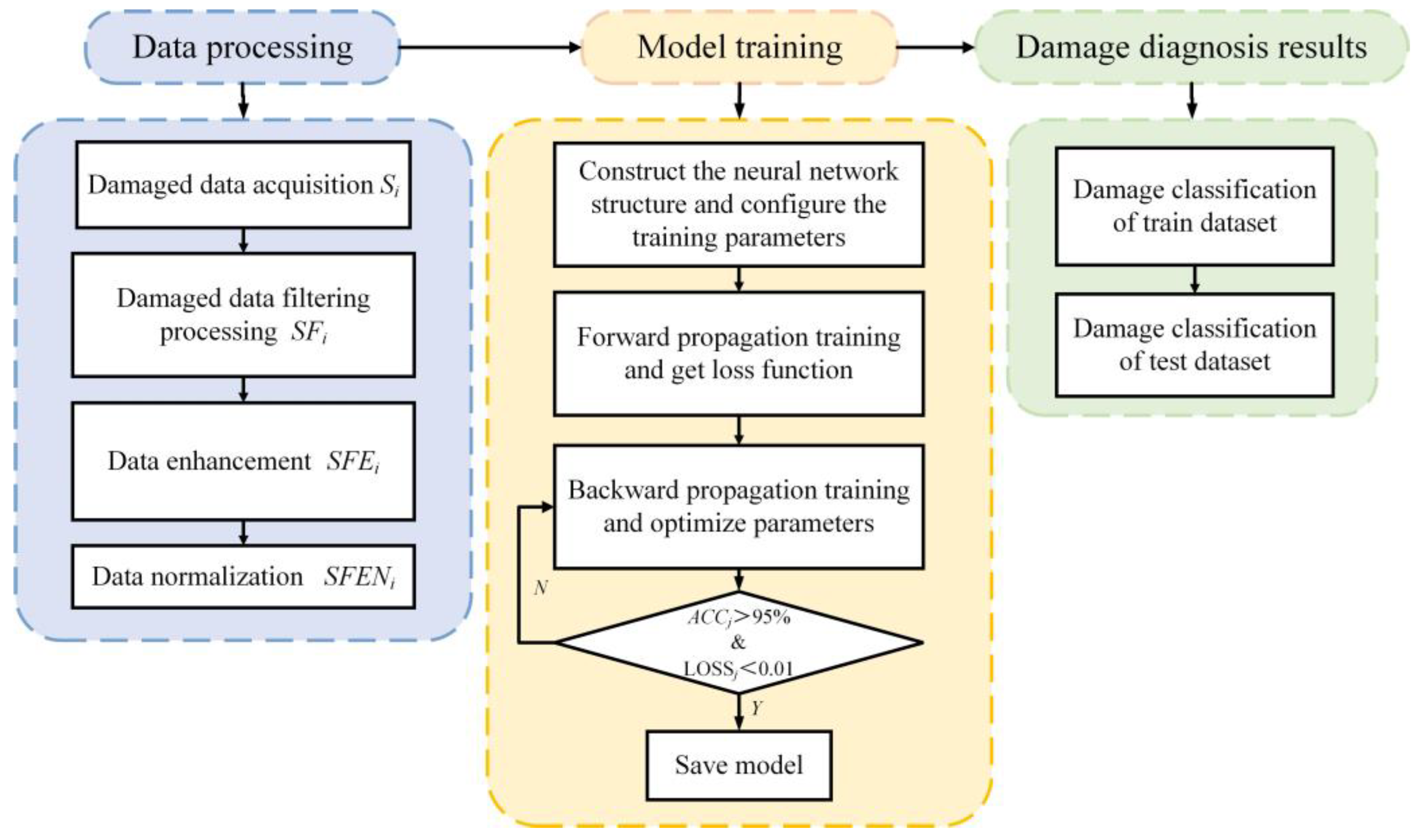
The schematic diagram of the damage diagnosis process of the frame structure is shown in Figure 6. It can be seen from Figure 6 that the whole damage diagnosis process includes data processing, model training and damage diagnosis results.
(1)
Data processing
The data processing process was as follows. Firstly, the vibration signal was collected by the sensor, then the vibration signal was filtered, and finally the vibration signal after filtering was processed by data slicing and enhancement and data normalization.
  • Data acquisition and filtering
    The data of each damage case is represented by Si, where i represents the case. Generally, the noise in the construction environment is Gaussian noise [44]. Therefore, a Gaussian low-pass filter was used to process the data collected by sensors, making it smoother, since it can reduce the influence of high-frequency noise on the results. The formula is shown in Equation (1). The filtered data is represented by SFi:
    G ( x ) = 1 σ 2 π e x 2 2 σ 2
    where σ is the standard deviation of input signal x.
  • Data slicing and enhancement
    When the number of samples in the training dataset is small, the trained model cannot complete sufficient training, which will lead to over-fitting and thus cannot meet the ideal requirements. When the number of samples in the training dataset is larger, the model can learn more features and gain stronger generalization abilities. Therefore, in order to increase the number of samples in the training dataset and improve the training results, it was necessary to adopt the sliding window method for data enhancement. Different numbers of data samples can be obtained by adjusting the size of the sliding window. The sliding window method can obtain enough data samples. The filtered data SFi after data enhancement using the sliding window method is expressed as SFEi. For example, for a signal with K vibration points, the size of sliding window is set to W, and the step of sliding window is set to S, then samples with a number of N can be obtained. The formula can be written as:
    N = K W S + 1
  • Data normalization
    Data normalization can process data according to the statistical distribution of samples. Normalized data tend to be smoother in training and can accelerate the convergence rate of the model, making the training process more stable. The dataset after data enhancement SFEi is normalized between [–1, 1], and SFENi represents the normalized data:
    S F E N i = S F E i a v e r a g e ( S F E i ) | M a x ( S F E i ) |
(2)
Model training
In model training, the structure of the model needs to be built first before the training dataset can be input into the model. The loss function of the model can be obtained after forward propagation, and the model’s parameters are optimized through backward propagation. Finally, the model which meets the training requirements is saved.
(3)
Damage diagnosis results
Damage diagnosis results can be obtained by analyzing the results of the training dataset and test dataset. The diagnostic results of the training dataset will be displayed after the training is completed. To obtain the diagnosis results of the test dataset, firstly the trained model needs to be saved and then input the test dataset into it to obtain the results. Finally, according to the classification accuracy of the training dataset and the test dataset, the performance of the model is analyzed to determine whether the damage diagnosis ability of the model meets the requirements.

4. Experiments

The contents of the experiments included: The experimental object and experimental data, damage type diagnosis experiment, comparative experiment of diagnosis accuracy and comparative experiment of anti-noise ability. The deep learning framework of these experiments was based on the TensorFlow version 2.3.1 and the configuration of the computer is as follows. CPU: Intel Core i7-10750 H, GPU: NVIDIA GTX 1660Ti.

4.1. Experimental Object

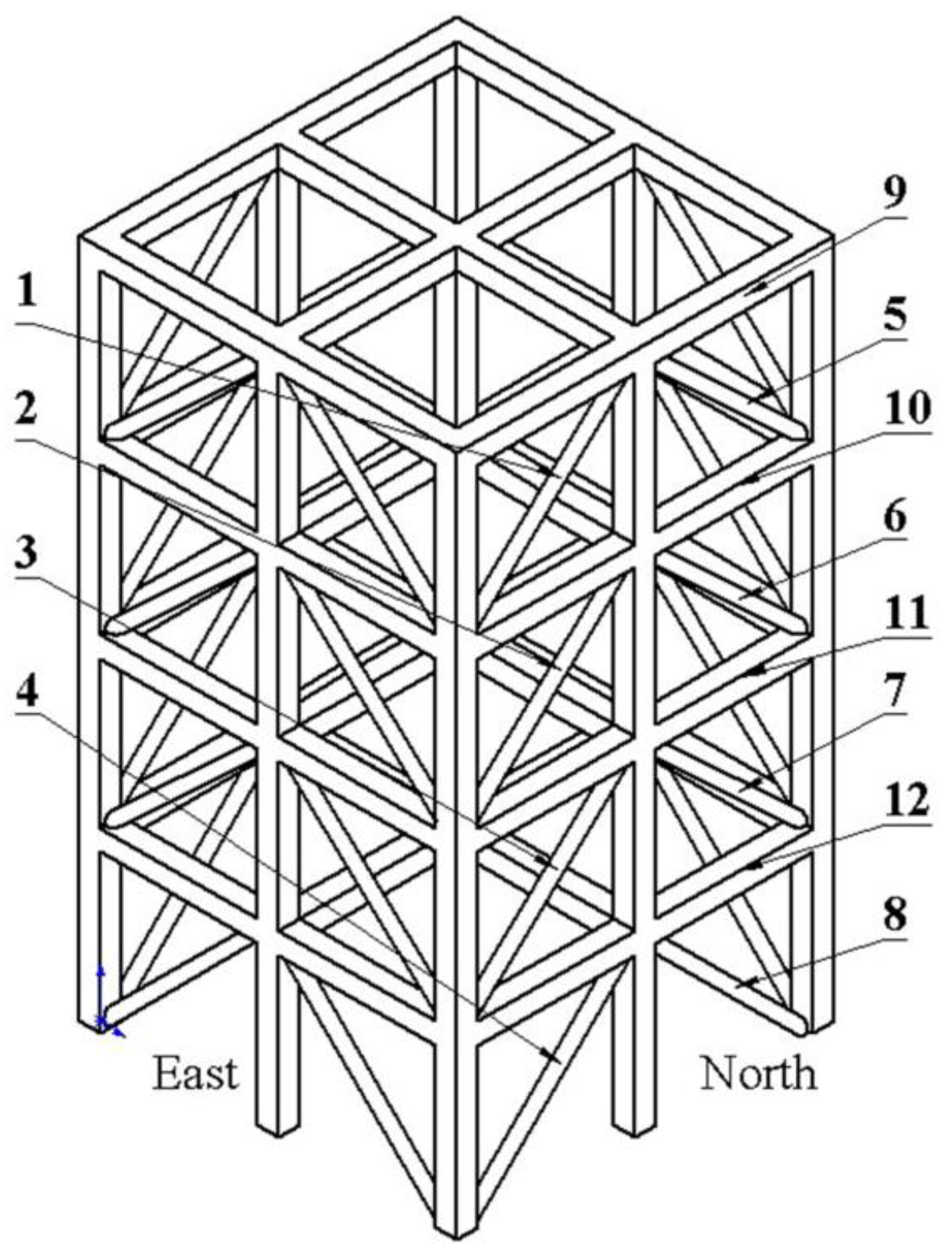
This paper took the four-layer steel frame structure model from the University of British Columbia for the research object, and its structure is shown in Figure 7. It can be seen from Figure 7 that the structure is divided into four directions: east, west, north and south, and that each direction is composed of beams and columns with the same structure. A total of 15 acceleration sensors were placed at the joints shown in the figure, with three acceleration sensors at each floor (one at the center column and one at the east and west sides). Acceleration sensors numbered 1, 2 and 3 were placed at the lowest floor close to the ground, and the rest were placed at the top of each floor.
By removing or loosening the structure at the locations numbered 1–12 in the figure, a total of nine different damage cases were obtained. The details of each case are shown in Table 3. As seen from Figure 7 and Table 3, the overall degree of damage of the frame structure in nine cases was different, meaning that the collected vibration data were quite different. Therefore, nine damage cases can be distinguished according to the vibration data.

4.2. Experimental Data

The acquisition of vibration data is generally collected through environmental excitation, hammer tapping, random excitation (5–50 Hz) and other methods. In this experiment, the vibration data were obtained by applying 200 Hz excitation to the frame structure.
Since the vibration exciter was installed at the top, the sensor at the bottom was the most stable when damage occurred. Since the sensors numbered 1, 2 and 3 were close to the ground, to avoid errors in the results, the vibration data collected by the sensor numbered 5 at the center column of the second layer were selected for damage diagnosis of the frame structure.
According to the official dataset of the University of British Columbia, the signal length of cases 1–5 is 24,000, and cases 6–9 is 60,000, 72,000, 72,000, 72,000, respectively. In order to make the number of samples in the training and test datasets consistent, the size of the sliding window selected was 1024, the step of the sliding window of cases 1–5 were 24, case 6 was 60 and cases 7–9 were 72.

4.3. Damage Type Diagnosis Experiment

(1)
Analysis of training results
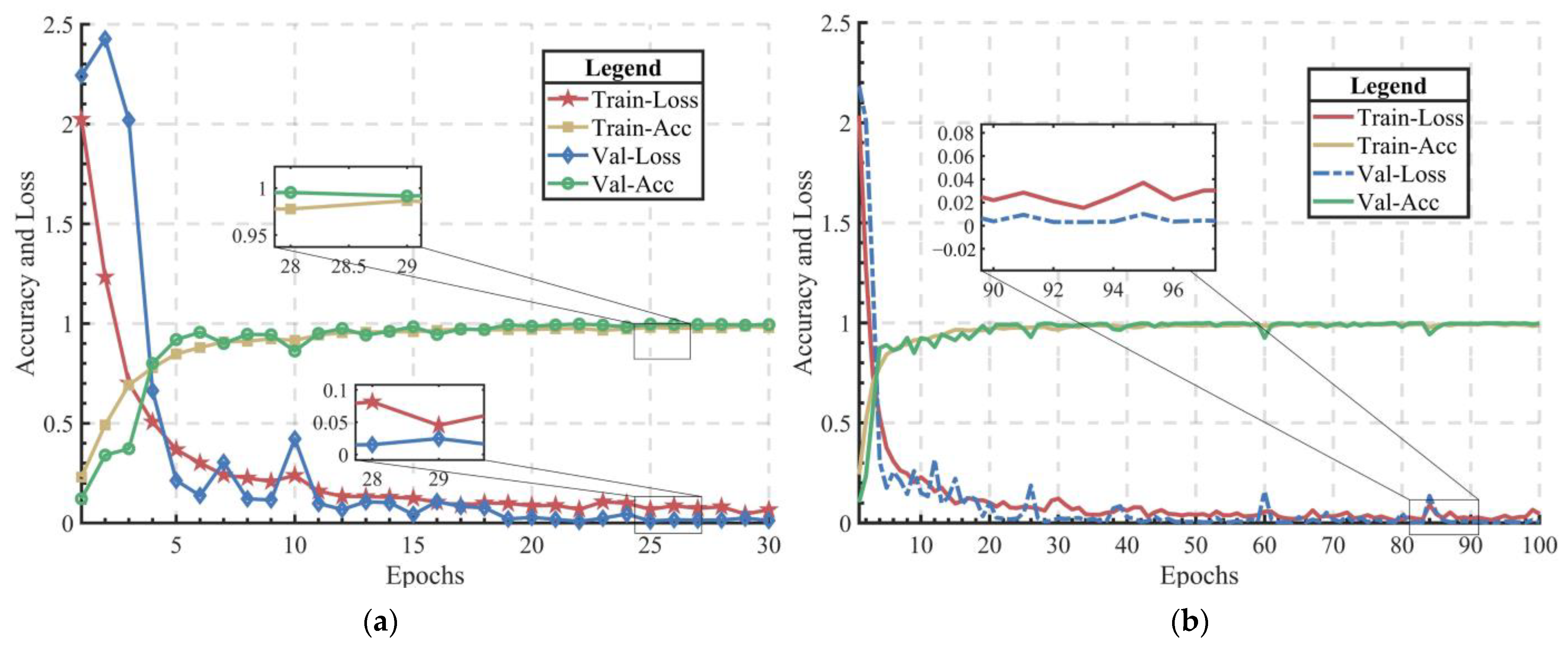
In the process of model training, Adam was used as the optimizer and the initial learning rate was set to 0.001. The training curves of the nine damage cases of the frame structure are shown in Figure 8. In order to show the training results more clearly, the curves of training epoch = 30 and training epoch = 100 were drawn, respectively. It can be seen from the figures that when the training epoch reaches 4, the training results begin to converge, the accuracy gradually rises to more than 90% and the loss begins to be less than 0.1. When the training epoch reaches 30, the loss of the training and the validation dataset reach about 0.02, and the accuracy is also higher than 98%. When the training epoch reaches 100, the loss curves tend to be gentle and fluctuate at epochs = 25, 60 and 85, respectively. The final loss is about 0.009, which shows that the proposed new model can achieve higher classification accuracy.
(2)
Confusion matrix analysis
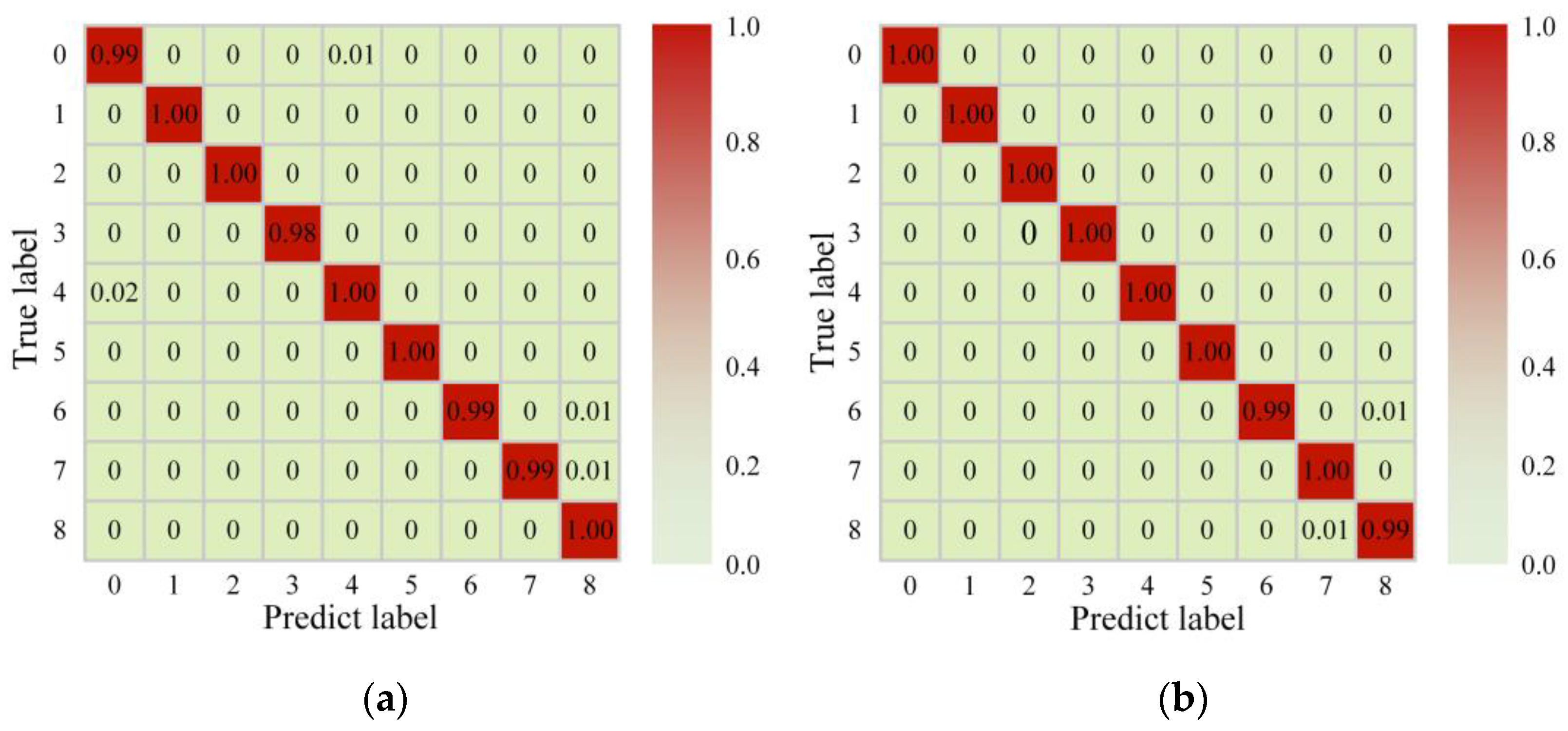
The confusion matrix can count the number of true and predict labels in the model diagnosis results, which is a method to evaluate the model’s performance. By calculating the ratio between the number of true and predict labels in the confusion matrix, a series of classification indicators such as accuracy, precision, recall and sensitivity can be obtained to judge the diagnosis effect of the neural network model. The confusion matrix training results are shown in Figure 9. In order to correspond to the training curves and express the training results more clearly, the confusion matrices of training epoch = 30 and training epoch = 100 were drawn, respectively.
It can be seen from Figure 9 that the accuracy is 99.44% when the training epoch reaches 30 and 99.78% when training epoch reaches 100. From the figures, it can be clearly distinguished which kinds of damage classification of the model have deviation, which is also the aspect that needs to be focused on in later research.
(3)
T-SNE visualization
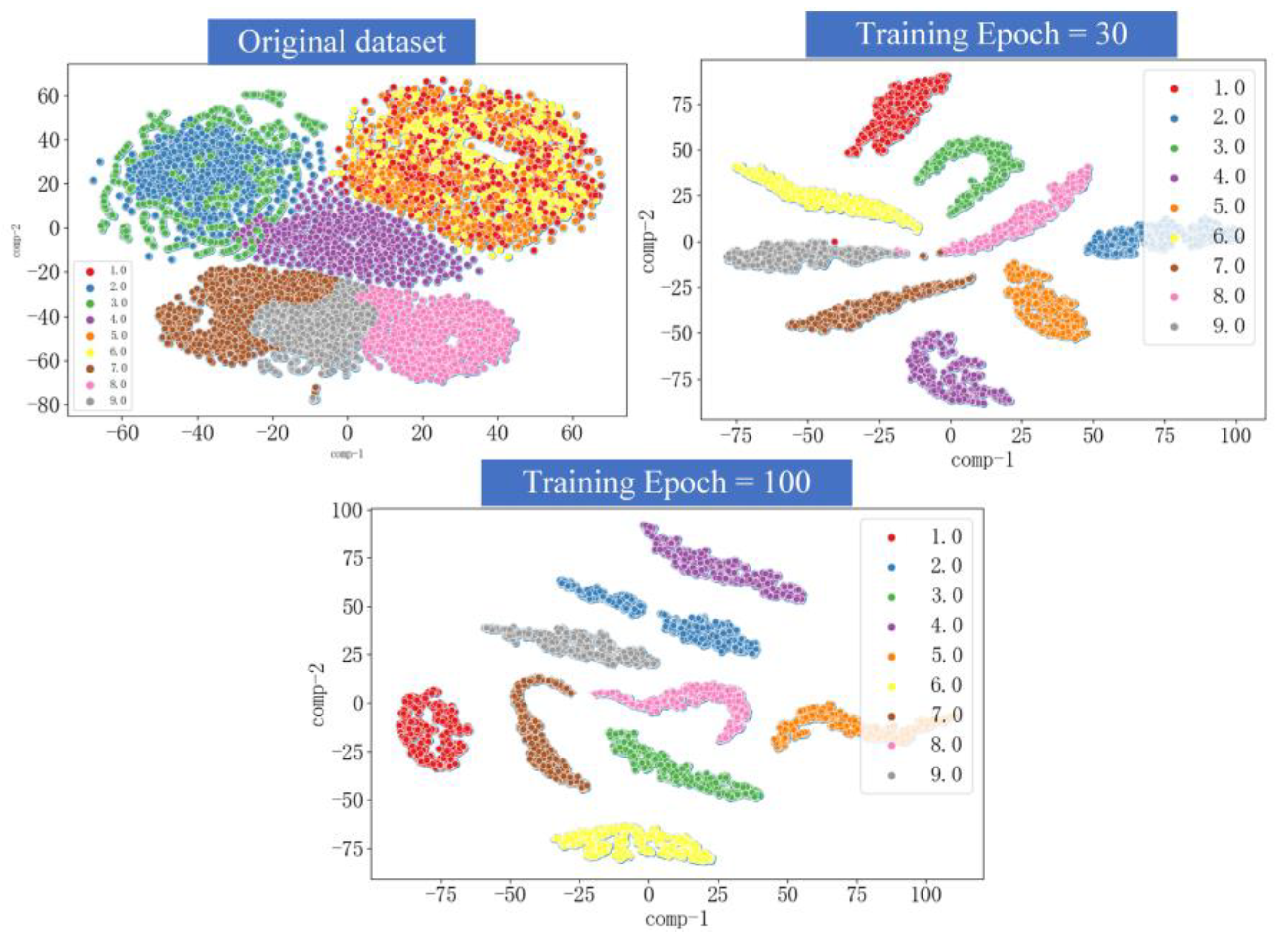
T-Distributed Stochastic Neighbor Embedding (T-SNE) is a dimensionality reduction technique for visualizing high-dimensional data. The T-SNE has a non-convex objective function, which is optimized by a randomly initialized gradient descent method so that different results may be obtained each time.
In this section, the original data, the result of training epoch = 30 and the result of training epoch = 100 were visually analyzed. The results are shown in Figure 10. From the figure, it can be seen that the original dataset of nine damage cases is very confusing. After 30 epochs training, in addition to sporadic dispersion at the edge of damage case 8 and case 9, the other damage cases can be clearly distinguished. After 100 epochs training, nine damage cases can be completely and clearly distinguished, and the effect is ideal.
(4)
Analysis of test dataset results
The test process needs to save the trained model first, and then input the test dataset into the saved model to obtain the diagnosis results. The confusion matrix displays the diagnosis results of the test dataset, as seen in Figure 11. It can be seen from the data in Figure 11 that the data in other positions are zero—except the data on the diagonal line is 1.0—so it is easy to calculate the accuracy and recall based on the data in the figure. According to the data calculations of the confusion matrix in Figure 11, the accuracy of the test dataset reached 100% and the recall was also 100%. This shows that the proposed new model has an ideal requirement for the classification ability of damage types.

4.4. Comparative Experiment of Diagnostic Accuracy

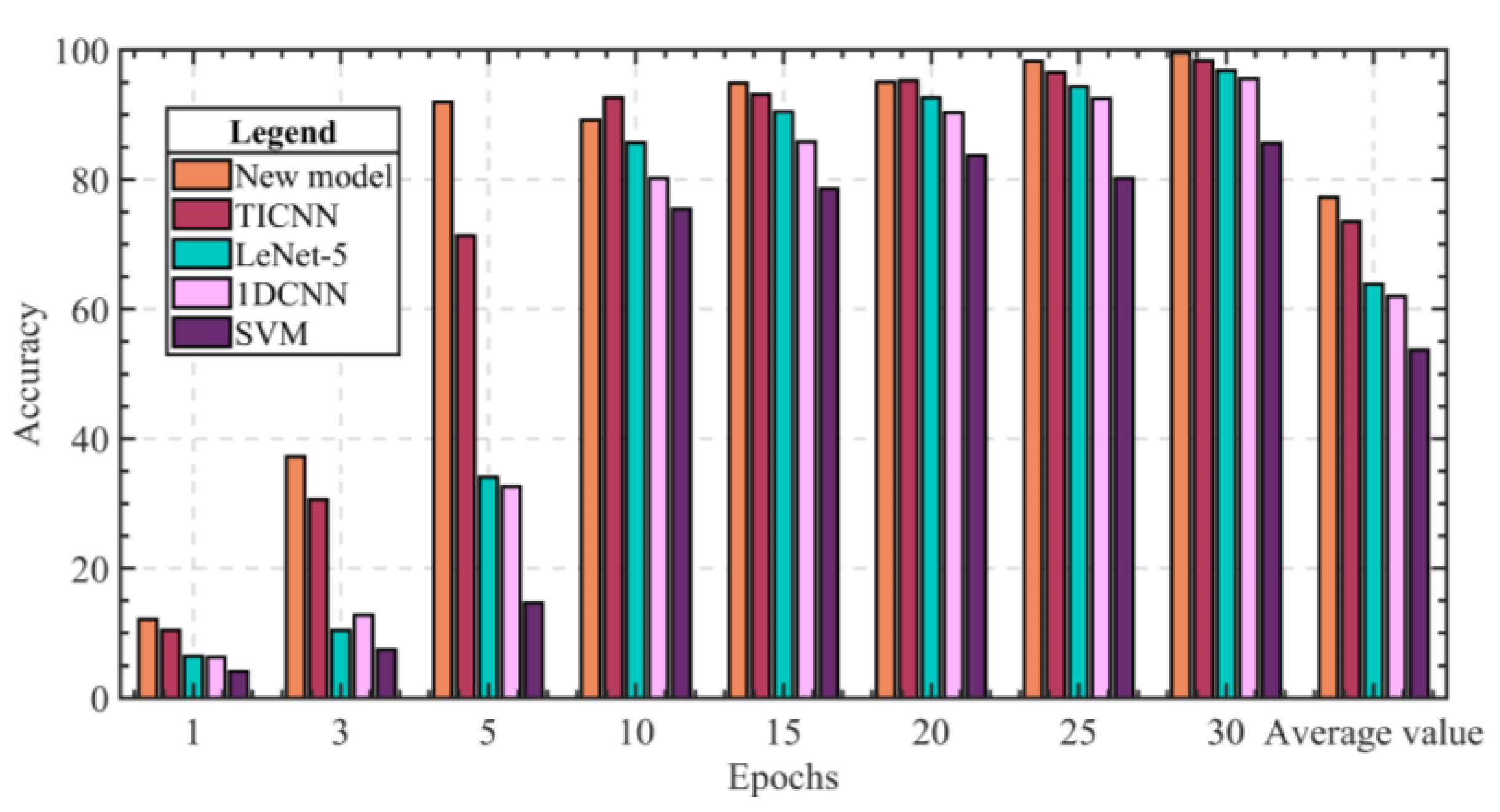
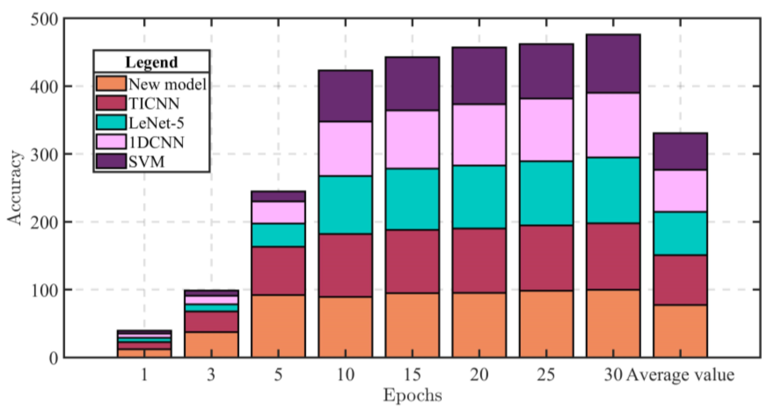
In order to verify the superiority of the proposed model for damage diagnosis, the accuracy comparison experiments were carried out with TICNN, two-dimensional model LeNet-5, 1DCNN and support vector machine (SVM). The convolution kernel, pooling layer, fully-connected layer and activation function between each layer of LeNet-5 were not changed. The structure and parameters of 1DCNN were the same as those used by Avci in reference [37], and the Gaussian kernel function was adopted in the SVM model. The accuracy and its average value of the above five models when the training epoch is equal to 1, 3, 5, 10, 15, 20, 25 and 30 are shown in Table 4, and the data in Table 4 are plotted in Figure 12 and Figure 13.
As can be seen from the data in Table 4, when the training epoch is equal to 1, the accuracy of the new model is 12.1%, the accuracy of TICNN is 10.5% and the accuracy of the other three models is all lower than 10%. When the training epoch is equal to 5, the accuracy of the new model is 91.9%, the accuracy of TICNN is 71.4% and the accuracy of the other three models is all lower than 35%. When the training epoch reaches 30, the accuracy of the new model is 99.6%, the accuracy of TICNN is 98.4%, the accuracy of LeNet-5 is 96.8%, the accuracy of 1DCNN is 95.5% and the accuracy of SVM is 85.6%. From all of the eight sets of data, although the accuracy of the new model is slightly lower than that of TICNN for two sets, on the whole, the accuracy of the new model is significantly higher than that of TICNN and the convergence speed is faster. In addition, from the average values of accuracy, the accuracy of the new model is 77.3%, which is 3.8% higher than that of TICNN, and the accuracy of other models is below 65%. It can also be seen from Figure 12 and Figure 13 that the diagnostic capability of the new model is superior to other models.

4.5. Comparative Experiment of Anti-Noise Ability

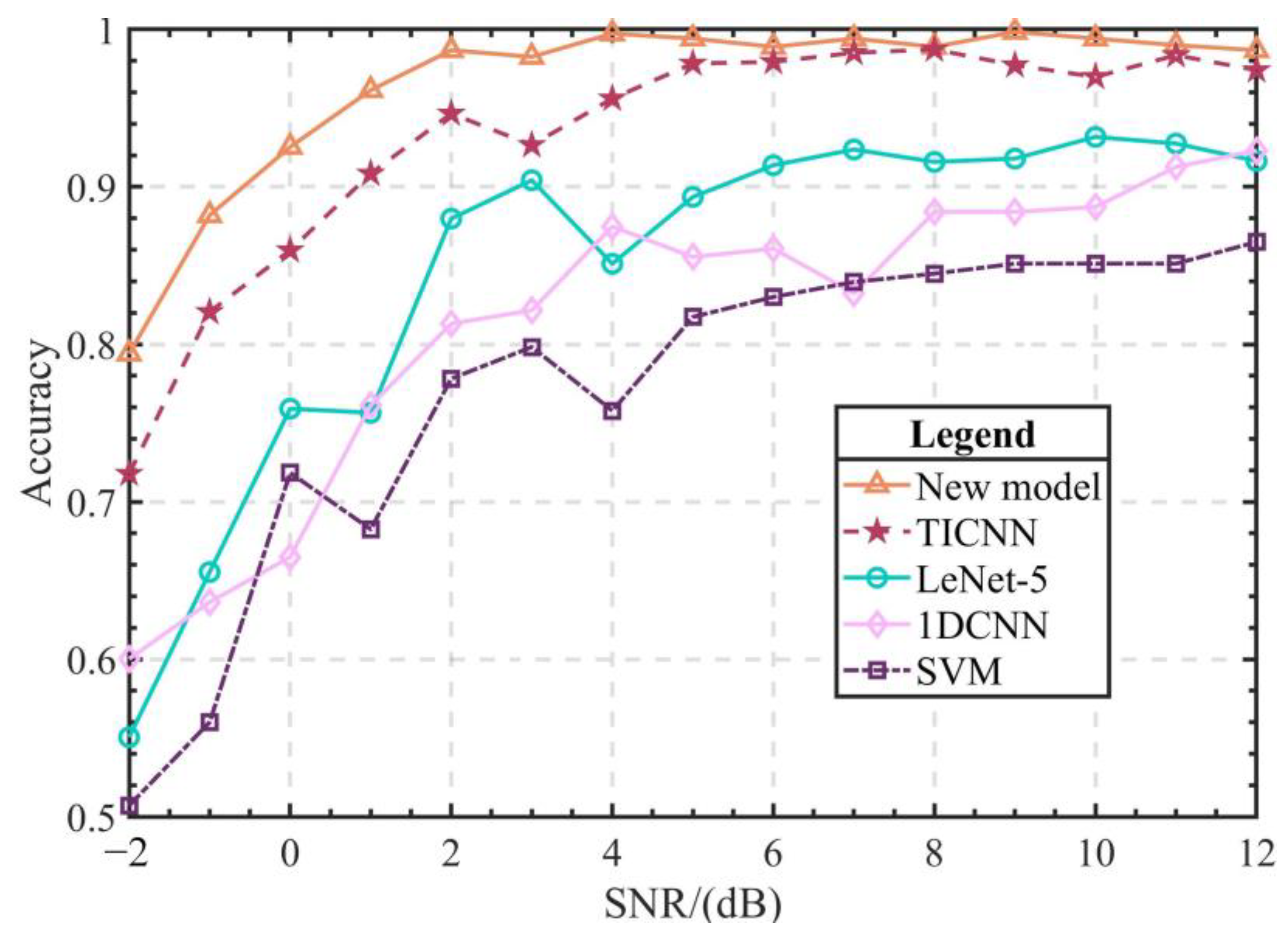
The comparative experiment of anti-noise ability also used the above models. Firstly, the Gaussian white noise with different signal-to-noise ratio (SNR: −2~12 dB) was added to the original signal. Then the data after added noise were used as the input of the above models to obtain the diagnosis results. Finally, the accuracy of the five models was compared. The results are shown in Figure 14. The figure shows that the new model has excellent advantages in accuracy and stability compared with the shallow SVM model and LeNet-5 model. The new model performs well under different SNRs. The accuracy of the new model is about 80% when the SNR is −2 dB, while that of TICNN is 72% and that of 1DCNN is 60%. The diagnostic results of both are lower than that of the new model, so it can be concluded that the new model proposed in this paper is more reliable under the condition of strong noise for damage diagnosis of frame structures.

5. Conclusions

In order to improve the damage diagnosis accuracy of frame structures in strong noise environments, a new neural network model was proposed based on the convolution neural network with training interference which has excellent performance in bearing fault recognition. Meanwhile, the proposed new model used a squeeze-and-excitation neural network and Res2Net module which are excellent in image recognition. Taking the frame structure model from the University of British Columbia as the experimental object, the proposed new model was used in a damage type diagnosis experiment. In order to verify the superiority of the proposed new model, convolution neural network with training interference, LeNet-5, one-dimensional convolutional neural network and support vector machine were used under the same conditions to compare their accuracy and anti-noise ability. The following conclusions can be drawn from the experimental study.
(1)
The training process of the proposed new model has a fast convergence speed and high multi-classification accuracy; the accuracy of the training dataset is 99.78% and the accuracy of the test dataset is 100%.
(2)
Compared with other similar models, the proposed new model has the highest accuracy of 99.6% when the training epoch reaches 30, and the average value of accuracy can reach 77.3%, which is higher than other models. Therefore, the proposed new model can achieve higher accuracy in the early stage of training and has better performance than other models.
(3)
In the comparative experiment of anti-noise ability, the anti-noise ability of the proposed new model is about 4~5% stronger than that of convolution neural network with training interference. Compared with other models, the new model performs better and has stronger anti-noise performance. It can accurately diagnose the damage of a structural frame in a strong noise environment.

Author Contributions

W.F., formal analysis, software, investigation, validation and writing—original draft; Z.L., methodology, formal analysis, software, supervision and writing—original draft; C.C., funding acquisition, methodology, project administration, formal analysis and writing—review and editing; Y.X., methodology, formal analysis, investigation and writing—review and editing; J.R., formal analysis, investigation and writing—review and editing. All authors have read and agreed to the published version of the manuscript.

Funding

This work was supported by the Nature Science Foundation of Hebei Province, grant no. E2020402060; Key Laboratory of Intelligent Industrial Equipment Technology of Hebei Province (Hebei University of Engineering), grant no. 202206; and Key Research and Development Project in Hebei Province, grant no. 19211906D.

Institutional Review Board Statement

Not applicable.

Informed Consent Statement

Not applicable.

Data Availability Statement

Data sharing not applicable.

Conflicts of Interest

The authors declare no conflict of interest.

References

  1. Zeng, Z. Application and Development of Neural Network Technology in Mechanical Engineering. Sci. Technol. Innov. Appl. 2020, 18, 153–154. [Google Scholar]
  2. Gul, M.; Catabas, N. Structural health monitoring and damage assessment using a novel time series analysis methodology with sensor clustering. J. Sound Vib. 2011, 330, 1196–1210. [Google Scholar] [CrossRef]
  3. Yin, X. Discussion on the existing problems and Solutions in contemporary civil construction. Sci. Technol. Innov. Appl. 2013, 32, 241–248. [Google Scholar]
  4. Shun, L.; Hai, G.; Dian, L. Review of Vibration signal Processing Methods. Chin. J. Sci. Instrum. 2013, 34, 1907–1915. [Google Scholar]
  5. Heng, L.; Hydrogen, Z.; Xian, Q. Bearing Fault Diagnosis Method Based on Short-time Fourier Transform and Convolutional Neural Network. J. Vib. Shock 2018, 37, 124–131. [Google Scholar]
  6. Zhi, L.; Ming, Z.; Fu, C. Research on Mechanical Fault Diagnosis Method Based on Empirical Wavelet Transform. Chin. J. Sci. Instrum. 2014, 35, 2423–2432. [Google Scholar]
  7. Huang, P.; Liao, G.; Yang, Z. A fast SAR imaging method for ground moving target using a second-order WVD transform. IEEE Trans. Geosci. Remote Sens. 2015, 54, 1940–1956. [Google Scholar] [CrossRef]
  8. Manhertz, G.; Bereczky, A. STFT spectrogram based on hybrid evaluation method for rotating machine transient vibration analysis. Mech. Syst. Signal Process. 2021, 154, 107583. [Google Scholar] [CrossRef]
  9. Deng, W.; Zhang, S.; Zhao, H. A novel fault diagnosis method based on integrating empirical wavelet transform and fuzzy entropy for motor bearing. IEEE Access 2018, 6, 35042–35056. [Google Scholar] [CrossRef]
  10. Singru, P.; Krishnakumar, V.; Natarajan, D. Bearing failure prediction using Wigner-Ville distribution, modified Poincare mapping and fast Fourier transform. J. Vibro Eng. 2018, 20, 127–137. [Google Scholar] [CrossRef] [Green Version]
  11. Zhang, C.; Yuan, G.; Ming, M. Review on the development and application of Artificial Neural network model. Comput. Eng. Appl. 2021, 57, 57–69. [Google Scholar]
  12. Zhang, S.; Li, X.; Zong, M. Efficient KNN classification with different numbers of nearest neighbors. IEEE Trans. Neural Netw. Learn. Syst. 2017, 29, 1774–1785. [Google Scholar] [CrossRef]
  13. Gen, Y.; Wang, J.; Jin, L. Application of Decision Tree Algorithm in Diagnosis Machinery Fault Information Mining. Mach. Des. Manuf. 2022, 371, 168–176. [Google Scholar]
  14. Chen, M.; Ming, L.; Qiang, G. Rolling Bearing Fault Diagnosis Based on Sparrow Search Algorithm Optimization Support Vector Machine. Sci. Technol. Eng. 2021, 21, 4025–4029. [Google Scholar]
  15. Saravanan, N.; Ramachandran, K.I. Incipient gear box fault diagnosis using discrete wavelet transform (DWT) for feature extraction and classification using artificial neural network (ANN). Expert Syst. Appl. 2010, 37, 4168–4181. [Google Scholar] [CrossRef]
  16. Lu, J.; Qian, W.; Li, S. Enhanced K-nearest neighbor for intelligent fault diagnosis of rotating machinery. Appl. Sci. 2021, 11, 919. [Google Scholar] [CrossRef]
  17. Yan, X.; Jia, M. A novel optimized SVM classification algorithm with multi-domain feature and its application to fault diagnosis of rolling bearing. Neurocomputing 2018, 313, 47–64. [Google Scholar] [CrossRef]
  18. Jie, G.; Xian, X. Research on transformer fault diagnosis based on support vector machine. Hydropower N. Energy 2020, 34, 28–31. [Google Scholar]
  19. Zoph, B.; Vasudevan, V.; Shlens, J. Learning transferable architectures for scalable image recognition. In Proceedings of the IEEE Conference on Computer Vision and Pattern Recognition (CVPR), Salt Lake City, UT, USA, 18–23 June 2018; IEEE: Piscataway, NJ, USA, 2018; pp. 8697–8710. [Google Scholar]
  20. Henaff, O. Data-efficient image recognition with contrastive predictive coding. In Proceedings of the 37th International Conference on Machine Learning, Virtual, 13–18 July 2020; Volume 39, pp. 4182–4192. [Google Scholar]
  21. Sharma, N.; Jain, V.; Mishra, A. An analysis of convolutional neural networks for image classification. Procedia Comput. Sci. 2018, 132, 377–384. [Google Scholar] [CrossRef]
  22. Lguensat, R.; Tandeo, P.; Ailliot, P. The analog data assimilation. Mon. Weather Rev. 2017, 145, 4093–4107. [Google Scholar] [CrossRef] [Green Version]
  23. Lv, L.; Li, D.; Cui, C. Nuclease-aided target recycling signal amplification strategy for ochratoxin A monitoring. Biosens. Bioelectron. 2017, 87, 136–141. [Google Scholar] [CrossRef]
  24. Zhao, Y.; Shi, Y.; Wang, Z. The Improved YOLOV5 Algorithm and Its Application in Small Target Detection. In Proceedings of the Intelligent Robotics and Applications: 15th International Conference, ICIRA 2022, Harbin, China, 1–3 August 2022; Springer International Publishing: Cham, Switzerland, 2022; pp. 679–688. [Google Scholar]
  25. Wang, Y.; Yan, J.; Yang, Z. A novel 1DCNN and domain adversarial transfer strategy for small sample GIS partial discharge pattern recognition. Meas. Sci. Technol. 2021, 32, 122–131. [Google Scholar] [CrossRef]
  26. Simonyan, K.; Zisserman, A. Very Deep Convolutional Networks for Large-Scale Image Recognition; ICLR.UK: University of Oxford: Oxford, UK, 2015; pp. 1–7. [Google Scholar]
  27. Krizhevsky, A.; Sutskever, I.; Hinton G, E. Imagenet classification with deep convolutional neural networks. Commun. ACM 2017, 60, 84–90. [Google Scholar] [CrossRef] [Green Version]
  28. Zeiler M, D.; Fergus, R. Visualizing and understanding convolutional networks. In Proceedings of the Computer Vision–ECCV 2014: 13th European Conference, Zurich, Switzerland, 6–12 September 2014; Springer International Publishing: Berlin/Heidelberg, Germany, 2014; pp. 818–833. [Google Scholar]
  29. Zhang, Y.; Wang, J.; Zhang, X. Conciseness is better: Recurrent attention LSTM model for document-level sentiment analysis. Neurocomputing 2021, 462, 144–156. [Google Scholar] [CrossRef]
  30. Jiang, H.; Qin, F.; Cao, J. Recurrent neural network from adder’s perspective: Carry-lookahead RNN. Neural Netw. 2021, 144, 13–21. [Google Scholar] [CrossRef]
  31. Wang, D.; Tang, L.; Zhu, J. Dairy goat detection based on Faster R-CNN from surveillance video. Comput. Electron. Agric. 2018, 154, 55–63. [Google Scholar] [CrossRef]
  32. Zheng, J.; Min, C.; Jun, C. Multi-scale Fuzzy Entropy and Its Application in Rolling Bearing Fault Diagnosis. J. Vib. Eng. 2014, 27, 145–151. [Google Scholar]
  33. Tamilselvan, P.; Wang, P. Failure diagnosis using deep belief learning based health state classification. Reliab. Eng. Syst. Saf. 2013, 115, 124–135. [Google Scholar] [CrossRef]
  34. Song, H.; Hai, S. Intelligent Fault Diagnosis of aero-engine High-speed Bearing Based on Elevated Convolutional Neural Network. J. Aeronaut. Astronaut. 2021, 43, 1–15. [Google Scholar]
  35. Janssens, O.; Slavkovikj, V.; Vervisch, B. Convolutional neural network based on fault detection for rotating machinery. J. Sound Vib. 2016, 377, 331–345. [Google Scholar] [CrossRef]
  36. Wang, J.; Zhuang, J.; Duan, L. A multi-scale convolution neural network for featureless fault diagnosis. In Proceedings of the 2016 International Symposium on Flexible Automation (ISFA), Cleveland, OH, USA, 1–3 August 2016; IEEE: Piscataway, NJ, USA, 2016; pp. 65–70. [Google Scholar]
  37. Abdeljaber, A.; Younis, O.; Avci, N.; Kiranyaz, S. 1-DCNNs for structural damage detection: Verification on a structural health monitoring benchmark data. Neurocomputing 2018, 275, 1308–1317. [Google Scholar] [CrossRef]
  38. Dyke S, J.; Bernal, D.; Beck, J. Experimental phase II of the structural health monitoring benchmark problem. In Proceedings of the 16th ASCE Engineering Mechanics Conference, Chicago, IL, USA, 17 July 2003; ASCE: Reston, VA, USA, 2003; pp. 1–9. [Google Scholar]
  39. Zhang, W.; Chuan, L.; Peng, G. A deep convolutional neural network with new training methods for bearing fault diagnosis under noisy environment and different working load. Mech. Syst. Signal. Process. 2018, 100, 349–543. [Google Scholar] [CrossRef]
  40. Hu, J.; Shen, L.; Sun, G. Squeeze-and-excitation networks. In Proceedings of the IEEE Conference on Computer Vision and Pattern Recognition, Salt Lake City, UT, USA, 18–23 June 2018; IEEE: Piscataway, NJ, USA, 2018; pp. 7132–7141. [Google Scholar]
  41. Gao, S.; Cheng, M.; Zhao, K. Res2net: A new multi-scale backbone architecture. IEEE Trans. Pattern Anal. Mach. Intell. 2019, 43, 652–662. [Google Scholar] [CrossRef] [Green Version]
  42. He, K.; Zhang, X.; Ren, S.; Sun, J. Deep residual learning for image recognition. In Proceedings of the IEEE Conference on Computer Vision and Pattern Recognition, Las Vegas, NV, USA, 27–30 June 2016; IEEE: Piscataway, NJ, USA, 2016; pp. 770–778. [Google Scholar]
  43. Szegedy, C.; Ioffe, S.; Vanhoucke, V.; Alemi, A. Inception-v4, inception-resnet and the impact of residual connections on learning. In Proceedings of the AAAI Conference on Artificial Intelligence, San Francisco, CA, USA, 4–9 February 2017; AAAI: Washington, DC, USA, 2017; pp. 1–15. [Google Scholar]
  44. Xiao, W.; Jiu, S. A novel Gaussian noise filtering Algorithm. J. Beihua Univ. 2011, 12, 606–609. [Google Scholar]
  45. Ren, J.; Cai, C.; Chi, Y.; Xue, Y. Integrated Damage Location Diagnosis of Frame Structure Based on Convolutional Neural Network with Inception Module. Sensors 2022, 23, 418. [Google Scholar] [CrossRef]
  46. Xu, H.; Cai, C.; Chi, Y. Damage Location Diagnosis of Frame Structure Based on a Novel Convolutional Neural Network. Appl. Sci. 2022, 12, 12411. [Google Scholar] [CrossRef]
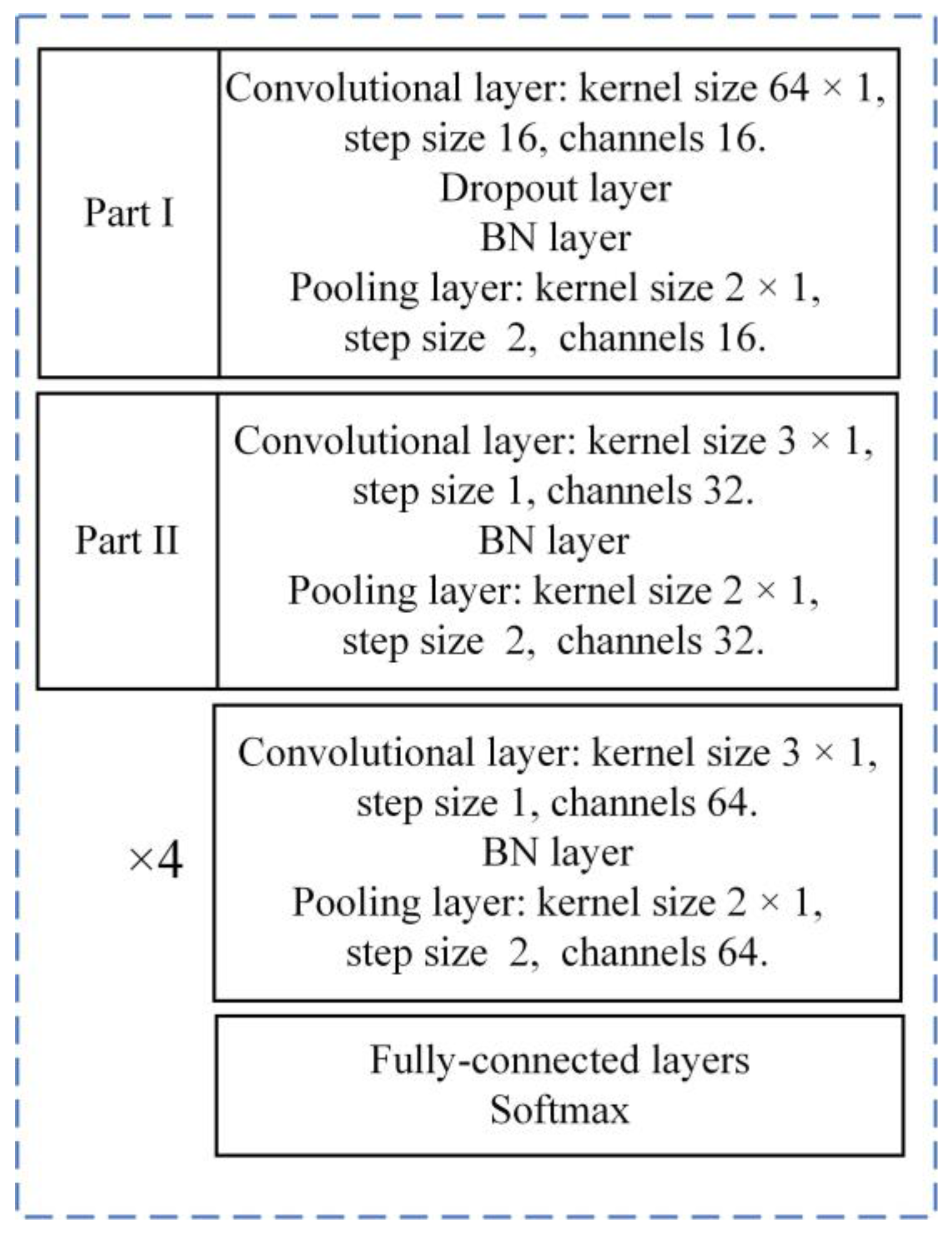
Figure 1. Structure and parameters of TICNN model.
Applsci 13 02545 g001
Figure 2. Structure of SE module [40] (The colors represent channels with different weights).
Applsci 13 02545 g002
Figure 3. Structure of ResNet and Res2Net [41]. (a) ResNet. (b) Res2Net.
Applsci 13 02545 g003
Figure 4. Structure of Res2Net and SE-Res2Net. (a) Res2Net. (b) SE-Res2Net.
Applsci 13 02545 g004
Figure 5. Structure of the proposed new model (The colors represent different feature values).
Applsci 13 02545 g005
Figure 6. The schematic diagram of damage diagnosis process.
Applsci 13 02545 g006
Figure 7. Three-dimensional model of the four-layer steel frame structure [45,46]. (The blue arrows are the coordinate systems created in drawing the 3D model).
Applsci 13 02545 g007
Figure 8. Training results. (a) Training epoch = 30. (b) Training epoch = 100.
Applsci 13 02545 g008
Figure 9. Confusion matrices of training dataset. (a) Training epoch = 30. (b) Training epoch = 100.
Applsci 13 02545 g009
Figure 10. Results of T-SNE visualization.
Applsci 13 02545 g010
Figure 11. Confusion matrix of test dataset.
Applsci 13 02545 g011
Figure 12. Experimental results of accuracy comparison (Bar chart).
Applsci 13 02545 g012
Figure 13. Experimental results of accuracy comparison (Stack bar chart).
Applsci 13 02545 g013
Figure 14. Comparison results of anti-noise capability.
Applsci 13 02545 g014
Table 1. Selection basis of the step size of the first convolutional layer.
Step Size481216202432
Accuracy0.98230.99760.99140.98620.99070.98420.9855
Loss0.00820.00340.01100.00930.01060.01630.0156
Table 2. Structure and parameters of the new model.
Layer TypeKernel/Step SizeChannelsOutput Size
(Width × Depth)
Zero Padding
Conv_164 × 1/8 × 116128 × 16Yes
Max-pooling2 × 1/2 × 11664 × 16No
Conv_232 × 1/4 × 13264 × 32Yes
Max-pooling2 × 1/2 × 13232 × 32No
Conv_33 × 1/1 × 16432 × 64Yes
Max-pooling2 × 1/2 × 16416 × 64No
Conv_43 × 1/1 × 16416 × 64Yes
Max-pooling2 × 1/2 × 1648 × 64No
Conv_53 × 1/1 × 1648 × 64Yes
Max-pooling2 × 1/2 × 1644 × 64No
SE-Res2Net_1 1284 × 128
SE-Res2Net_2 1284 × 128
SE-Res2Net_3 1284 × 128
SE-Res2Net_4 1284 × 128
SE-Res2Net_5 1284 × 128
Max-pooling2 × 1/2 × 11282 × 128No
Fully_11001100 × 1
Fully_250150 × 1
Softmax919 × 1
Table 3. Damaged cases of frame structure [45].
Damaged CasesSpecific Operation
1Undamaged
2Remove structures numbered 1 in the east
3Remove structures numbered 1 and 4 in the east
4Remove structures numbered 1–4 in the east
5Remove structures numbered 1–8 in the east
6Remove structures numbered 3 and 7 in the north
7Remove structures numbered 1–8 in all four sides
8Loosen structures numbered 11 and 12 in the east on the basis of case 7
9Loosen structures numbered 9–12 in the east on the basis of case 7
Table 4. Accuracy and its average values of different models and epochs.
ModelEpoch
1351015202530Average Value
New model12.137.391.989.294.99598.399.677.3
TICNN10.530.671.492.793.195.296.598.473.5
LeNet-56.410.434.185.790.592.794.396.863.9
1DCNN6.312.832.680.285.890.492.595.562
SVM4.17.514.775.478.683.780.285.653.7
Disclaimer/Publisher’s Note: The statements, opinions and data contained in all publications are solely those of the individual author(s) and contributor(s) and not of MDPI and/or the editor(s). MDPI and/or the editor(s) disclaim responsibility for any injury to people or property resulting from any ideas, methods, instructions or products referred to in the content.