Sparse Parabolic Radon Transform with Nonconvex Mixed Regularization for Multiple Attenuation

Abstract

The existence of multiple reflections brings difficulty to seismic data processing and interpretation in seismic reflection exploration. Parabolic Radon transform is widely used in multiple attenuation because it is easily implemented, highly robust and efficient. However, finite seismic acquisition aperture of seismic data causes energy diffusion in the Radon domain, which leads to multiple residuals. In this paper, we propose a sparse parabolic Radon transform with the nonconvex $L_{q_1}-L_{q_2}(0<q_1,q_2<1)$ mixed regularization (SPRT$L_{q_1}-L_{q_2}$) that constrains the sparsity of primary and multiple reflections to overcome the energy diffusion and improve the effect of multiple attenuation, respectively. This nonconvex mixed regularization problem is solved approximately by the alternating direction method of multipliers (ADMM) algorithm, and we give the convergence conditions of the ADMM algorithm. The proposed method is compared with least squares parabolic Radon transform (LSPRT) and sparse parabolic Radon transform based on $L_1$ regularization (SPRT$L_1$) for multiple attenuation in the synthetic data and field data. We demonstrate that it improves the sparsity and resolution of the Radon domain data, and better results are obtained.

1. Introduction

Multiple reflections are usually regarded as coherent noise in reflection seismic data especially in marine exploration. The existence of multiple reflections brings difficulty to seismic data processing [1]. It makes the structural illusion appear in the migrated-stacked section, which can affect the accuracy of subsequent data interpretation [2]. The Radon transform is a common method for multiple attenuation because of its high efficiency and due that it is easily implemented [3,4]. Due to the kinematic differences between primary and multiple reflections, most multiples are considered as coherent noise with low velocity [5]. Therefore, the primary reflections are upturned or flat, and multiple reflections are parabolic after normal movement correction with certain velocities in the CMP gather, which provides a theoretical basis for multiple attenuation using Radon transform. In 1986, Hampson [6] used the parabolic Radon transform to suppress multiples. The parabolic Radon transform makes their seismic events of different curvatures projected in different regions of the Radon domain, so as to separate primary and multiple reflections. However, finite seismic acquisition aperture of seismic data causes energy diffusion in the Radon domain, and it causes the smearing shown by the red arrows in Figure 1b. The energy diffusion limits the effect of multiple attenuation. To improve the above problem, the conception of optimization inversion is introduced into Radon transform [7,8].

When solving the inverse problems of Radon transform, the solution of inversion Radon transform is not unique. That is to say, there will be multiple sets of different solutions in the Radon domain, and these solutions do not describe the model function well.

Hampson [6] proposed the least squares inversion method, and the original data are reconstructed by optimizing the data in the Radon domain. This method reduces the smearing in the radon domain, but there are still some artefacts and data outside the offset that are not restricted. After Radon inverse transform, the data within a restricted offset still consist of the original data, but they are different when the data are outside the restricted range. In addition, the solution of the Radon domain is not optimal. Therefore, to solve this problem, it is hoped that the solution of the Radon domain will be sparser [2]. In 1985, the Radon transform was considered as a sparse inversion problem by Thorson et al. [9]. However, a lot of computation is disadvantageous. Sacchi et al. [10] adopted the method of Thorson to implement the sparse inversion Radon transform, and it is in the frequency domain. A high-resolution Radon transform was proposed by Herrmann to distinguish primary and multiple reflections, and it tackled the aliasing and resolution issues of the Radon transform [11]. Trad et al. [12] discussed fast implementations for the Radon transform in the time and frequency domains. With this sparse constraint, the seismic events have better localization characteristics in the Radon domain and the separation effect of primaries and multiples is guaranteed to a certain extent. Lu [13] proposed iterative 2D model shrinkage to solve the sparse inverse problem of RT and obtained the analogously sparse Radon model. Xiong et al. [14] established a mathematical model to combine $L_2$-norm and the adaptive multiple subtraction method on $L_1$-norm by weighted combination. This method can suppress the energy of multiples relatively better than non-combination.

In order to further improve the separation effect, researchers use the regularization methods of L-norm as the sparsity constraint condition that fully reflects the basic characteristics of the seismic data [15,16,17]. We can obtain the high-resolution Radon transform, and it is constrained sparsely, such as in $L_0$ regularization, but it is generally not used because it is hard to solve. Tisbshirani [18] proposed $L_1$ regularization, and it provides an alternative. $L_1$ regularization [19] is a convex optimization problem. This means that $L_1$-norm regularization is easy to solve. Donoho et al. [20] proved that sometimes the solution of the $L_0$ regularization is equivalent to that of the $L_1$ regularization for the sparsity problem. $L_2$ regularization can avoid the overfitting of the model, but its solutions do not have the sparse property. Moreover, some numerical experiments showed that sparse signals are recovered from fewer linear measurements by $L_q$ (0 < q < 1) regularization [21,22,23,24]. $L_{1/2}$ regularization can be taken as a representative of the $L_q$ (0 < q < 1) regularization, and it has been proved that the solution of $L_{1/2}$ regularization is sparser and more stable than the solution of $L_1$ regularization [25]. However, the $L_{1/2}$ regularization leads to a nonconvex, nonsmooth and non-Lipschitz optimization problem that is difficult to solve quickly and efficiently. Some scholars proposed corresponding solving methods. The reweighted iteration algorithm [25], the iterative reweighted least squares method [26], the iterative half thresholding algorithm [27] and the generalized iterated shrinkage algorithm [28,29] are efficient methods for solving the $L_{1/2}$ regularization.

Generally, sparse regularization constrains the sparsity of the whole seismic wavefield, which means a unique regularization parameter for different wavefields. However, the different wavefields have different amplitudes, and the same regularization parameter setting easily causes signal damage or redundant residual information. Sparse regularization for multi-tasking exploits differences in features of the data to demix the two distinct components for constraining the sparsity. For the multiple attenuation case in the Radon domain, primary and multiple reflections are distributed in different zones of the Radon domain and have different amplitudes. The unique regularization parameter may limit the performance of multiple attenuation.

In this paper, we propose a sparse parabolic Radon transform in the frequency domain with the nonconvex $L_{q_1}-L_{q_2}(0<q_1,q_2<1)$ mixed regularization (SPRT$L_{q_1}-L_{q_2}$) that constrains the sparsity of primary and multiple reflections, respectively. In addition, we use the alternating direction method of multipliers algorithm (ADMM) [30,31,32] to approximately solve the multi-task regularization problem. Furthermore, conditions for convergence [33,34,35,36] are indicated. The rationality and effectiveness of the proposed method in multiple attenuation are verified by synthetic and real data. The method in this paper is compared with least squares parabolic Radon transform (LSPRT) and sparse parabolic Radon transform based on $L_1$ regularization (SPRT$L_1$) for multiple attenuation. This method improves the precision and focusing ability of Radon transform, obtains a better result of multiple suppression, reduces the loss of primary reflections, and improves the interpretability of seismic data.

2. Methodology

2.1. Parabolic Radon Transform

The fundamental strategy of multiple suppression based on Radon transform is to use the difference in kinematic features between primary and multiple reflections. The velocity between primary and multiple reflections is used to perform normal movement correction of the seismic data of CMP gather, and then the seismic events are more like parabolas [6]. Therefore, after the parabolic Radon transform, the seismic events with different curvatures can be mapped to different regions of the Radon domain to realize the separation of primary and multiple reflections.

The sum trajectories of parabolic Radon transform follow a parabola, and its definition is as follows:

$$m\left(\tau ,q_j\right)=\sum _{j=0}^{N_x}d(t=\tau {+q}_j{x}^2,x)$$

(1)

$$d\left(t,x\right)=\sum _{j=0}^{N_q}m(\tau =t-q_j{x}^2,q_j)$$

(2)

where $d(t,x)$ is seismic data, $m(\tau ,q_j)$ is Radon domain data after parabolic Radon transform, x is offset distance, t is time, q is curvature parameter and τ is intercept time. The meaning of parabolic Radon transform is that the seismic events having a parabolic shape in the time domain are mapped to a point in the Radon domain.

For the sake of efficiency, Radon transform can be transformed via the time variable to the frequency domain, as shown in Formulations (3) and (4):

$$M\left(q_j,f\right)=\sum _{k=1}^{N_x}D(x_k,f)e^{i2\pi f{q}_j{x}_k^2}$$

(3)

$$D(x_k,f)=\sum _{j=1}^{N_q}M(q_j,f)e^{-i2\pi f{q}_j{x}_k^2}$$

(4)

where f is frequency, $k=\mathrm{1,2},\cdots ,N_x$ and $j=\mathrm{1,2},\cdots ,N_q$

The matrix vector form of Formulations (3) and (4) can be represented by

$$\mathit{m}={\mathit{A}}^H\mathit{d}$$

(5)

$$\mathit{d}=\mathit{A}\mathit{m}$$

(6)

where d is CMP gather and m is the matrix form of Radon domain data. The Radon operators A and A^H of forward and inversion transform are defined as

$${\mathit{A}}^H=e^{i2\pi f{q}_j{x}_k^2}$$

(7)

$$\mathit{A}=e^{-i2\pi f{q}_j{x}_k^2}$$

(8)

Due to the limited aperture and discretization leading to low resolution and aliasing, Hampson [6] proposed the least squares inversion method, and the solution is presented as

$$\mathit{m}={\left({\mathit{A}}^H\mathit{A}\right)}^{-1}{\mathit{A}}^H\mathit{d}$$

(9)

The solution of Tikhonov regularization [37] is

$$\mathit{m}={({\mathit{A}}^H\mathit{A}+\sigma \mathit{I})}^{-1}{\mathit{A}}^H\mathit{d}$$

(10)

where σ is a stable factor and I is the identity matrix.

The least squares parabolic Radon transform improves the resolution of the Radon domain data as well as the accuracy and focusing ability of the transformation. This method limits partial energy diffusion and ensures the consistency of the reconstructed data with the original data. However, for multiples and primaries with little difference in the time difference of normal moveout, this method cannot separate them without distortion, and there is still some energy overlap in the Radon domain. It is necessary to improve the parabolic Radon transform to make the solution of the Radon domain more sparse. Radon transform is regarded as a nonlinear inversion problem. The data transformation error is constrained by $L_2$-norm, and the model sparsity is constrained by L-norm to improve the sparsity and resolution of the model. Therefore, $L_1$ regularization [20] and $L_q$ regularization [25,27] are proposed to constrain data.

2.2. High-Resolution Sparse Parabolic Radon Transform

The regularization method of using L-norm as a penalty term can make the result sparse and obtain a high-resolution parabolic Radon transform with sparse constraints. Common regularization methods include $L_0$ regularization, $L_1$ regularization, $L_2$ regularization, $L_q$ regularization and the unit sphere geometry diagram of L-norm, shown in Figure 2. Since there are no corners in the constraint region of $L_0$ regularization, and it is difficult to have zero solutions, this method has sparsity. The constraint region of $L_2$ regularization also has no corners and it can avoid the overfitting of the model, but its solutions do not have the sparsity property. The constraint region of $L_1$ regularization is a square. The $L_1$ regularization is convex optimization problem, and it is sparse. It can be solved using the iterative soft threshold algorithm (ISTA) [38] and the fast iterative shrinkage-thresholding algorithm (FISTA) [39]. However, some numerical experiments [21] showed that $L_q$ (0 < q < 1) regularization has much better signal recovery capability than $L_1$ regularization minimization. As shown in Figure 2, the solution of $L_q$ (0 < q < 1) regularization is more likely to be at a corner, which proves its sparsity.

The multiple suppression based on the parabolic Radon transform problem can be formulated as following minimization problem of $L_q$ regularization:

$$\underset{m}{\min }\{\frac{1}{2}{‖\mathit{d}-\mathit{A}\mathit{m}‖}_2^2+\alpha {‖\mathit{m}‖}_q^q\}$$

(11)

where ${‖\mathit{m}‖}_q$=${({\sum }_{i=1}^N{\left|m_i\right|}^q)}^{1/q}$ and $\alpha$ > 0 is the regularization parameter.

$L_q$ (0 < q < 1) norm constrains whole seismic wavefield data to improve the inversion accuracy. However, in order not to cause signal damage and noise residue, sparse constraints of primary and multiple reflections are considered, respectively, according to the differences between them to achieve a better multiple suppression.

2.3. High-Resolution Parabolic Radon Transform with $L_{q_1}-L_{q_2}$ Mixed Regularization

To suppress multiple m₂ from d, we use $L_{q_1}-L_{q_2}$ mixed regularization with 0 < $q_1,q_2$ < 1 for sparsity promotion and use the following formulation:

$$\underset{{\mathit{m}}_1{\mathit{m}}_2}{\min }\left\{\frac{1}{\beta }{‖{\mathit{A}}_1{\mathit{m}}_1+{\mathit{A}}_2{\mathit{m}}_2-\mathit{d}‖}_2^2+\mu {‖{\mathit{m}}_1‖}_{q_1}^{q_1}+{‖{\mathit{m}}_2‖}_{q_2}^{q_2}\right\}$$

(12)

where $\mu$ is a positive parameter, $\beta >0$ is a penalty parameter, $\mathit{A}={\mathit{A}}_1={\mathit{A}}_2$ is the Radon operator, m₁ is primary and m₂ is multiple. To determine $q_1$ and $q_2$, we explore the $L_q$(0 < q < 1) regularization. Xu et al. [25] introduced $L_q$(0 < q < 1) regularization and proved that the $L_q$ regularization can obtain much sparser solutions than $L_1$ regularization. Meanwhile, they proposed $L_{1/2}$ regularization, and it is the most representative regularization method for $L_q$(0 < q < 1) regularization. The study shows that the $L_{1/2}$ regularization is the sparsest and the most robust among the $L_q$(1/2 $\le$ q < 1) regularization, and when 0 < q < 1/2, the $L_q$ regularization has similar properties to the $L_{1/2}$ regularization. Therefore, we select $q_1=q_2=1/2$ in this paper.

$L_{q_1}-L_{q_2}$ mixed regularization is the nonconvex problem, and it is a very complicated process to solve. In this paper, we use an improved alternative direction method of multipliers algorithm (ADMM) to approximate the solution [34]. The ADMM algorithm can be used to solve many high-dimensional problems and uses a decomposition-coordination procedure to decouple the variables [34,35,36,40]. This algorithm enables the difficult global problem to be properly solved. The Problem (12) can be formulated as

$$\underset{{\mathit{m}}_1{\mathit{m}}_2}{\min }\left\{{‖{\mathit{A}}_1{\mathit{m}}_1+{\mathit{A}}_2{\mathit{m}}_2-\mathit{d}‖}_2^2+\beta \mu {‖{\mathit{z}}_1‖}_{q_1}^{q_1}+\beta {‖{\mathit{z}}_2‖}_{q_2}^{q_2}\right\}$$

(13)

where the auxiliary variables are ${{\mathit{z}}_1=\mathit{m}}_1$, ${\mathit{z}}_2={\mathit{m}}_2$.

The augmented Lagrangian function is

$$\begin{array}{ll}L({\mathit{m}}_1,{\mathit{m}}_2,{\mathit{z}}_1,{\mathit{z}}_2,& {\mathit{w}}_1,{\mathit{w}}_2)\\ & ={‖{\mathit{A}}_1{\mathit{m}}_1+{\mathit{A}}_2{\mathit{m}}_2-\mathit{d}‖}_2^2+\beta \mu {‖{\mathit{z}}_1‖}_{q_1}^{q_1}+\beta {‖{\mathit{z}}_2‖}_{q_2}^{q_2}+〈{\mathit{w}}_1,{\mathit{m}}_1-{\mathit{z}}_1〉+〈{\mathit{w}}_2,{\mathit{m}}_2-{\mathit{z}}_2〉\\ & +\frac{{\rho }_1}{2}{‖{\mathit{m}}_1-{\mathit{z}}_1‖}_2^2+\frac{{\rho }_2}{2}{‖{\mathit{m}}_2-{\mathit{z}}_2‖}_2^2\end{array}$$

where ${\rho }_1$ and ${\rho }_2$ are positive penalty parameters and ${\mathit{w}}_1$ and ${\mathit{w}}_2$ are the dual variables. The dual variables and ${\mathit{z}}_1,{\mathit{z}}_2,{\mathit{m}}_1,{\mathit{m}}_2$ are alternatively updated as follows:

$${\mathit{z}}_1^{k+1}=arg\underset{{\mathit{z}}_1}{\min }(\beta \mu {‖{\mathit{z}}_1‖}_{q_1}^{q_1}+\frac{{\rho }_1}{2}{‖{\mathit{m}}_1^k-{\mathit{z}}_1+\frac{{\mathit{w}}_1^k}{{\rho }_1}‖}_2^2)$$

(14)

$${\mathit{z}}_2^{k+1}=arg\underset{{\mathit{z}}_2}{\min }(\beta {‖{\mathit{z}}_2‖}_{q_2}^{q_2}+\frac{{\rho }_2}{2}{‖{\mathit{m}}_2^k-{\mathit{z}}_2+\frac{{\mathit{w}}_2^k}{{\rho }_2}‖}_2^2)$$

(15)

$${\mathit{m}}_1^{k+1}=arg\underset{{\mathit{m}}_1}{\min }({‖{\mathit{A}}_1{\mathit{m}}_1+{\mathit{A}}_2{\mathit{m}}_2^k-\mathit{d}‖}_2^2+\frac{{\rho }_1}{2}{‖{\mathit{m}}_1-{\mathit{z}}_1^{k+1}+\frac{{\mathit{w}}_1^k}{{\rho }_1}‖}_2^2)$$

(16)

$${\mathit{m}}_2^{k+1}=arg\underset{{\mathit{m}}_2}{\min }({‖{{\mathit{A}}_1{\mathit{m}}_1^{k+1}+\mathit{A}}_2{\mathit{m}}_2-\mathit{d}‖}_2^2+\frac{{\rho }_1}{2}{‖{\mathit{m}}_2-{\mathit{z}}_2^{k+1}+\frac{{\mathit{w}}_2^k}{{\rho }_2}‖}_2^2)$$

(17)

$${\mathit{w}}_1^{k+1}={\mathit{w}}_1^k+{\rho }_1({\mathit{m}}_1^{k+1}-{\mathit{z}}_1^{k+1})$$

(18)

$${\mathit{w}}_2^{k+1}={\mathit{w}}_2^k+{\rho }_2({\mathit{m}}_2^{k+1}-{\mathit{z}}_2^{k+1})$$

(19)

Due to the proximity operator of $L_q$ regularization, ${prox}_{q,\eta }(\mathit{t})$ is defined as

$${prox}_{q,\eta }\left(\mathit{t}\right)=arg\underset{\mathit{m}}{\min }\left\{{‖\mathit{m}‖}_q^q+\frac{\eta }{2}{‖\mathit{m}-\mathit{t}‖}_2^2\right\}$$

(20)

where $\eta >0$ is a penalty parameter.

When 0 < q < 1, it can be updated as [41]

$${prox}_{q,\eta }{\left(\mathit{t}\right)}_i=\left\{\begin{array}{ll}0,& \left|{\mathit{t}}_i\right|<\tau \\ \left\{0,sign\left(t_i\right)\beta \right\},& \left|{\mathit{t}}_i\right|=\tau \\ sign\left(t_i\right)z_i,& \left|{\mathit{t}}_i\right|>\tau \end{array}\right.$$

(21)

for $i=1,\cdots ,n$, where $\beta ={\left[2(1-q)/\eta \right]}^{1/(2-q)}$ and $\tau =\beta +q{\beta }^{q-1}/\eta$,$z_i$ is the result of $h\left(z\right)=q{z}^{q-1}+\eta z-\eta \left|t_i\right|=0$. The exact solutions of ${\mathit{m}}_1$ and ${\mathit{m}}_2$ denote

$${\mathit{m}}_1^{k+1}={(2{\mathit{A}}_1^T{\mathit{A}}_1+{\rho }_1\mathit{I})}^{-1}[2{\mathit{A}}_1^T\left(\mathit{d}-{\mathit{A}}_2{\mathit{m}}_2^k\right)+{\rho }_1{\mathit{z}}_1^{k+1}-{\mathit{w}}_1^k]$$

(22)

$${\mathit{m}}_2^{k+1}={(2{\mathit{A}}_2^T{\mathit{A}}_2+{\rho }_2\mathit{I})}^{-1}[2{\mathit{A}}_2^T\left(\mathit{d}-{\mathit{A}}_1{\mathit{m}}_1^{k+1}\right)+{\rho }_2{\mathit{z}}_2^{k+1}-{\mathit{w}}_2^k]$$

(23)

The standard ADMM algorithm often fails to converge and converges under some conditions. Therefore, the sufficient condition for the ADMM convergence is [34]

$${\rho }_1>\frac{16{\lambda }_1^2}{{\rho }_1}+\frac{16{\lambda }_1{\lambda }_2}{{\rho }_2}-2{\phi }_1$$

(24)

$${\rho }_2>\frac{16{\lambda }_2^2}{{\rho }_2}+\frac{16{\lambda }_1{\lambda }_2}{{\rho }_1}-2{\phi }_2$$

(25)

where ${\lambda }_i={\lambda }_{max}(A_i^T{A}_i)$ and ${\phi }_i={\lambda }_{min}(A_i^T{A}_i)$, i = 1,2. The convergence condition of (24) and (25) causes the sequence $\{({\mathit{z}}_1^k,{\mathit{z}}_2^k,{\mathit{m}}_1^k,{\mathit{m}}_2^k,{\mathit{w}}_1^k,{\mathit{w}}_2^k)\}$ generated by (14)–(19) to converge to a critical point of the Problem (13).

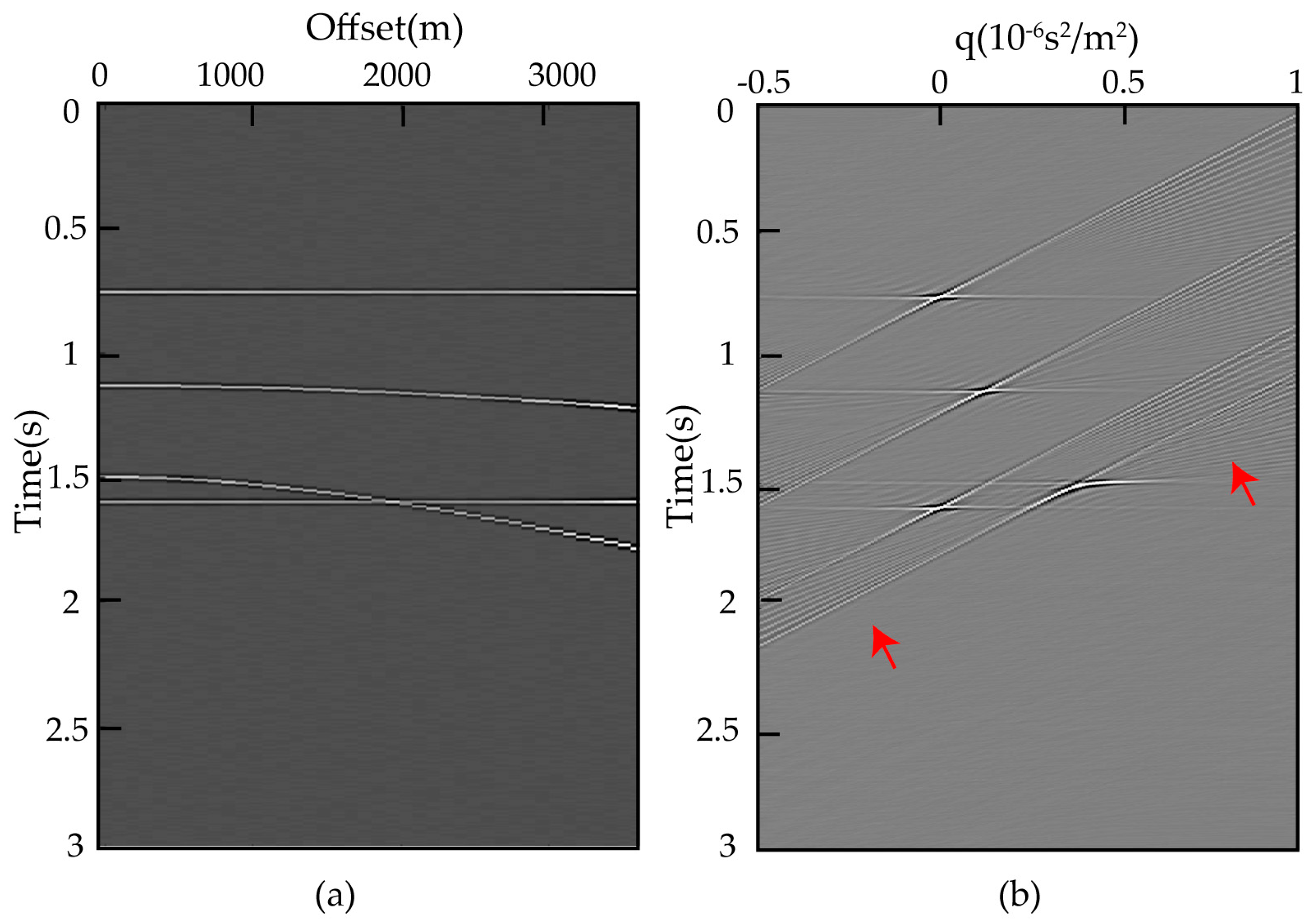
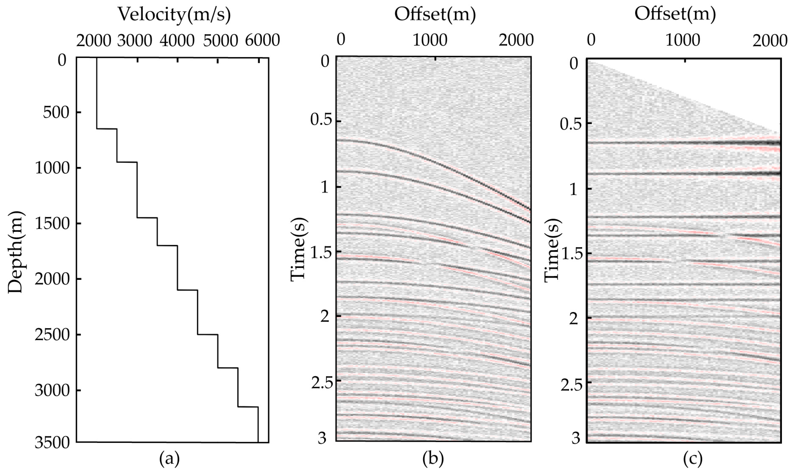
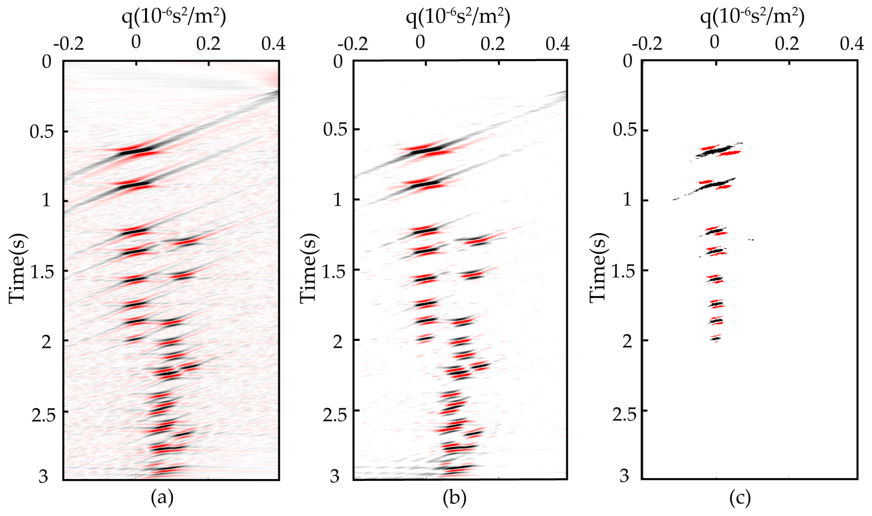
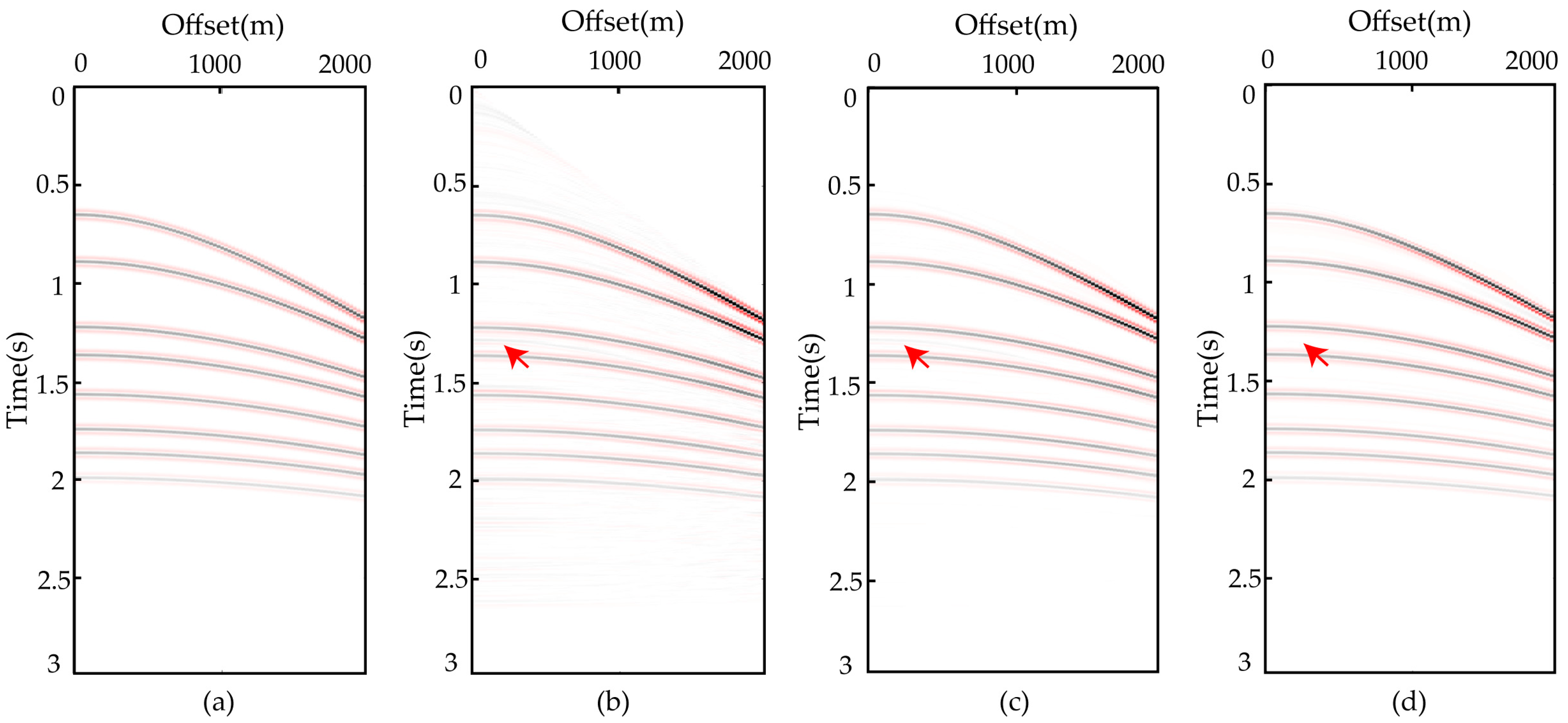
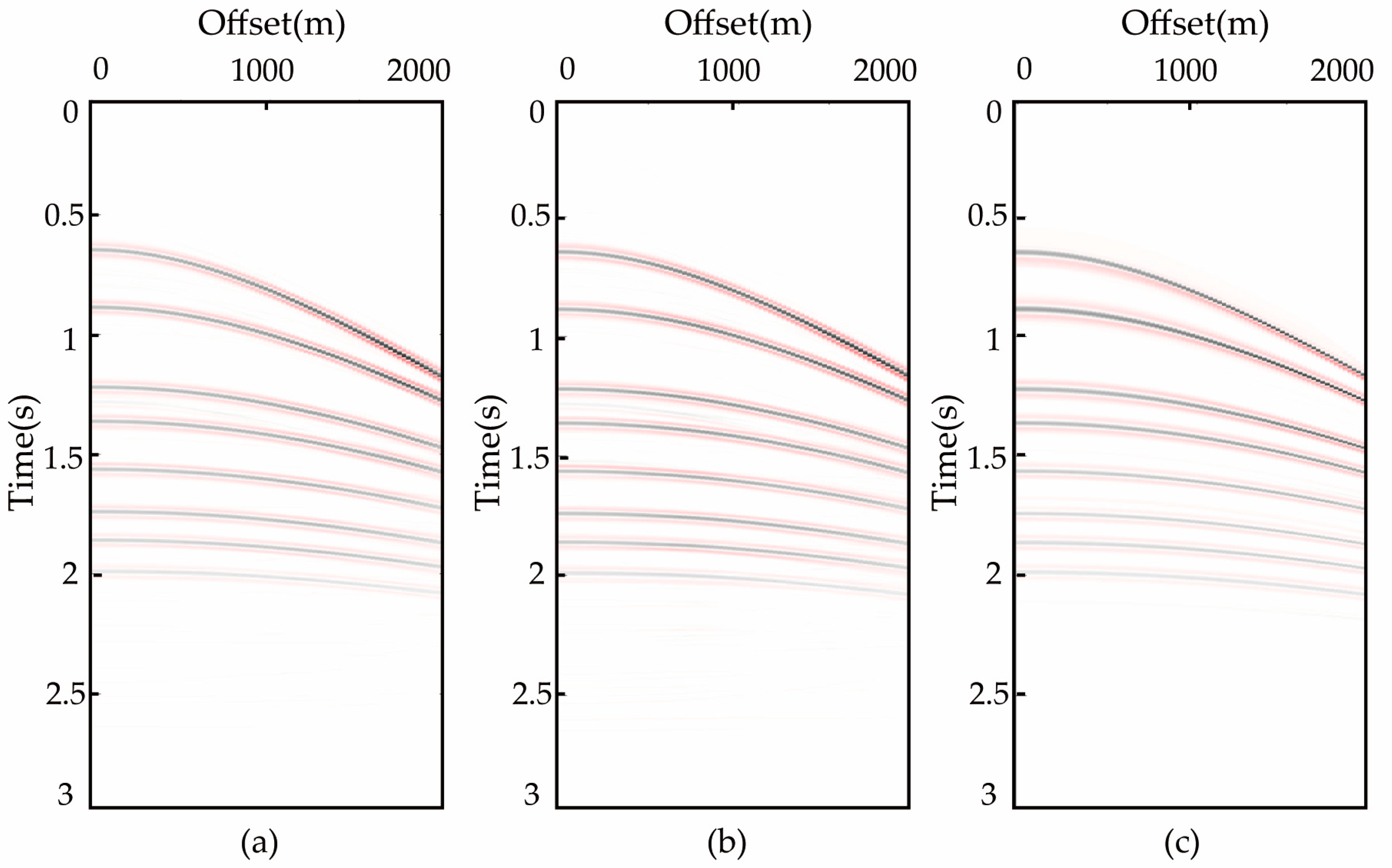
3. Synthetic Data Application

To validate the effectiveness of the proposed method (SPRT$L_{q_1}-L_{q_2}$), we used least squares parabolic Radon transform (LSPRT) and sparse parabolic Radon transform based on $L_1$ regularization (SPRT$L_1$) as the control group to perform a multiple attenuation test on the noisy synthetic data. The velocity model of the synthetic seismic data is shown in Figure 3a. Figure 3b is the CMP gather of a full wavefield. There are 750 sampling points in the time direction, the sampling interval is 4 ms and the offset range is 0 to 2000 m with an interval dx = 25 m.

In order to make the kinematic characteristics of seismic events closer to parabolas, the CMP gather should be normal movement corrected first. The primary reflections are flat and multiple reflections, which are parabolic because of inadequate correction after normal movement correction with velocities of the primary reflections in the CMP gather, as shown in Figure 3c.

After the Radon transform, the seismic events of primaries are mapped in the region with a negative q value and q = 0, and the seismic events of multiples are mapped in the region with a positive q value, as shown in Figure 4. In Figure 4a, due to the influence of the noise, the seismic events do not converge to a point well in the Radon domain, and finite seismic acquisition aperture causes severe smearing. In Figure 4b, although the smearing is alleviated, the result fell short. Figure 4c shows the result of the SPRT$L_{q_1}-L_{q_2}$ method. Because the primary and multiple reflections are sparsely constrained, respectively, only the results of the primary seismic events are left in the Radon domain, and the mapping of multiples is removed directly. There is almost no smearing in Figure 4c, and it has higher resolution. The transformation accuracy and focusing ability are improved.

Figure 5b is the multiple attenuation result obtained by LSPRT; Figure 5c is the result obtained by SPRT$L_1$. Due to the overlapping energy of multiple and primary reflections in the Radon domain, there are many artifacts at near offset. They still have some residual multiple energy, especially at near offset. Figure 5d is the result obtained by SPRT$L_{q_1}-L_{q_2}$. There are almost no residual multiples at the arrow, and the reconstructed data have great consistency with the original data. Figure 6 shows the difference between the suppression results and those without multiple wavefield data. It is proved that the SPRT$L_{q_1}-L_{q_2}$ method is effective in suppressing multiples, especially at the near-offset position. In order to quantitatively analyze the consistency between the reconstructed data and the original data, the following formula is applied to calculate the reconstruction error [42]:

$$s=\frac{{‖m^{\prime }-\widehat{m}‖}_2^2}{{‖m^{\prime }‖}_2^2}\times 100\%$$

(26)

where $m^{\prime }$ is no multiple wavefield data, $\widehat{m}$ is data after multiple attenuation and s is reconstruction error.

Based on the examples of synthetic data,

Table 1. Reconstruction error comparison.

Method	LSPRT	SPRTL1	SPRTLq1 − Lq2
Reconstruction error	11.2%	8.3%	7.6%

lists the reconstruction error of three methods. It is obvious that compared with the LSPRT and SPRT$L_1$ methods, the SPRTL_q1 − L_q2 method is superior in reconstruction capability.

In order to verify whether the proposed method is suitable for seismic data with missing traces, we randomly selected 30%, 50% and 70% seismic trace from the synthetic seismic record containing noise and filled them with zero. We applied the proposed method to suppress multiples of missing seismic trace data. As can be seen from Figure 7a,b, the result of suppressing multiples is not affected, and there are also no residual multiples at the near offset. With the increase in the percentage of missing traces, the reconstruction effect becomes worse. When the percentage of missing traces reaches 70%, the phase distortion appears in the suppression result. Based on the reconstruction results, it can be proved that the SPRT$L_{q_1}-L_{q_2}$ method is also suitable for missing trace data.

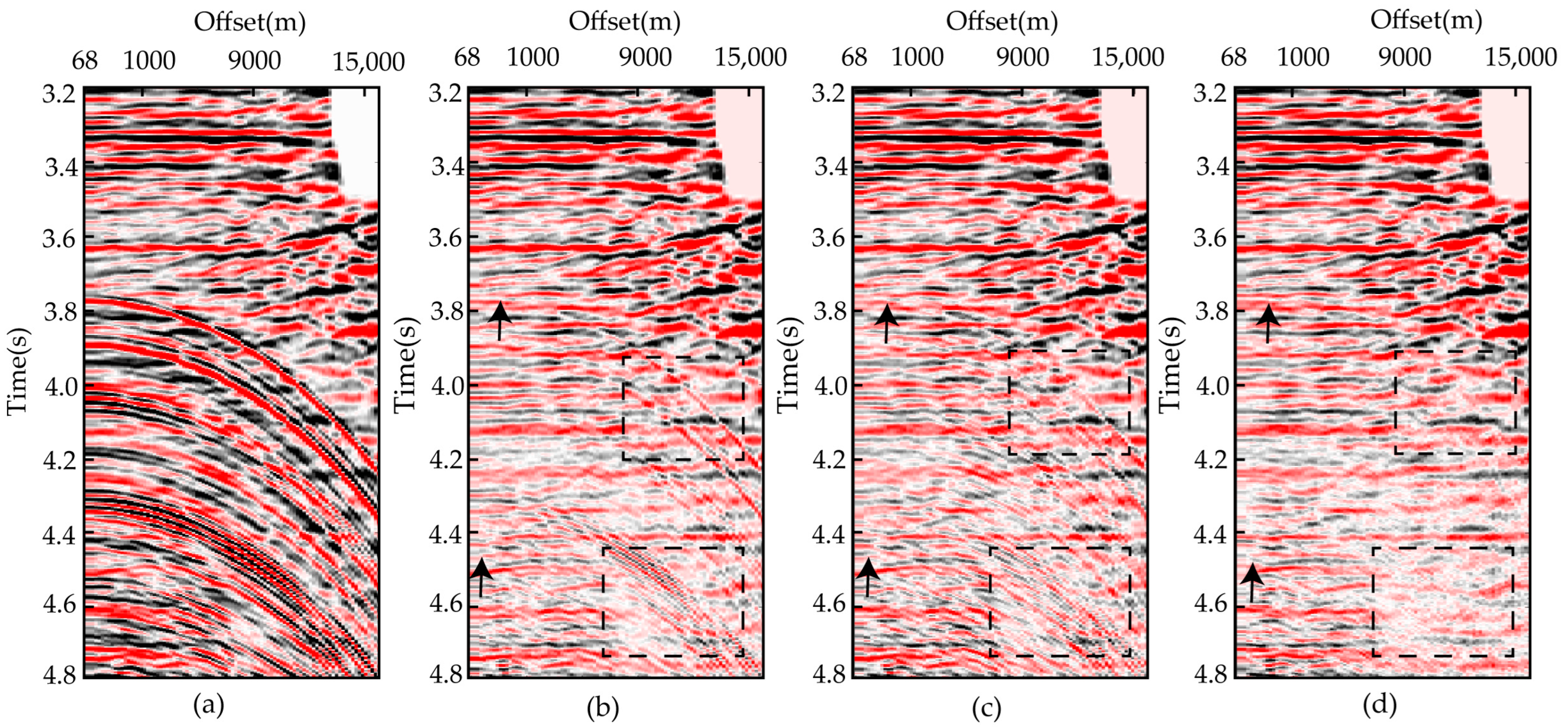
4. Real Data Application

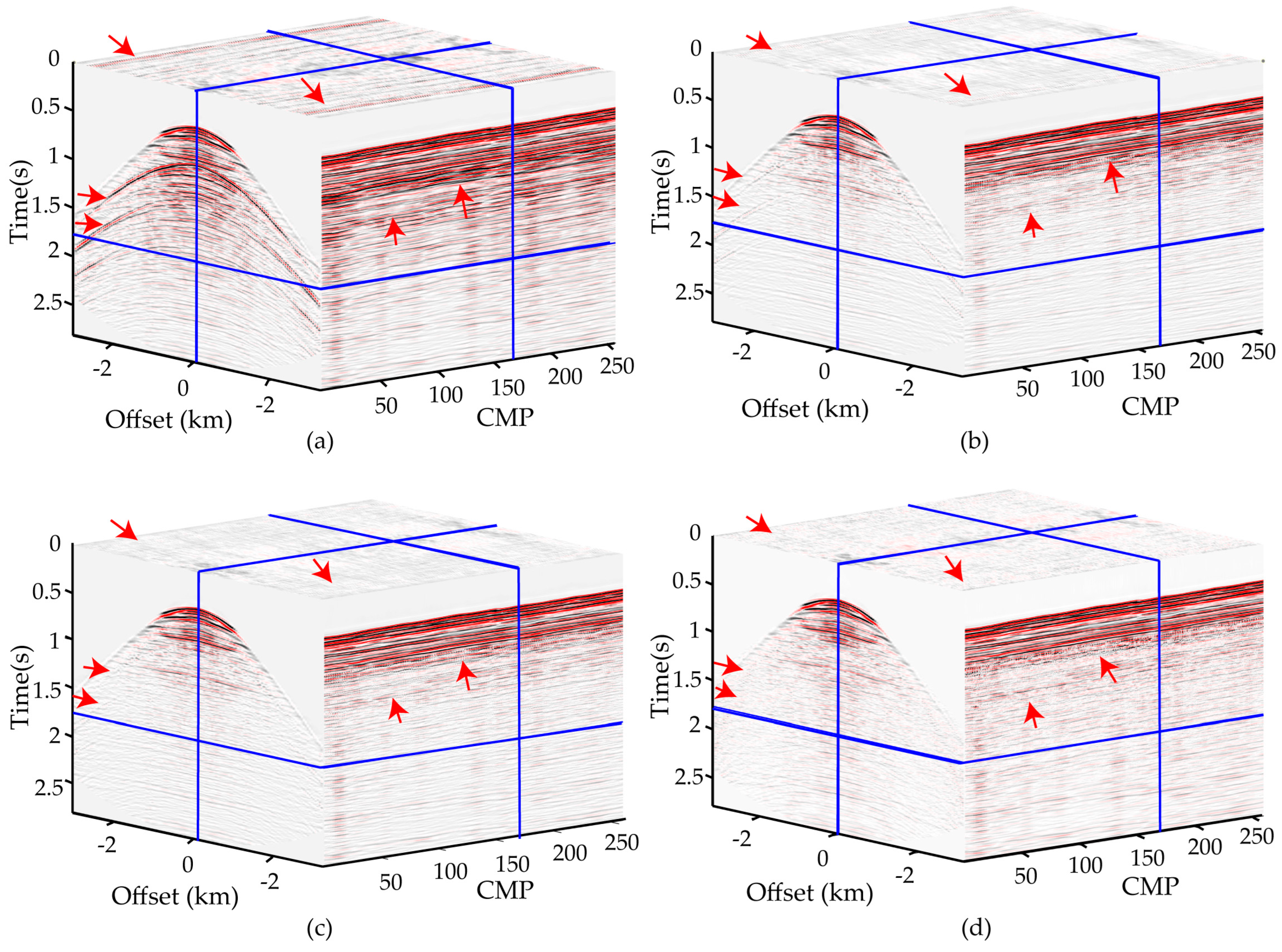
4.1. CMP Gather of Real Data Application

A marine CMP gather after normal movement correction was applied to further examine the effectiveness of the SPRT$L_{q_1}-L_{q_2}$ method. We chose the time window of 3.2 s–4.8 s in the field data to process because there exists a large number of multiple reflections, as shown in Figure 8a. The reason is that this part of the data has more developed multiple waves, and the effect of suppression can be clearly seen in the final result. There are 400 sampling points in the time direction and 92 offset traces. The sampling interval is 4 ms. In addition, those multiple reflections cover the primary data and affect the imaging effect of the primary reflections.

Figure 8 is the multiple attenuation results. Figure 8b,c show the multiple attenuation results of the LSPRT and SPRT$L_1$, and there are still some residual multiple reflections, as indicated by the rectangle. The information of the primaries is masked, and it makes the seismic events discontinuous. Shown in Figure 8d is the multiple attenuation result obtained by SPRTL_q1 − L_q2, and there are no obvious residual multiples. Because of the sparsity of SPRTL_q1 − L_q2, the multiples are suppressed effectively at both near and far offsets. The primaries are highlighted, and the black arrows indicate that the continuity of the seismic events are improved. In addition, we can obviously see that the CMP gather is clear and clean.

In order to further compare the advantages of the proposed algorithm with respect to the LSPRT and SPRT$L_1$, we extracted three single trace amplitudes after multiple attenuation, and they were compared with single-channel amplitudes before suppression. As shown in Figure 9, there is almost no disturbance in the original location of multiples after multiple attenuation by SPRTL_q1 − L_q2, and it is obvious at 4.4 s–4.6 s, and the red rectangle marks the difference in this location. The amplitude of the primary reflection is intact and not attenuated, as at 3.4 s and 3.6 s. The proposed method is effective in suppressing multiples and achieves a better performance.

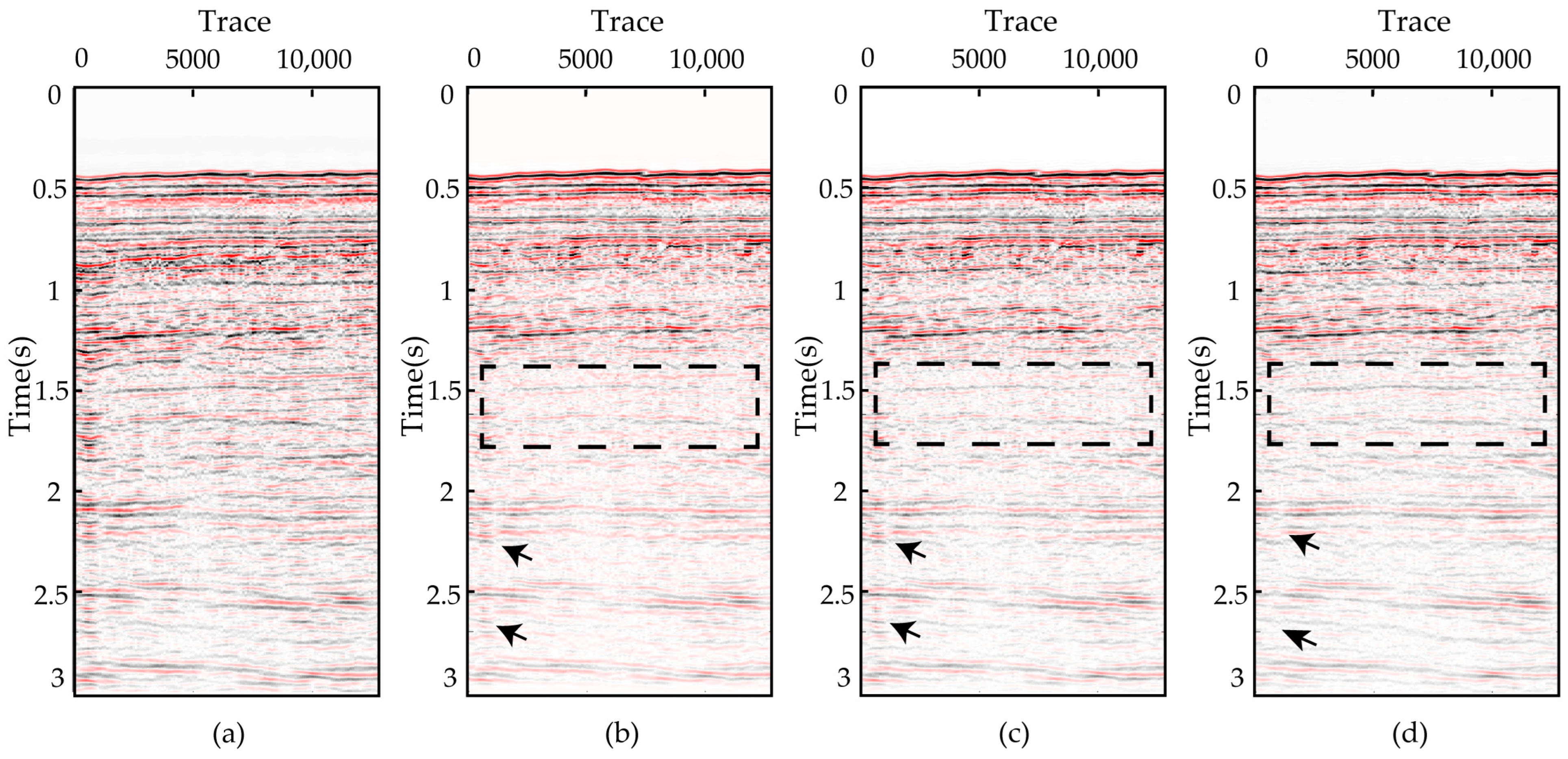
4.2. Prestack Field Data

The SPRTL_q1 − L_q2 method was further tested with multi-shot prestack field data. In order to comprehensively evaluate the multiple suppression effect, we used a 3D method to display the multi-shot data volume, then analyzed the effectiveness of the method from the time slices, the common middle point gathers and the common offset gathers.

Figure 10a is original data, and multiples can be clearly seen at the arrow position in the figure. Figure 10b,c are the multiple attenuation results obtained by the LSPRT and the SPRT$L_1$ methods; Figure 10d is the result obtained by the SPRTL_q1 − L_q2. Overall, all three methods suppress multiples, but the effects are different. In Figure 10b,c, it can be obviously observed from the time slice that a certain amount of the primary energy is lost when multiples are suppressed. In the CMP gathers the multiples of far offset are sufficiently suppressed by SPRTL_q1 − L_q2, as indicated by the arrow. In the common offset gathers, the effectiveness of the SPRTL_q1 − L_q2 method is demonstrated by the continuity of the seismic events. This method has a sparser representation of the seismic data and fully retains the characteristics and information of the primaries, so as to improve the continuity of the seismic events.

Figure 11 shows the stack section after multiple attenuation by three methods. The residual of multiples leads to the discontinuity of the events of the primaries (black rectangle), which increases the difficulty of subsequent interpretation. The continuity of the seismic events is obviously enhanced in the stack sections using the method presented in this paper, and the effect of multiple attenuation between 0.5 s and 1 s has a remarkable effect. In addition, as can be seen by the black arrow region of Figure 11d, there is almost no multiple energy compared to Figure 11b,c.

Therefore, the SPRTL_q1 − L_q2 method has some advantages in suppressing multiple reflections and retaining effective reflections.

5. Discussion

Multiple attenuation can provide a good foundation for subsequent data processing and data interpretation. The traditional parabolic Radon transform is unable to separate primaries and multiples without distortion. Sparse parabolic Radon transform based on $L_1$ regularization also does not achieve the desired effect of suppressing multiples. We introduce the nonconvex $L_{q_1}-L_{q_2}(0<q_1,q_2<1)$ mixed regularization sparse inversion method. This method obviously improves the accuracy of inversion, suppresses multiples and obtains clean seismic data. Moreover, the reconstructed primary data have higher accuracy, which was verified by experimental data.

In this paper, $L_{1/2}$ regularization is used to constrain primary and multiple waves because it has many properties such as sparsity and unbiasedness and oracle properties [25]. Meanwhile, it is more stable and sparse than the $L_1$ regularization, and easier to solve than $L_0$ regularization. In other practical applications, the values of $q_1$ and $q_2$ can be selected according to the actual problem. For example, if the coefficients are not strictly sparse, a moderate to large value of $q$ can yield better results [34].

In complex geological conditions, the weak effective signals in the wavefield are easily covered by noise. Therefore, the parameter setting needs to be more careful, otherwise it may lose an effective signal because of noise suppression.

Since the proposed method introduced the $L_{1/2}$-norm, the computation time is increased when the sparsity of seismic signals is improved. Therefore, the computational efficiency of this method has no advantage over the $L_1$-norm sparse inversion method.

In future research, we propose three research directions that can be improved:

• To solve the problem of the destruction of amplitude versus offset (AVO) signature in seismic data, the proposed method is combined with the orthogonal polynomial transform.
• The algorithm for solving nonconvex regularization is further improved to improve the computational efficiency.
• The proposed method is combined with other multi-wave suppression methods to process seismic data with high efficiency and high quality under complex geological conditions.
• In addition, with the rapid development of deep learning, fields such as mechanics, medicine and geophysics [43,44,45] have been actively combined with deep learning, and more possibilities have been developed. Therefore, in future studies, we will also combine multiple suppression with deep learning to solve problems such as computational efficiency.

6. Conclusions

Multiple attenuation is an important problem in seismic data processing. The suppression results directly affect the quality of stacked seismic data. Radon transform is an efficient and low-cost method. In order to solve the problem of low resolution of Radon transform, a sparse parabolic Radon transform in the frequency domain with the nonconvex $L_{q_1}-L_{q_2}(0<q_1,q_2<1)$ mixed regularization is proposed. This method has higher sparsity, and it can restrict primaries and multiples, respectively. The mappings of multiple seismic events are muted directly in the Radon domain. The theoretical data and field data results show that the resolution of the parabolic Radon transform and reconstruction capability are improved when using SPRT$L_{q_1}-L_{q_2}$($q_1=q_2=1/2$), especially at near offset. The effectiveness of the sparse constraint method is demonstrated in the aspect of seismic event continuity. This method greatly improves the effect of multiple attenuation and reduces the unnecessary energy loss of useful signals, which provides high-quality data for the subsequent primary imaging.

The proposed method can also be used in other processing methods, such as data reconstruction, interpolation and dispersion curve extraction.

References

1. Weglein, A.B. Multiple attenuation: An overview of recent advances and the road ahead. Lead. Edge 1999, 18, 40–44. [Google Scholar] [CrossRef]
2. Verschuuur, D.J. Seismic Multiple Removal Techniques: Past, Present and Future, 1st ed.; Chen, H., Zhang, B., Liu, J., Eds.; Petroleum Industry Press: Beijing, China, 2010; pp. 20–28. [Google Scholar]
3. Wang, X.; Wang, H. A research of high-resolution plane-wave decomposition based on compressed sensing. Chin. J. Geophys. 2014, 52, 1068–1077. [Google Scholar] [CrossRef]
4. Li, Z.N.; Li, Z.C.; Wang, P. Wavefield separation by a modified linear Radon transform in borehole seismic. Chin. J. Geophys. 2014, 57, 2269–2277. [Google Scholar]
5. Zhang, J.; Wang, D.; Hu, B.; Gong, X. An Automatic Velocity Analysis Method for Seismic Data-Containing Multiples. Remote Sens. 2022, 14, 5428. [Google Scholar] [CrossRef]
6. Hampson, D. Inverse velocity stacking for multiple elimination. In SEG Technical Program Expanded Abstracts; Society of Exploration Geophysicists: Houston, TX, USA, 1986. [Google Scholar] [CrossRef]
7. Goncharov, F.O. An Iterative Inversion of Weighted Radon Transforms along Hyperplanes. Inverse Probl. 2017, 33, 124005. [Google Scholar] [CrossRef] [Green Version]
8. Ambartsoumian, G.; Goula-Zarrad, R.; Lewis, M.A. Inversion of the Circular Radon Transform on an Annulus. Inverse Probl. 2010, 26, 11. [Google Scholar] [CrossRef] [Green Version]
9. Thorson, J.R.; Claerbout, J.F. Velocity-stack and slant-stack stochastic inversion. Geophysics 1985, 50, 2727–2741. [Google Scholar] [CrossRef]
10. Sacchi, M.D.; Ulrych, T.J. High-resolution velocity gather and offset space reconstruction. Geophysics 1995, 60, 1169–1177. [Google Scholar] [CrossRef]
11. Herrmann, P.; Mojesky, T.; Magesan, M.; Hugonnet, P. De-aliased, high-resolution Radon transforms. In Proceedings of the 70th Annual International Meeting, SEG, Calgary, AB, Canada, 6–11 August 2000; pp. 1953–1956. [Google Scholar] [CrossRef]
12. Trad, D.; Ulrych, T.; Sacchi, M. Latest views of the sparse Radon transform. Geophysics 2003, 68, 386–399. [Google Scholar] [CrossRef] [Green Version]
13. Lu, W. An accelerated sparse time-invariant Radon trans-form in the mixed frequency-time domain based on iterative 2D model shrinkage. Geophysics 2013, 78, V147–V155. [Google Scholar] [CrossRef]
14. Xiong, F.S.; Huang, X.W.; Zhang, D.; Li, R.; Wang, P. Adaptive multiple subtraction method based on hybrid L1/L2 norm. Geophys. Geochem. Explor. 2014, 38, 996–1002. [Google Scholar] [CrossRef]
15. Chen, S.S.; Donoho, D.L.; Saunders, M.A. Atomic decomposition by basis pursuit. SIAM Rev. 2001, 20, 33–61. [Google Scholar] [CrossRef] [Green Version]
16. Figueiredo, M.A.; Nowak, R.D.; Wright, S.J. Gradient projection for sparse reconstruction: Application to compressed sensing and other inverse problems. IEEE J. Sel. Top. Signal Process. 2007, 1, 586–597. [Google Scholar] [CrossRef] [Green Version]
17. Xue, Y.R.; Wang, M.; Chen, X.H. High resolution Radon transform based on SL0 and its application in data reconstruction. Oil Geophys. Prospect. 2018, 53, 1–7. [Google Scholar] [CrossRef]
18. Tibshirani, R. Regression shrinkage and selection via the Lasso: A retrospective. J. R. Statist. Soc. B 2011, 73, 273–282. [Google Scholar] [CrossRef]
19. Han, J.; Zhang, S.; Zheng, S.; Wang, M.; Ding, H.; Yan, Q. Bias Analysis and Correction for III-Posed Inversion Problem with Sparsity Regularization Based on L1 Norm for Azimuth Super-Resolution of Radar Forward-Looking Imaging. Remote Sens. 2022, 14, 5792. [Google Scholar] [CrossRef]
20. Donoho, D.L. Compressed sensing. IEEE Trans. Inf. Theory 2006, 52, 1289–1306. [Google Scholar] [CrossRef]
21. Chartrand, R.; Staneva, V. Restricted isometry properties and nonconvex compressive sensing. Inverse Probl. 2008, 24, 657–682. [Google Scholar] [CrossRef] [Green Version]
22. Foucart, S.; Lai, M.J. Sparsest solutions of underdetermined linear systems via Lp-minimization for 0 < q ≤ 1. Appl. Comput. Harmon. Anal. 2009, 26, 395–407. [Google Scholar] [CrossRef] [Green Version]
23. Lai, M.J.; Xu, Y.; Yin, W. Improved iteratively reweighted least squares for unconstrained smoothed Lq minimization. SIAM J. Numer. Anal. 2013, 51, 927–957. [Google Scholar] [CrossRef] [Green Version]
24. Marjanovic, G.; Solo, V. Lp Sparsity penalized linear regression with cyclic descent. IEEE Trans. Signal Process. 2014, 62, 1464–1475. [Google Scholar] [CrossRef]
25. Xu, Z.; Zhang, H.; Wang, Y.; Chang, X.; Liang, Y. L1/2 regularization. Sci. China Inf. Sci. 2010, 53, 1159–1169. [Google Scholar] [CrossRef] [Green Version]
26. Chartrand, R.; Yin, W. Iteratively reweighted algorithms for compressive sensing. In Proceedings of the 2008 IEEE International Conference on Acoustics, Speech and Signal Processing, Las Vegas, NV, USA, 31 March–4 April 2008; pp. 3869C–3872C. [Google Scholar] [CrossRef]
27. Xu, Z.; Chang, X.; Xu, F.; Zhang, H. L1/2 Regularization: A Thresholding Representation Theory and a Fast Solver. IEEE Trans. Neural Netw. Learn. Syst. 2012, 23, 1013–1027. [Google Scholar] [CrossRef] [PubMed]
28. Zuo, W.; Meng, D.; Zhang, L.; Feng, X.; Zhang, D. A Generalized Iterated Shrinkage Algorithm for Non-convex Sparse Coding. In Proceedings of the IEEE International Conference on Computer Vision, Sydney, Australia, 1–8 December 2013; pp. 217–224. [Google Scholar] [CrossRef] [Green Version]
29. Li, Y. Research on image recovery technology via nonconvex regularization method. Ph.D. Thesis, Nanjing University of Posta and Telecommunications, Nanjing, China, 2020. [Google Scholar] [CrossRef]
30. Huang, S.; Xu, Y.; Ren, M.; Yang, Y.; Wan, W. Rain Removal of Single Image Based on Directional Gradient Priors. Appl. Sci. 2022, 12, 1628. [Google Scholar] [CrossRef]
31. Wang, R.; Wang, D.; Zhang, W.; Liu, Y.; Hu, B.; Wang, L. Pseudo-3D Receiver Deghosting of Seismic Streamer Data Based on I1 Norm Sparse Inversion. Appl. Sci. 2022, 12, 556. [Google Scholar] [CrossRef]
32. Zhang, H.; Chen, J. Robust Lp-Norm Inversion for High-Resolution Fluid Contents from Nuclear Magnetic Resonance Measurements. Appl. Sci. 2021, 11, 1298. [Google Scholar] [CrossRef]
33. Chen, J.; Zhang, Z.; Wen, X. Target Identification via Multi-View Multi-Task Joint Sparse Representation. Appl. Sci. 2022, 12, 955. [Google Scholar] [CrossRef]
34. Wen, F.; Lasith, A.; Pei, L.; Roummel, F.M.; Liu, P.; Robert, C.Q. Nonconvex Regularization-Based Sparse Recovery and Demixing with Application to Color Image Inpainting. IEEE Access 2017, 5, 11513–11527. [Google Scholar] [CrossRef]
35. Wen, F.; Pei, L.; Yang, Y.; Yu, W.; Liu, P. Efficient and Robust Recovery of Sparse Signal and Image using Generalized Nonconvex Regularization. IEEE Trans. Comput. Imaging 2017, 3, 566–579. [Google Scholar] [CrossRef] [Green Version]
36. Mei, J.; Xi, J. Efficient Sparse Recovery and Demixing using Nonconvex Regularization. IEEE Access 2019, 7, 59771–59779. [Google Scholar] [CrossRef]
37. Dykes, L.; Huang, G.X.; Silvia Noschese, S.; Reichel, L. Regularization Matrices for Discrete ill-posed Problems in several Space Dimensions. Numer. Linear Algebr. Appl. 2018, 25, 1. [Google Scholar] [CrossRef] [Green Version]
38. Daubechies, I.; Defrise, M.; De Mol, C. An iterative thresholding algorithm for linear inverse problems with a sparsity constraint. Commun. Pure Appl. Math. 2004, 57, 1413–1457. [Google Scholar] [CrossRef] [Green Version]
39. Beck, A.; Teboulle, M.A. fast iterative shrinkage-thresholding algorithm for linear inverse problems. SIAM J. Imaging Sci. 2009, 2, 183–220. [Google Scholar] [CrossRef] [Green Version]
40. Boyd, S.; Parikh, N.; Chu, E.; Peleato, B.; Eckstein, J. Distributed optimization and statistical learning via the alternating direction method of multipliers. Found. Trends Mach. Learn. 2011, 3, 1–122. [Google Scholar] [CrossRef]
41. Marjanovic, G.; Solo, V. On lq optimization and matrix completion. IEEE Trans. Signal Process. 2012, 60, 5714–5724. [Google Scholar] [CrossRef]
42. Duan, S.Y.; Yang, B.T.; Wang, F.; Liu, G.R. Determination of Singular Value Truncation Threshold for Regularization in Ill-Posed Problems. Inverse Probl. Sci. Eng. 2021, 29, 1127–1157. [Google Scholar] [CrossRef]
43. Biousse, V.; Danesh-Meyer, H.V.; Saindane, A.M.; Lamirel, C.; Newman, N.J. Imaging of the Optic Nerve: Technological Advances and Future Prospects. Lancet Neurol. 2022, 21, 1135–1150. [Google Scholar] [CrossRef]
44. Soleimani-Babakamali, M.H.; Sepasdar, R.; Nasrollahzadeh, K.; Sarlo, R. A system reliability approach to real-time unsupervised structural health monitoring without prior information. Mech. Syst. Signal Proc. 2022, 171, 108913. [Google Scholar] [CrossRef]
45. Shotaro, N.; Gerrit, B. Machine-Learning-Based Data Recovery and Its Contribution to Seismic Acquisition: Simultaneous Application of Deblending, Trace Reconstruction, and Low-Frequency Extrapolation. Geophysics 2021, 86, 13–24. [Google Scholar] [CrossRef]
Figure 1. (a) CMP gather after NMO; (b) Radon domain data after parabolic Radon transform. The red arrows indicate the smearing.
Applsci 13 02550 g001
Figure 2. Unit ball pictures for (a) L0, (b) L2, (c) L1 and (d) L1/2 regularization.
Applsci 13 02550 g002
Figure 3. (a) Velocity model; (b) CMP gather; (c) CMP gather after NMO.
Applsci 13 02550 g003
Figure 4. Radon domain results: (a) LSPRT method; (b) SPRTL1 method; (c) SPRTLq1Lq2 method.
Applsci 13 02550 g004
Figure 5. Multiple attenuation result of the theoretical model data: (a) without multiple wavefield data; (b) LSPRT method; (c) SPRT L 1  method; (d) SPRTLq1Lq2 method. The red arrows indicate the multiples suppression effect of the three algorithms, and there is no residual multiples in Figure 5d.
Applsci 13 02550 g005
Figure 6. Difference image map: (a) by LSPRT; (b) by SPRTL1; (c) by SPRTLq1Lq2.
Applsci 13 02550 g006
Figure 7. Multiple attenuation results of missing trace data by SPRTLq1Lq2: (a) 30% missing traces; (b) 50% missing traces; (c) 70% missing traces.
Applsci 13 02550 g007
Figure 8. Multiple attenuation result: (a) CMP gather of marine real data; (b) by LSPRT method; (c) by SPRTL1 method; (d) by SPRTLq1Lq2 method. The black arrows indicate the continuity of the seismic events are improved in the Figure 8d.
Applsci 13 02550 g008
Figure 9. Comparison of single trace amplitude after multiple attenuation by three algorithms. The red rectangle indicate that the amplitude of multiple decays more significantly in the proposed method.
Applsci 13 02550 g009
Figure 10. Multiple attenuation result: (a) pre-stack real data; (b) LSPRT method; (c) SPRTL1 method; (d) SPRTLq1Lq2 method. The red arrows indicate the cleaner multiple attenuation in the Figure 10d.
Applsci 13 02550 g010
Figure 11. Multiple attenuation result: (a) stacked real data; (b) LSPRT method; (c) SPRTL1 method; (d) SPRTLq1Lq2 method. The black arrows indicate the continuity of the seismic events are improved in the Figure 11d.
Applsci 13 02550 g011