Featured Application
This paper employs intelligent methods to forecast ground settlement caused by tunnel construction in order to provide a solid foundation for risk warning and risk management.
Abstract
Construction-induced ground settlement is a serious hazard in underground tunnel construction. Accurate ground settlement prediction has great significance in ensuring the surface building’s stability and human safety. To that end, 148 sets of data were collected from the Singapore Circle Line rail traffic project containing seven defining parameters to create a database for predicting ground settlement. These parameters are the tunnel depth (H), the tunnel advance rate (AR), the EPB earth pressure (EP), the mean SPTN value from the soil crown to the surface (Sm), the mean water content of the soil layer (MC), the mean modulus of elasticity of the soil layer (E), and the grout pressure used for injecting grout into the tail void (GP). Three hybrid models consisting of random forest (RF) and three types of meta-heuristics, Ant Lion Optimizier (ALO), Multi-Verse Optimizer (MVO), and Grasshopper Optimization Algorithm (GOA), were developed to predict ground settlement. Furthermore, the mean absolute error (MAE), the mean absolute percentage error (MAPE), the coefficient of determination (R2) and the root mean square error (RMSE) were used to assess predictive performance of the constructed models for predicting ground settlement. The evaluation results demonstrated that the GOA-RF with a population size of 10 has achieved the most outstanding predictive capability with the indices of MAE (Training set: 2.8224; Test set: 2.3507), MAPE (Training set: 40.5629; Test set: 38.5637), R2 (Training set: 0.9487; Test set: 0.9282), and RMSE (Training set: 4.93; Test set: 3.1576). Finally, the sensitivity analysis results indicated that MC, AR, Sm, and GP have a significant impact on ground settlement prediction based on the GOA-RF model.
1. Introduction
Surface traffic cannot meet the development needs of a large city, therefore underground tunnel construction is gradually becoming the primary option for urban transportation projects [1]. Earth pressure balance (EPB) is a common method for underground construction in cities with dense surface buildings. Viewed from the construction perspective, the main construction area of an urban tunnel is concentrated in the soft layer under the dense building group in cities [2]. This will inevitably cause settlement due to the effects of two major factors: shallow depth and soft ground [3,4,5]. Once ground settlement occurs, building safety and other public utilities above the construction area are seriously threatened. Therefore, predicting ground settlement caused by tunneling is an essential part of the risk analysis of urban tunnel projects [6,7,8].
To provide an important foundation for assessing potential risks and adjusting construction plans [9], four methods are commonly used to assess ground settlement caused by tunnel construction, i.e., empirical [10,11], analytical [12], numerical [13,14], and artificial intelligence methods [15,16,17,18]. Although the empirical method has a longer history of application, which not only involves incomplete parameters, it also does not have the best prediction accuracy [19]. Some widely used empirical equations are listed in Table 1. Subsequently, analytical, and numerical simulation methods were used to calculate ground settlement. In most real-world situations, the analytical method struggles to recreate the excavation process during the calculation; as a result, numerous simplifications were applied in the calculation process, leading to biased results [20]. Łodygowski and Sumelka [21] pointed out the shortcomings of numerical simulation methods in terms of timeliness and the problem of considering boundary difficulties. Therefore, avoiding the complex process of reverting tunnel construction in the calculation process and the method of exploring the relationship between numerous weakly correlated parameters becomes a challenge in ground settlement prediction. Table 1 displays a selection of studies pertaining to empirical, analytical, and numerical methods for calculating ground settlement.

Table 1.
The empirical method, analytical method, and numerical method for ground settlement calculation.
Artificial intelligence methods have received focused attention due to the fact that they do not require prior experience as support, as well as having the ability to work with multiple influential variables. Samui [44] introduced a support vector machine (SVM) approach for predicting ground settlement in shallow soils and analyzed the importance of parameters affecting settlement prediction. Nejad et al. [45] found that artificial neural network (ANN) has the better performance for the pile foundation settlement prediction than other conventional artificial intelligence methods. Moreover, artificial intelligence techniques have been implemented in a vast array of fields [46,47,48,49,50,51]. Table 2 displays the application of different artificial intelligence methods to ground settlement prediction.
Table 2.
Intelligent method for ground settlement prediction.
However, numerous shortcomings of some intelligent methods are gradually revealed in practical application. For example, it is difficult to determine the network structure of ANN models and have poor generalization performance [18]. SVM also has practical issues, such as high model complexity and significant limitations in kernel functions [18]. As a consequence, finding an appropriate prediction method for ground settlement brought on by tunnel excavation remains a critical issue.
Breiman [69] proposed an artificial intelligence approach called RF, which is an integrated model combining of tree predictors. This model has good generalization and is more robust in terms of noise control. Numerous scholars revealed the advantages of RF models in the field of geotechnical and tunneling engineering [70,71,72,73,74,75,76,77,78,79]. Dong et al. [80] compared the classification performance of ANN, SVM and RF models for predicting the rockburst intensity. The results showed that the misclassification rates of these models are 0.1, 0.2, and 0, respectively. Tao et al. [81] conducted a study on predicting the tunnel boring machine (TBM) penetration rate. The results showed that the RF regression algorithm has achieved a high accuracy prediction of the mean squared error (MSE) at 0.0504. Zhou et al. [18] investigated the geometric, geological, and operational parameters as input variables to train RF models for the ground settlement prediction. A good prediction accuracy has been achieved by means of valuable performance indices (R2: 0.93, RMSE: 15). However, few RF models with particularly good results were developed to predicting ground settlement during tunnel excavation. Motivated by the above considerations, the main goal of this paper is to establish some hybrid RF models based on the three types of meta-heuristics named, Ant Lion Optimizer (ALO), Multi-Verse Optimizer (MVO), and Grasshopper Optimization Algorithm (GOA). In practice, these metaheuristic techniques are meritocratic with regard to the RF hyperparameters and improve the predictive accuracy of the model.
This paper is organized as follows: the RF model and three used meta-heuristic algorithms are introduced in Section 2. Section 3 describes the relevant parameters, four performance evaluation indices and model development (Matlab 2021 was used in this paper to complete the model construction). Subsequently, the performance evaluation results of all hybrid RF models for the ground settlement prediction are displayed and discussed in Section 4. Finally, the main conclusions and limitations of this paper are summarized in Section 5.
2. Materials and Methods
2.1. Random Forest
RF is a class of multi-decision tree integration models previously proposed by Breiman [69]. There are two types of trees in RF, i.e., classification tree and regression tree. The latter is used to solve the regression problem including the ground settlement prediction during tunnel excavation. For the regression RF model, the training performed for each decision tree is based on a separate subset of data, even if a data point in the dataset changes, it only affects one decision tree and hardly affects all of them [82]. This is one of the reasons why the RF model is resistant to overfitting. The framework of RF regression can be represented by the following [69]:
- Multiple training sets are randomly generated using the Bootstrap resampling method.
- Each training subset generates a decision tree that will be split in an optimal way in a randomly selected set of attributes. The tree will grow to its maximum without being pruned.
- The above steps were repeated until the number of regression trees reached the upper limit set by the researchers.
2.2. Ant Lion Optimizier (ALO)
The Ant Lion Optimization (ALO) algorithm is a meta-heuristic approach proposed by Mirjalili [83] to solve the optimization problem. This algorithm was inspired by the predation strategy of ant lions. Ant lions in nature are good at building funnel-shaped traps to capture ants who fall into their traps. The ALO optimization algorithm simulates the predation strategy of ant lions to search for the optimal solution. The algorithm consists of five steps: simulating the random movement of ants, preparing the trap, trapping the ants, feeding, and reconfiguring the trap.
The irregular actions of ants in the search for food can be represented in the algorithm by the following equations:
where G(l) is the set of steps for ants to wander randomly, csm represents the cumulative sum, n represents the maximum number of iterations, l shows the step length of the ant movement (the current iteration in the algorithm), and r(l) is a random function, rand denotes a random number in the range of [0,1].
Because the traps laid by the ant lion affect the random movement of the ants, the algorithm restricts the movement of the ants is restricted in the range of a certain sphere of ant lion. To better simulate the survival of the fittest in nature, the roulette strategy was used to give more adaptable ant lions chance to catch ants. Based on this strategy, the ant lions can build traps that match adaptive scale. When ants fall into the trap, their movement range is adaptively reduced to constantly approach the ant lion’s position. After a successful predation, the ant lion updated its position to the prey position to improve the success of subsequent hunting. Its location is updated as follows:
where Alj represents the position of the j-th ant at the l-th iteration and ALli represents the updated position of the i-th ant lion at the l-th iteration.
Eventually, the optimal ant lion in each iteration is retained as an elite that can influence the random movement of all ants in the process.
2.3. Multi-Verse Optimizer (MVO)
Multi-Verse Optimization (MVO) is a class of nature-inspired algorithms proposed by Mirjalili [84]. Physicists believe that the Big Bang can be thought of as a white hole and an integral part of the universe; the black hole absorbs all matter, including light; and the wormhole is a tunnel that connects parts of the universe to each other. Therefore, the algorithm is inspired by a cyclic multiverse model [85]: the stability among multiple universes is controlled by an interaction of black holes, white holes, and wormholes.
Moreover, the objects with high expansion rate in the universe (white holes in the algorithm) always tend to move toward the objects with low expansion rate (black holes in the algorithm), and this movement is made possible by wormholes. In the MVO algorithm, wormholes are used as the channel medium to connect white holes and black holes for detecting the search space, as shown in Figure 1.
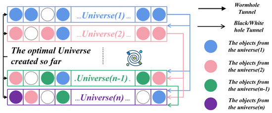
Figure 1.
The schematic diagram of MVO.
The algorithm contains two important parameters: traveling distance rate (TDR) and wormhole existence probability (WEP). The TDR represents the distance an object can travel through a wormhole near the optimal universe and can be expressed as follows:
where q represents the exploration accuracy during the iteration, h represents the current iteration, and H represents the maximum number of iterations.
The WEP expresses the probability of wormhole occurrence and can be expressed by the following equation:
where MAX represents the maximum value (1 in this paper), and MIN represents the minimum value (0.2 in this paper), n is the current iteration, N shows the maximum iterations.
2.4. Grasshopper Optimization Algorithm (GOA)
Saremi et al. [86] proposed the grasshopper optimization algorithm (GOA) to solve optimization problems. This is a class of bionic optimization algorithms that simulates the group behavior of grasshoppers. The algorithm divides the behavioral trends of grasshopper swarms into exploration and exploitation. In the exploration phase, grasshoppers normally move abruptly, while they prefer to move more regionally in the exploitation phase. These two patterns of grasshoppers behavior are modeled mathematically.
The position of the i-th grasshopper is denoted by xi in the algorithm, and the group behavior of the grasshoppers can be expressed by the following equation:
The social definition function g(r) can be expressed as follows:
where ubd and lbd are the upper and lower bounds of the d-dimensional space, respectively, and is the distance between the i-th grasshopper and the j-th grasshopper; is the location vector of the grasshopper target food; f denotes the strength of attraction; c shows the attractive length scale. The reduction of the grasshopper’s comfort zone is captured by the coefficient k:
where kmax represents the maximum (1 in this work) and kmin represents the minimum values (0.00001 in this work), respectively; t is the current iteration, while T represents the maximum iteration.
3. Database Preparation
In this study, the data were collected from the Singapore Circle Line rail traffic project [61,87,88,89]. The projects were constructed with EPB machines and some basic parameters are shown in Table 3. The tunnel was lined with a precast concrete tunnel liner with an internal diameter of 5.8 m. The spacing of the measurement points for ground settlement was about 25 m. After the excavation of each section of the tunnel project was completed, the settlement of that section was measured.
Table 3.
Tunnel project construction parameters.
The construction section contains mainly four different types of soil conditions as shown in Figure 2. The stratigraphic characteristics are systematically described by Goh et al. [61], Hulme and Burchell [87] and Shirlaw et al. [89,90].
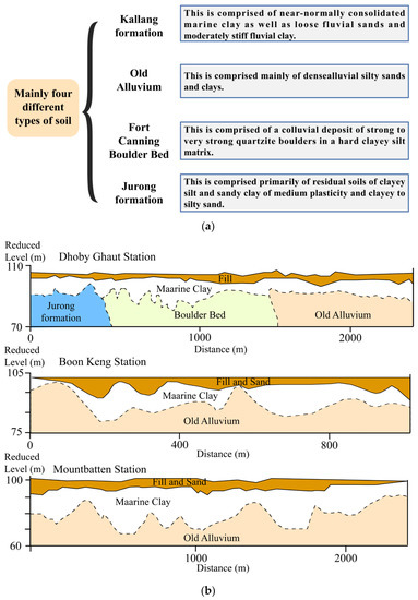
Figure 2.
Soil condition of tunnel engineering: (a) Major soil types in tunneling projects; (b) Longitudinal soil profiles of projects.
3.1. Data Structure
The database contains 148 ground settlement data and other related parameters are represented and described as shown in Figure 3. These parameters affecting ground settlement can be divided into three categories [53,61]: geological conditions, tunnel geometry conditions, and operational parameters.
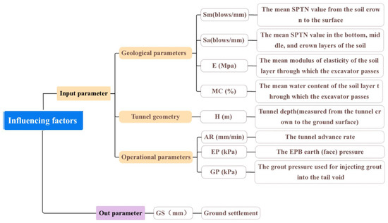
Figure 3.
Introduction of influencing factors related to ground settlement.
The geological parameters included in the database of this study are the mean SPT N (standard penetration test) value from the soil crown to the surface (Sm), the mean SPT N value in the bottom, middle, and crown layers of the soil (Sa), the mean modulus of elasticity of the soil layer (E) and the mean water content of the soil layer (MC). Since the groundwater levels of the three projects are similar, they are not considered to be input variables. The geometric parameters of the tunnels are mainly considered to be the inner diameter and the depth to the surface (H) of the tunnel. Since the inner diameter of the tunnel was the same in all three projects, it was not used as an input variable in this study. The operational parameters of the tunnel that can be used as input parameters for this study are the tunnel advance rate (AR), the EPB earth pressure (EP) and the grout pressure used for injecting grout into the tail void (GP). In addition, the ground settlement (GS) is output parameter in this study.
3.2. Sensitivity Analysis
Parameters sensitivity analysis can help reduce redundancy in the data and improve prediction efficiency. Therefore, the correlation between all parameters of used database is examined using Pearson correlation analysis, and the results are shown in Figure 4.
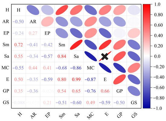
Figure 4.
Pearson correlation coefficient analysis of land subsidence parameters.
As illustrated in Figure 4, it is not difficult to find that the correlation coefficient between E and Sa is high of 0.99. The result indicated that there is an extremely strong correlation between these two parameters, and further analysis reveals that the correlation between the two types of characteristic parameters and the others is similar. Therefore, Sa is not considered to be an input parameter. The correlations between the remaining parameters and GS meets the requirements of the study. Therefore, the input parameters used in this study are H, AR, EP, Sm, MC, E, and GP, and the output parameter is GS.
3.3. Evaluation Indicators
The performance evaluation is a key part for the model construction, which is related to the optimal model selection after finishing prediction [78,91,92]. In this study, four statistical indices named the coefficient of determination (R2), the mean absolute error (MAE), the mean absolute percentage error (MAPE), and the root mean square error (RMSE) were used to evaluate the model performance. The definition and calculation equation of each evaluation index is shown in Table 4.
Table 4.
Definition of evaluation indicators and their calculation.
3.4. Hybrid Models
Hyperparameters have a significant impact on model performance, thus three metaheuristics (ALO, WVO, and GOA) were selected to optimize hyperparameters of RF model in this study. The model constructing process of ALO-RF, WVO-RF and GOA-RF models is shown in Figure 5. The number of populations was set to 10, 20, 50, 100, and the iteration was set to 500 to ensure that all models were fully optimized. One-hundred forty-eight data sets were divided into a training set and a test set in a 3:1 ratio. Furthermore, a five-fold CV approach was used to choose the best optimization parameters for the training set data in order to reduce model overfitting [93,94]. Then, three metaheuristic approaches: ALO, WVO, and GOA, were used to optimize the RF hyperparameters and enhance the accuracy of the model. The MAE, MAPE, RMSE, and R2 were used as evaluation indices to evaluate the predictive capability of ALO-RF, WVO-RF, and GOA-RF models for estimating GS and to determine the optimal model. Finally, the importance of each input parameter was analyzed to grasp the influence of them on GS.
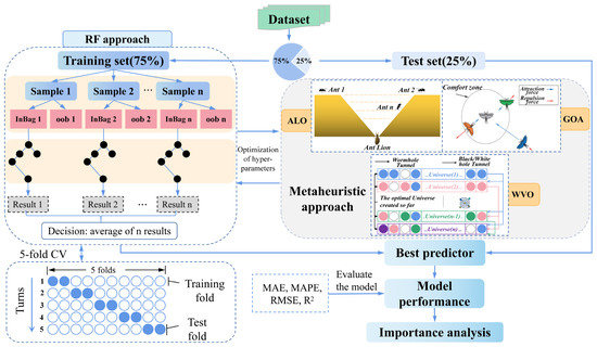
Figure 5.
Flow chart of hybrid models (ALO-RF, WVO-RF and GOA-RF) construction.
4. Discussion
4.1. Model Efficiency Evaluation
With the help of the three-class metaheuristic technique, the predictive ability of the RF model is enhanced, and the ALO-RF, WVO-RF, and GOA-RF hybrid models are obtained. The RMSE was chosen to calculate the fitness values of each developed model. As illustrated in Figure 6, the fitness values of all developed models with different populations had been minimized and stabilized after reaching the maximum number of iterations.

Figure 6.
The iteration curve of each hybrid model: (a) ALO-RF; (b) WVO-RF and (c) GOA-RF; Pop: population).
As can be seen in this picture, it is easy to find that the convergence time of GOA-RF hybrid models with different populations is slightly faster than ALO-RF and WVO -RF models. In conclusion, the variation of the fitness function confirms the effectiveness of the three types of optimization algorithms and visualizes the optimization efficiency of the different algorithms. The predictive performance of the three types of hybrid models for GS is evaluated more fully in Section 4.2.
4.2. Model Prediction Performance Evaluation
To better assess the optimization capability of ALO, WVO and GOA, the unoptimized RF model was introduced to compare predictive performance with three hybrid RF models.
Figure 7 illustrates the total scores of four evaluation indices for each hybrid model. The larger sector area represents a higher score obtained by a model. In other words, the hybrid model has a superior performance than other models for the ground settlement prediction. Figure 7a displays the cumulative scores of ALO-RF models with population sizes of 10, 20, 50, and 100. It can be obviously observed that the ALO-RF model with 10 population obtains the highest cumulative score. This result indicated that the ALO-RF model with 10 is the best model for the GS prediction than other similar models. Similarly, in Figure 7b, the WVO-RF model with a population size of 100 receives the highest score for each evaluated indices, who demonstrates a superior capacity to predict GS. The cumulative score of GOA-RF with a population size of 10 was then greater than other models considering other population sizes, thus it is the best prediction model for forecasting the GS.
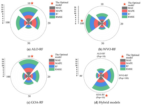
Figure 7.
Hybrid model comprehensive performance evaluation: (a) Comparison of ALO-RF results for populations of 10, 20, 50, 100; (b) Comparison of WVO-RF results for populations of 10, 20, 50, 100; (c) Comparison of GOA-RF results for populations of 10, 20, 50, 100; (d) Comparison of the results of different models.
To better visualize the performance of each ALO-RF, WVO-RF, and GOA-RF models, the relationships between predicted and measured GS values were depicted in Figure 8. Each sphere in this figure represents the distribution of a set of measured and predicted values. If the sphere lies on the diagonal line, the measured value is equal to the predicted value. Moreover, the histogram of differences located in the upper right corner of the figure represents the distribution of differences between predicted and measured values. The proximity of measured values and predicted values by ALO-RF, WVO-RF, and GOA-RF models to the diagonal dashed line indicates that all hybrid models are effective for predicting the GS. By comparison of details, the distribution of GOA-RF (Pop = 10) is more concentrated near the diagonal dashed line than ALO-RF (Pop = 10) and WVO-RF (Pop = 100) models. In the training set, the MAE of GOA-RF model is significantly lower than that of ALO-RF and WVO-RF models (ALO-RF: 2.9516, WVO-RF: 2.865, GOA-RF: 2.8224); the RMSE of GOA-RF model is also the lowest among three models (ALO-RF: 5.4133, WVO-RF: 5.3441, GOA-RF: 4.93); and the R2 value of GOA-RF model is higher than ALO-RF and WVO-RF models (ALO-RF: 0.9338, WVO-RF: 0.9409, GOA-RF: 0.9487); the MAPE of GOA-RF model is similar to the WVO-RF model, which are both at a low level (ALO-RF: 50.5681, WVO-RF: 40.3814, GOA-RF: 40.5629). In the test set, the MAE of GOA-RF model is the lowest among three models (ALO-RF: 2.819, WVO-RF: 2.5786, GOA-RF: 2.3507); similarly, the RMSE of GOA-RF model is also the lowest value (ALO-RF: 3.5978, WVO-RF: 3.2843, GOA-RF: 3.1576); and the R2 of GOA-RF presents is higher than ALO-RF and WVO-RF models (ALO-RF: 0.9055, WVO-RF: 0.9202, GOA-RF: 0.9282); the MAPE of GOA-RF is at a low value as the same as with WVO-RF (ALO-RF: 48.5579, WVO-RF: 38.7341, GOA-RF: 38.7537). This result demonstrated that GOA-RF is the best hybrid model for GS prediction. In the training phase, the error range of all three hybrid models is primarily concentrated within 10 mm, whereas it is concentrated within 8 mm in the testing phase. It is evident that all hybrid models have an effective error control.
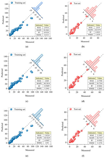
Figure 8.
Distribution of prediction results and histogram of differences based on three hybrid models: (a) ALO-RF(Pop = 10, Train set); (b) ALO-RF(Pop = 10, Test set); (c) WVO-RF(Pop = 100, Train set); (d) WVO-RF(Pop = 100, Test set); (e) GOA-RF(Pop = 10, Train set); (f) GOA-RF(Pop = 10, Test set).
After determining the optimal population size for each hybrid model (ALO-RF, WVO-RF, and GOA-RF), further comparisons were made with the unoptimized RF model. Figure 9 depicts Taylor diagrams for four models and lists the corresponding evaluation indices. Taylor diagrams can demonstrate the model fitting performance for solving regression problems. The picture depicts a negative correlation between the azimuth of the points and the correlation coefficient, while the distance between the point and the reference point represents the RMSE. This tool is commonly used to compare the observed results and predicted results by prediction model [95]. The positions of ALO-RF (Pop = 10), WVO-RF (Pop = 100), and GOA-RF (Pop = 10) models are closer to the observed points in the Taylor diagram than the unoptimized RF model, indicating that the three models have a lower RMSE than the unoptimized RF model. In addition, the smaller azimuth showed that ALO-RF, WVO-RF, and GOA-RF have greater correlation coefficients than unoptimized RF sites, which demonstrated that the three optimized algorithms play a significant role in improving the accuracy of GS prediction. Based on the calculated evaluation indices of all models in the training and testing phases, the R2 values of ALO-RF (Pop = 10) (Train: R2 = 0.9338, Test: R2 = 0.9055), WVO-RF (Pop = 100) (Train: R2 = 0.9409, Test: R2 = 0.9202), and GOA-RF (Pop = 10) (Train: R2 = 0.9487, Test: R2 = 0.9282) are significantly greater than the unoptimized RF (Train: R2 = 0.7912, Test: R2 = 0.7195), indicating that the prediction accuracy of the three hybrid RF models are more accurate than the unoptimized RF model. Furthermore, all hybrid RF models provided significantly lower RMSE, MAE and MAPE values than the unoptimized RF model for the GS prediction.
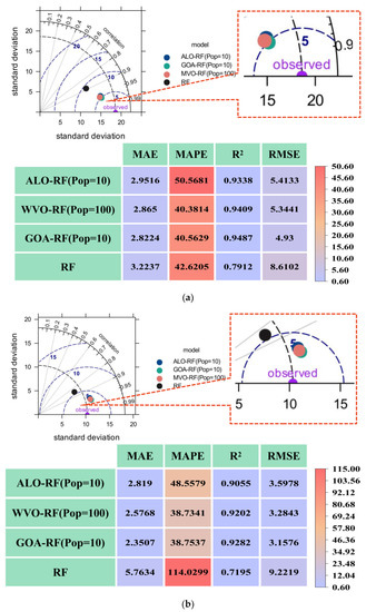
Figure 9.
Comprehensive information on different hybrid model evaluation indicators: (a) Comparative analysis of train set; (b) Comparative analysis of test set.
Figure 7d ranks the evaluation metrics for ALO-RF (Pop = 10), WVO-RF (Pop = 100), GOA-RF (Pop = 10), and RF as shown in Figure 10. The Taylor diagrams in Figure 9 show that the point represented by the GOA-RF model is the closest to the observation point (indicating its smallest RMSE) and its azimuth is the smallest (indicating its largest correlation coefficient), both in the training and testing phases. In conjunction with the comparison and the distribution of Taylor diagrams points shown in Figure 9b, the GOA-RF (Pop = 10) model achieves the optimal GS prediction performance among all hybrid models.
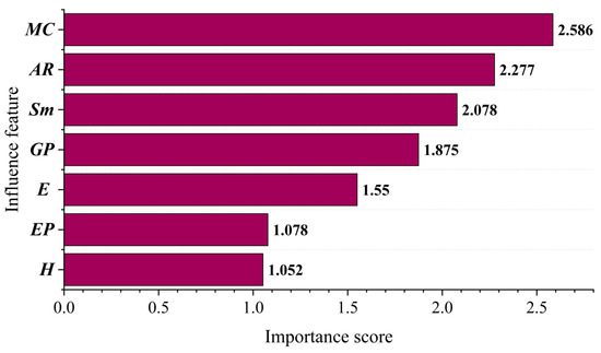
Figure 10.
Importance distribution of each parameter of the optimal model.
Table 5 displays the results of the predictive performance comparison between the proposed GOA-RF model, the unoptimized RF model, and previous studies. The results indicated that the GOA-RF model has significantly improved the GS prediction accuracy compared to previous published results. On the other hand, the GOA algorithm has a significant advantage in optimizing the hyperparameters of RF model for the GS prediction. In addition, there is no significant over- or under-fitting occurred in the GOA-RF (Pop = 10) model using the train and test sets. Therefore, it is recommended to use this model to predict the GS.
Table 5.
Comparison of the prediction effect of GOA-RF (Pop = 10) and previous studies.
4.3. Parameter Importance Analysis
In this study, GOA-RF (Pop = 10) is the best model for the GS prediction. Typically, the out-of-bag (OOB) data error rate is used as the basis for assessing correlation in the RF model, which also represents the contribution degree of variables to the results [96].
Figure 10 illustrates the importance of each relevant parameter for the GS prediction based on the GOA-RF (Pop = 10) model. The results clearly illustrate that MC, AR, Sm, and GP have achieved higher importance scores (2.586, 2.277, 2.078, and 1.875) than E, EP, and H with relatively lower importance scores of 1.55, 1.078, and 1.052, respectively. Therefore, MC, AR, Sm, and GP are more important for the GS prediction than E, EP, and H. Although these seven parameters are different from the GS, the difference in importance scores indicates that neither parameter can be discarded for predicting GS. In future research, additional geological, design, and operational parameters should be considered to improve the model efficiency and precision.
5. Conclusions
In this investigation, three RF models optimized by ALO, WVO, and GOA were developed to predict GS. To avoid data redundancy and improve the scientific rigor of the data, the Pearson correlation analysis was used to exclude feature parameters with strong correlation prior to database construction. The database contains seven input parameters, namely H, AR, EP, Sm, MC, E, and GP.
After completing model construction, the ALO-RF, WVO-RF, and GOA-RF models were evaluated using the evaluation indices MAE, MAPE, R2, and RMSE. The GOA-RF (Pop = 10) model exhibited the best performance in the overall GS prediction, with MAE (Train set: 2.8224; Test set: 2.3507), RMSE (Train set: 4.93; Test set: 3.1576), R2 (Train set: 0.9487; Test set: 0.9282), and MAPE (Train set: 40.5629; Test set: 38.5637). Finally, the importance of each input parameter is calculated using the best prediction model (GOA-RF), and the results indicated that MC, AR, Sm, and GP play a crucial role in the GS prediction.
In future research, more geological, design, and operational parameters should be taken into account to enrich the database and make the prediction of ground settlement more accurate and efficient, therefore providing a more solid scientific foundation for the prevention and control of disasters related to ground settlement. In addition, the proposed GOA-RF model can inspire the development of prediction models in other disciplines.
Author Contributions
Conceptualization, J.Z.; Investigation, P.Y., C.L. and K.P.; Methodology, P.Y. and J.Z.; Project administration, W.W. and J.Z.; Software, P.Y. and C.L.; Supervision, K.P. and J.Z.; Visualization, P.Y., W.Y., W.W. and Y.Q.; Writing—original draft, P.Y.; Writing—review & editing, J.Z., W.W., W.Y., C.L. and Y.Q. All authors have read and agreed to the published version of the manuscript.
Funding
This research is partially supported by the National Natural Science Foundation Project of China (42177164), the Distinguished Youth Science Foundation of Hunan Province of China (2022JJ10073).
Institutional Review Board Statement
Not applicable.
Informed Consent Statement
Not applicable.
Data Availability Statement
The authors do not have permission to share data.
Acknowledgments
This research was funded by the National Science Foundation of China (42177164), and the Distinguished Youth Science Foundation of Hunan Province of China (2022JJ10073).
Conflicts of Interest
The authors declare no conflict of interest.
References
- Skibniewski, M.J. Research trends in information technology applications in construction safety engineering and management. Front. Eng. Manag. 2015, 1, 246–259. [Google Scholar] [CrossRef]
- Zhang, L.; Wu, X.; Liu, H. Strategies to reduce ground settlement from shallow tunnel excavation: A case study in China. J. Constr. Eng. Manag. 2016, 142, 04016001. [Google Scholar] [CrossRef]
- Ou, C.Y.; Teng, F.C.; Wang, I.W. Analysis and design of partial ground improvement in deep excavations. Comput. Geotech. 2008, 35, 576–584. [Google Scholar] [CrossRef]
- Yoo, C.; Lee, D. Deep excavation-induced ground surface movement characteristics—A numerical investigation. Comput. Geotech. 2008, 35, 231–252. [Google Scholar] [CrossRef]
- Dindarloo, S.R.; Siami-Irdemoosa, E. Maximum surface settlement based classification of shallow tunnels in soft ground. Tunn. Undergr. Space Technol. 2015, 49, 320–327. [Google Scholar] [CrossRef]
- Liao, S.M.; Liu, J.H.; Wang, R.L.; Li, Z.M. Shield tunneling and environment protection in Shanghai soft ground. Tunn. Undergr. Space Technol. 2009, 24, 454–465. [Google Scholar] [CrossRef]
- Bjelland, H.; Aven, T. Treatment of uncertainty in risk assessments in the Rogfast road tunnel project. Saf. Sci. 2013, 55, 34–44. [Google Scholar] [CrossRef]
- Papastamos, G.; Stiros, S.; Saltogianni, V.; Kontogianni, V. 3-D strong tilting observed in tall, isolated brick chimneys during the excavation of the Athens Metro. Appl. Geomat. 2015, 7, 115–121. [Google Scholar] [CrossRef]
- Liu, W.; Wu, X.; Zhang, L.; Wang, Y. Probabilistic analysis of tunneling-induced building safety assessment using a hybrid FE-copula model. Struct. Infrastruct. Eng. 2018, 14, 1065–1081. [Google Scholar] [CrossRef]
- O’Reilly, M.P.; New, B.M. Settlements above Tunnels in the United Kingdom—Their Magnitude and Prediction; No. Monograph; Institution of Mining Metallurgy: London, UK, 1982. [Google Scholar]
- Peck, R.B. Deep excavations and tunneling in soft ground. In Proceedings of the 7th International Conference on Soil Mechanics and Foundation Engineering (Mexico), Mexico City, Mexico, 29 August 1969; Volume 1969, pp. 225–290. [Google Scholar]
- Loganathan, N.; Poulos, H.G. Analytical prediction for tunneling-induced ground movements in clays. J. Geotech. Geoenviron. Eng. 1998, 124, 846–856. [Google Scholar] [CrossRef]
- Kasper, T.; Meschke, G. A 3D finite element simulation model for TBM tunnelling in soft ground. Int. J. Numer. Anal. Methods Geomech. 2004, 28, 1441–1460. [Google Scholar] [CrossRef]
- Leca, E.; New, B. Settlements induced by tunneling in soft ground. Tunn. Undergr. Space Technol. 2007, 22, 119–149. [Google Scholar]
- Kim, C.Y.; Bae, G.J.; Hong, S.W.; Park, C.H.; Moon, H.K.; Shin, H.S. Neural network based prediction of ground surface settlements due to tunnelling. Comput. Geotech. 2001, 28, 517–547. [Google Scholar] [CrossRef]
- Ocak, I.; Seker, S.E. Calculation of surface settlements caused by EPBM tunneling using artificial neural network, SVM, and Gaussian processes. Environ. Earth Sci. 2013, 70, 1263–1276. [Google Scholar] [CrossRef]
- Wang, F.; Gou, B.; Qin, Y. Modeling tunneling-induced ground surface settlement development using a wavelet smooth relevance vector machine. Comput. Geotech. 2013, 54, 125–132. [Google Scholar] [CrossRef]
- Zhou, J.; Shi, X.; Du, K.; Qiu, X.; Li, X.; Mitri, H.S. Feasibility of random-forest approach for prediction of ground settlements induced by the construction of a shield-driven tunnel. Int. J. Geomech. 2017, 17, 04016129. [Google Scholar] [CrossRef]
- Zhou, J.; Shi, X.Z.; Du, K.; Qiu, X.Y.; Li, X.B.; Mitri, H.S. Development of the ground movements due to shield tunnelling prediction model using random forests. In Proceedings of the 4th GeoChina International Conference, Shandong, China, 25–27 July 2016; pp. 108–115. [Google Scholar]
- Zhang, P.; Wu, H.N.; Chen, R.P.; Dai, T.; Meng, F.Y.; Wang, H.B. A critical evaluation of machine learning and deep learning in shield-ground interaction prediction. Tunn. Undergr. Space Technol. 2020, 106, 103593. [Google Scholar] [CrossRef]
- Łodygowski, T.; Sumelka, W. Limitations in application of finite element method in acoustic numerical simulation. J. Theor. Appl. Mech. 2006, 44, 849–865. [Google Scholar]
- Attewell, P.B.; Farmer, I.W. Ground deformations resulting from shield tunnelling in London Clay. Can. Geotech. J. 1974, 11, 380–395. [Google Scholar] [CrossRef]
- Yoshikoshi, W.; Watanabe, O.; Takagi, N. Prediction of ground settlements associated with shield tunnelling. Soils Found. 1978, 18, 47–59. [Google Scholar] [CrossRef]
- Hamza, M.; Ata, A.; Roussin, A. Ground movements due to construction of cut and cover structures and slurry shield tunnel of the Cairo metro. Tunn. Undergr. Space Technol. 1999, 14, 281–289. [Google Scholar] [CrossRef]
- Mair, R.J.; Taylor, R.N. Bored tunnelling in the urban environments. In International Society for Soil Mechanics and Foundation Engineering, Proceedings of the Fourteenth International Conference on Soil Mechanics and Foundation Engineering, Hamburg, Germany, 6–12 September 1997; CRC Press: Boca Raton, FL, USA, 1999; Volume 4. [Google Scholar]
- Ercelebi, S.G.; Copur, H.; Ocak, I. Surface settlement predictions for Istanbul Metro tunnels excavated by EPB-TBM. Environ. Earth Sci. 2011, 62, 357–365. [Google Scholar] [CrossRef]
- Chakeri, H.; Ozcelik, Y.; Unver, B. Effects of important factors on surface settlement prediction for metro tunnel excavated by EPB. Tunn. Undergr. Space Technol. 2013, 36, 14–23. [Google Scholar] [CrossRef]
- Sagaseta, C. Analysis of undrained soil deformation due to ground loss. Geotechnique 1987, 37, 301–320. [Google Scholar] [CrossRef]
- Verruijt, A.; Booker, J.R. Surface settlements due to deformation of a tunnel in an elastic half plane. Geotechnique 1998, 48, 709–713. [Google Scholar] [CrossRef]
- Karakus, M.; Fowell, R.J. Effects of different tunnel face advance excavation on the settlement by FEM. Tunn. Undergr. Space Technol. 2003, 18, 513–523. [Google Scholar] [CrossRef]
- Chaudhary, M.T.A. FEM modelling of a large piled raft for settlement control in weak rock. Eng. Struct. 2007, 29, 2901–2907. [Google Scholar] [CrossRef]
- Hisatake, M. A proposed methodology for analysis of ground settlements caused by tunneling, with particular reference to the “buoyancy” effect. Tunn. Undergr. Space Technol. 2011, 26, 130–138. [Google Scholar] [CrossRef]
- Hajjar, M.; Nemati Hayati, A.; Ahmadi, M.M.; Sadrnejad, S.A. Longitudinal settlement profile in shallow tunnels in drained conditions. Int. J. Geomech. 2015, 15, 04014097. [Google Scholar] [CrossRef]
- Lai, J.; Liu, H.; Qiu, J.; Chen, J. Settlement analysis of saturated tailings dam treated by CFG pile composite foundation. Adv. Mater. Sci. Eng. 2016, 2016, 7383762. [Google Scholar] [CrossRef]
- Karakus, M.; Fowell, R.J. Back analysis for tunnelling induced ground movements and stress redistribution. Tunn. Undergr. Space Technol. 2005, 20, 514–524. [Google Scholar] [CrossRef]
- Moeinossadat, S.R.; Ahangari, K. Estimating maximum surface settlement due to EPBM tunneling by Numerical-Intelligent approach—A case study: Tehran subway line 7. Transp. Geotech. 2019, 18, 92–102. [Google Scholar] [CrossRef]
- Lai, H.; Zheng, H.; Chen, R.; Kang, Z.; Liu, Y. Settlement behaviors of existing tunnel caused by obliquely under-crossing shield tunneling in close proximity with small intersection angle. Tunn. Undergr. Space Technol. 2020, 97, 103258. [Google Scholar] [CrossRef]
- Cui, X.; Zhou, R.; Guo, G.; Du, B.; Liu, H. Effects of differential subgrade settlement on slab track deformation based on a DEM-FDM coupled approach. Appl. Sci. 2021, 11, 1384. [Google Scholar] [CrossRef]
- Chen, S.G.; Zhao, J. Modeling of tunnel excavation using a hybrid DEM/BEM method. Comput.-Aided Civ. Infrastruct. Eng. 2002, 17, 381–386. [Google Scholar] [CrossRef]
- Chen, R.P.; Tang, L.J.; Ling, D.S.; Chen, Y.M. Face stability analysis of shallow shield tunnels in dry sandy ground using the discrete element method. Comput. Geotech. 2011, 38, 187–195. [Google Scholar] [CrossRef]
- Bym, T.; Marketos, G.; Burland, J.B.; O’Sullivan, C. Use of a two-dimensional discrete-element line-sink model to gain insight into tunnelling-induced deformations. Géotechnique 2013, 63, 791–795. [Google Scholar] [CrossRef]
- Liu, C.; Pan, L.; Wang, F.; Zhang, Z.; Cui, J.; Liu, H.; Duan, Z.; Ji, X. Three-dimensional discrete element analysis on tunnel face instability in cobbles using ellipsoidal particles. Materials 2019, 12, 3347. [Google Scholar] [CrossRef]
- Gutiérrez-Ch, J.G.; Senent, S.; Zeng, P.; Jimenez, R. DEM simulation of rock creep in tunnels using Rate Process Theory. Comput. Geotech. 2022, 142, 104559. [Google Scholar] [CrossRef]
- Samui, P. Support vector machine applied to settlement of shallow foundations on cohesionless soils. Comput. Geotech. 2008, 35, 419–427. [Google Scholar] [CrossRef]
- Nejad, F.P.; Jaksa, M.B.; Kakhi, M.; McCabe, B.A. Prediction of pile settlement using artificial neural networks based on standard penetration test data. Comput. Geotech. 2009, 36, 1125–1133. [Google Scholar] [CrossRef]
- Le, L.T.; Nguyen, H.; Dou, J.; Zhou, J. A comparative study of PSO-ANN, GA-ANN, ICA-ANN, and ABC-ANN in estimating the heating load of buildings’ energy efficiency for smart city planning. Appl. Sci. 2019, 9, 2630. [Google Scholar] [CrossRef]
- Li, C.; Zhou, J.; Khandelwal, M.; Zhang, X.; Monjezi, M.; Qiu, Y. Six novel hybrid extreme learning machine–swarm intelligence optimization (ELM–SIO) models for predicting backbreak in open-pit blasting. Nat. Resour. Res. 2022, 31, 3017–3039. [Google Scholar] [CrossRef]
- Qiu, Y.; Zhou, J.; Khandelwal, M.; Yang, H.; Yang, P.; Li, C. Performance evaluation of hybrid WOA-XGBoost, GWO-XGBoost and BO-XGBoost models to predict blast-induced ground vibration. Eng. Comput. 2022, 38, 4145–4162. [Google Scholar] [CrossRef]
- Zhou, J.; Dai, Y.; Huang, S.; Armaghani, D.J.; Qiu, Y. Proposing several hybrid SSA—Machine learning techniques for estimating rock cuttability by conical pick with relieved cutting modes. Acta Geotech. 2022, 1–16. [Google Scholar] [CrossRef]
- Zhou, J.; Dai, Y.; Du, K.; Khandelwal, M.; Li, C.; Qiu, Y. COSMA-RF: New intelligent model based on chaos optimized slime mould algorithm and random forest for estimating the peak cutting force of conical picks. Transp. Geotech. 2022, 36, 100806. [Google Scholar] [CrossRef]
- Zhou, J.; Huang, S.; Tao, M.; Khandelwal, M.; Dai, Y.; Zhao, M. Stability prediction of underground entry-type excavations based on particle swarm optimization and gradient boosting decision tree. Undergr. Space 2023, 9, 234–249. [Google Scholar] [CrossRef]
- Shi, J.; Ortigao, J.A.R.; Bai, J. Modular neural networks for predicting settlements during tunneling. J. Geotech. Geoenviron. Eng. 1998, 124, 389–395. [Google Scholar] [CrossRef]
- Suwansawat, S.; Einstein, H.H. Artificial neural networks for predicting the maximum surface settlement caused by EPB shield tunneling. Tunn. Undergr. Space Technol. 2006, 21, 133–150. [Google Scholar] [CrossRef]
- Goh, A.T.; Hefney, A.M. Reliability assessment of EPB tunnel-related settlement. Geomech. Eng. 2010, 2, 57–69. [Google Scholar] [CrossRef]
- Boubou, R.; Emeriault, F.; Kastner, R. Artificial neural network application for the prediction of ground surface movements induced by shield tunnelling. Can. Geotech. J. 2010, 47, 1214–1233. [Google Scholar] [CrossRef]
- Marto, A.; Hajihassani, M.; Kalatehjari, R.; Namazi, E.; Sohaei, H. Simulation of longitudinal surface settlement due to tunnelling using artificial neural network. Int. Rev. Model. Simul. 2012, 5, 1024–1031. [Google Scholar]
- Pourtaghi, A.; Lotfollahi-Yaghin, M.A. Wavenet ability assessment in comparison to ANN for predicting the maximum surface settlement caused by tunneling. Tunn. Undergr. Space Technol. 2012, 28, 257–271. [Google Scholar] [CrossRef]
- Hasanipanah, M.; Noorian-Bidgoli, M.; Jahed Armaghani, D.; Khamesi, H. Feasibility of PSO-ANN model for predicting surface settlement caused by tunneling. Eng. Comput. 2016, 32, 705–715. [Google Scholar] [CrossRef]
- Zhang, L.; Wu, X.; Ji, W.; AbouRizk, S.M. Intelligent approach to estimation of tunnel-induced ground settlement using wavelet packet and support vector machines. J. Comput. Civ. Eng. 2017, 31, 04016053. [Google Scholar] [CrossRef]
- Kohestani, V.R.; Bazarganlari, M.R.; Asgari Marnani, J. Prediction of maximum surface settlement caused by earth pressure balance shield tunneling using random forest. J. AI Data Min. 2017, 5, 127–135. [Google Scholar]
- Goh, A.T.C.; Zhang, W.; Zhang, Y.; Xiao, Y.; Xiang, Y. Determination of earth pressure balance tunnel-related maximum surface settlement: A multivariate adaptive regression splines approach. Bull. Eng. Geol. Environ. 2018, 77, 489–500. [Google Scholar] [CrossRef]
- Shi, S.; Zhao, R.; Li, S.; Xie, X.; Li, L.; Zhou, Z.; Liu, H. Intelligent prediction of surrounding rock deformation of shallow buried highway tunnel and its engineering application. Tunn. Undergr. Space Technol. 2019, 90, 1–11. [Google Scholar] [CrossRef]
- Chen, R.P.; Zhang, P.; Kang, X.; Zhong, Z.Q.; Liu, Y.; Wu, H.N. Prediction of maximum surface settlement caused by earth pressure balance (EPB) shield tunneling with ANN methods. Soils Found. 2019, 59, 284–295. [Google Scholar] [CrossRef]
- Chen, R.; Zhang, P.; Wu, H.; Wang, Z.; Zhong, Z. Prediction of shield tunneling-induced ground settlement using machine learning techniques. Front. Struct. Civ. Eng. 2019, 13, 1363–1378. [Google Scholar] [CrossRef]
- Zhang, K.; Lyu, H.M.; Shen, S.L.; Zhou, A.; Yin, Z.Y. Evolutionary hybrid neural network approach to predict shield tunneling-induced ground settlements. Tunn. Undergr. Space Technol. 2020, 106, 103594. [Google Scholar] [CrossRef]
- Zhang, P.; Wu, H.N.; Chen, R.P.; Chan, T.H. Hybrid meta-heuristic and machine learning algorithms for tunneling-induced settlement prediction: A comparative study. Tunn. Undergr. Space Technol. 2020, 99, 103383. [Google Scholar] [CrossRef]
- Liu, X.; Hussein, S.H.; Ghazali, K.H.; Tung, T.M.; Yaseen, Z.M. Optimized adaptive neuro-fuzzy inference system using metaheuristic algorithms: Application of shield tunnelling ground surface settlement prediction. Complexity 2021, 2021, 6666699. [Google Scholar] [CrossRef]
- Zhang, W.G.; Li, H.R.; Wu, C.Z.; Li, Y.Q.; Liu, Z.Q.; Liu, H.L. Soft computing approach for prediction of surface settlement induced by earth pressure balance shield tunneling. Undergr. Space 2021, 6, 353–363. [Google Scholar] [CrossRef]
- Breiman, L. Random forests. Mach. Learn. 2001, 45, 5–32. [Google Scholar] [CrossRef]
- Chen, Y.; Yong, W.; Li, C.; Zhou, J. Predicting the Thickness of an Excavation Damaged Zone around the Roadway Using the DA-RF Hybrid Model. Comput. Model. Eng. Sci. 2022, 1–20. [Google Scholar] [CrossRef]
- Dai, Y.; Khandelwal, M.; Qiu, Y.; Zhou, J.; Monjezi, M.; Yang, P. A hybrid metaheuristic approach using random forest and particle swarm optimization to study and evaluate backbreak in open-pit blasting. Neural Comput. Appl. 2022, 34, 6273–6288. [Google Scholar] [CrossRef]
- Han, H.; Jahed Armaghani, D.; Tarinejad, R.; Zhou, J.; Tahir, M.M. Random forest and bayesian network techniques for probabilistic prediction of flyrock induced by blasting in quarry sites. Nat. Resour. Res. 2020, 29, 655–667. [Google Scholar] [CrossRef]
- Li, C.; Zhou, J.; Tao, M.; Du, K.; Wang, S.; Armaghani, D.J.; Mohamad, E.T. Developing hybrid ELM-ALO, ELM-LSO and ELM-SOA models for predicting advance rate of TBM. Transp. Geotech. 2022, 36, 100819. [Google Scholar] [CrossRef]
- Yu, Z.; Shi, X.; Zhou, J.; Chen, X.; Qiu, X. Effective assessment of blast-induced ground vibration using an optimized random forest model based on a Harris hawks optimization algorithm. Appl. Sci. 2020, 10, 1403. [Google Scholar] [CrossRef]
- Zhang, H.; Zhou, J.; Jahed Armaghani, D.; Tahir, M.M.; Pham, B.T.; Huynh, V.V. A combination of feature selection and random forest techniques to solve a problem related to blast-induced ground vibration. Appl. Sci. 2020, 10, 869. [Google Scholar] [CrossRef]
- Zhou, J.; Li, E.; Wei, H.; Li, C.; Qiao, Q.; Armaghani, D.J. Random forests and cubist algorithms for predicting shear strengths of rockfill materials. Appl. Sci. 2019, 9, 1621. [Google Scholar] [CrossRef]
- Zhou, J.; Asteris, P.G.; Armaghani, D.J.; Pham, B.T. Prediction of ground vibration induced by blasting operations through the use of the Bayesian Network and random forest models. Soil Dyn. Earthq. Eng. 2020, 139, 106390. [Google Scholar] [CrossRef]
- Zhou, J.; Chen, Y.; Yong, W. Performance evaluation of hybrid YYPO-RF, BWOA-RF and SMA-RF models to predict plastic zones around underground powerhouse caverns. Geomech. Geophys. Geo-Energy Geo-Resour. 2022, 8, 179. [Google Scholar] [CrossRef]
- Zhou, J.; Huang, S.; Qiu, Y. Optimization of random forest through the use of MVO, GWO and MFO in evaluating the stability of underground entry-type excavations. Tunn. Undergr. Space Technol. 2022, 124, 104494. [Google Scholar] [CrossRef]
- Dong, L.J.; Li, X.B.; Kang, P.E.N.G. Prediction of rockburst classification using Random Forest. Trans. Nonferrous Met. Soc. China 2013, 23, 472–477. [Google Scholar] [CrossRef]
- Tao, H.; Jingcheng, W.; Langwen, Z. Prediction of hard rock TBM penetration rate using random forests. In Proceedings of the 27th Chinese Control and Decision Conference (2015 CCDC), Qingdao, China, 23–25 May 2015; IEEE: New York, NY, USA; pp. 3716–3720. [Google Scholar]
- Liu, L.; Zhou, W.; Gutierrez, M. Effectiveness of predicting tunneling-induced ground settlements using machine learning methods with small datasets. J. Rock Mech. Geotech. Eng. 2022, 14, 1028–1041. [Google Scholar] [CrossRef]
- Mirjalili, S. The ant lion optimizer. Adv. Eng. Softw. 2015, 83, 80–98. [Google Scholar] [CrossRef]
- Mirjalili, S.; Mirjalili, S.M.; Hatamlou, A. Multi-verse optimizer: A nature-inspired algorithm for global optimization. Neural Comput. Appl. 2016, 27, 495–513. [Google Scholar] [CrossRef]
- Steinhardt, P.J.; Turok, N. The cyclic model simplified. N. Astron. Rev. 2005, 49, 43–57. [Google Scholar] [CrossRef]
- Saremi, S.; Mirjalili, S.; Lewis, A. Grasshopper optimisation algorithm: Theory and application. Adv. Eng. Softw. 2017, 105, 30–47. [Google Scholar] [CrossRef]
- Hulme, T.W.; Burchell, A.J. Tunnelling projects in Singapore: An overview. Tunn. Undergr. Space Technol. 1999, 14, 409–418. [Google Scholar] [CrossRef]
- Izumi, C.; Khatri, N.N.; Norrish, A.; Davies, R. Stability and Settlement Due to Bored Tunnelling for LTA, NEL. In Tunnels and Underground Structures; Routledge: London, UK, 2017; pp. 555–560. [Google Scholar]
- Shirlaw, J.N.; Ong, J.C.W.; Rosser, H.B.; Tan, C.G.; Osborne, N.H.; Heslop, P.E. Local settlements and sinkholes due to EPB tunnelling. Proc. Inst. Civ. Eng.-Geotech. Eng. 2003, 156, 193–211. [Google Scholar] [CrossRef]
- Sharma, J.S.; Chu, J.; Zhao, J. Geological and geotechnical features of Singapore: An overview. Tunn. Undergr. Space Technol. 1999, 14, 419–431. [Google Scholar] [CrossRef]
- Li, E.; Yang, F.; Ren, M.; Zhang, X.; Zhou, J.; Khandelwal, M. Prediction of blasting mean fragment size using support vector regression combined with five optimization algorithms. J. Rock Mech. Geotech. Eng. 2021, 13, 1380–1397. [Google Scholar] [CrossRef]
- Zhou, J.; Qiu, Y.; Armaghani, D.J.; Zhang, W.; Li, C.; Zhu, S.; Tarinejad, R. Predicting TBM penetration rate in hard rock condition: A comparative study among six XGB-based metaheuristic techniques. Geosci. Front. 2021, 12, 101091. [Google Scholar] [CrossRef]
- Zhou, J.; Li, X.; Mitri, H.S. Comparative performance of six supervised learning methods for the development of models of hard rock pillar stability prediction. Nat. Hazards 2015, 79, 291–316. [Google Scholar] [CrossRef]
- Zhou, J.; Li, X.; Mitri, H.S. Classification of rockburst in underground projects: Comparison of ten supervised learning methods. J. Comput. Civ. Eng. 2016, 30, 04016003. [Google Scholar] [CrossRef]
- Taylor, K.E. Summarizing multiple aspects of model performance in a single diagram. J. Geophys. Res. Atmos. 2001, 106, 7183–7192. [Google Scholar] [CrossRef]
- Adusumilli, S.; Bhatt, D.; Wang, H.; Bhattacharya, P.; Devabhaktuni, V. A low-cost INS/GPS integration methodology based on random forest regression. Expert Syst. Appl. 2013, 40, 4653–4659. [Google Scholar] [CrossRef]


Disclaimer/Publisher’s Note: The statements, opinions and data contained in all publications are solely those of the individual author(s) and contributor(s) and not of MDPI and/or the editor(s). MDPI and/or the editor(s) disclaim responsibility for any injury to people or property resulting from any ideas, methods, instructions or products referred to in the content. |
© 2023 by the authors. Licensee MDPI, Basel, Switzerland. This article is an open access article distributed under the terms and conditions of the Creative Commons Attribution (CC BY) license (https://creativecommons.org/licenses/by/4.0/).