Article

Study on the Localization of Defects in Typical Steel Butt Welds Considering the Effect of Residual Stress

1
School of Civil Engineering, Chongqing Jiaotong University, Chongqing 400074, China
2
State Key Laboratory of Moutain Bridge and Tunnel Engineering, Chongqing Jiaotong University, Chongqing 400074, China
*
Author to whom correspondence should be addressed.
Appl. Sci. 2023, 13(4), 2648; https://doi.org/10.3390/app13042648
Submission received: 20 January 2023 / Revised: 12 February 2023 / Accepted: 15 February 2023 / Published: 18 February 2023

Abstract

:
When using magnetic memory detection technology to locate weld cracks and porous defects, the traditional zero-point polarity theory leads to misjudgments in defect location and difficulty in distinguishing between the residual stress and the magnetic signals generated by defects due to the influence of external noise and residual stress. Therefore, this paper considers the different mechanisms of magnetic signal generation in areas where crack- and porosity-type defects and residual stresses are located and discusses research focused on the detection of weld defect localization considering the influence of residual stresses. Using the mechanism of magnetic signal generation as a starting point, the three-dimensional magnetic modulus gradient polarity determination method is proposed to distinguish residual stress and defects’ magnetic signals. Through the COMSOL simulation of a welding defect’s finite element magnetic signal, the resulting magnetic signal is converted into a characteristic determination formula for characterization. To verify the accuracy of the simulated characterization, the 3D magnetic signal is extracted and verified manually. Finally, a double orthogonal wavelet transform is introduced to eliminate the random noise in the gradient of the three-dimensional magnetic modulus. The results show that the theoretical analysis, numerical simulation, and experimental results agree with each other. The three-dimensional magnetic modulus gradient values of cracks and pores are much higher than that of the defect-free residual stress area. The three-dimensional magnetic gradient modulus can locate defects and characterize the lengths of defects. The dual orthogonal wavelet eliminates noise interference while improving the accuracy of locating three-dimensional magnetic modulus gradient defects.

1. Introduction

Steel is widely used among welded structures due to characteristics such as uniformity of material and simplicity of manufacture; welding is an important connection method for structures widely used in modern industry [1]. The presence of cracks and other welding defects in welded joints seriously affects the safety performance of welded structures and makes the welded area hazardous [2,3]. Presently, the main methods of non-destructive testing are magnetic particle, eddy current, ultrasonic, and ray methods, as well as other testing methods, which play an essential role in ensuring the safety and reliability of equipment and preventing unexpected accidents [4,5,6]. Among NDT (non-destructive testing) methods, the magnetic memory inspection method can detect both surface and internal defects and has the advantages of high sensitivity, fast detection, low surface cleanliness, low cost, and simple operation compared with other NDT methods; thus, the magnetic memory method has attracted the attention of many scholars [7].
The goal of magnetic memory detection technology is to extract the magnetic field leakage on the surface of the specimen to locate the defect. Before locating the defect in the specimen, the magnetic memory signal characteristics that characterize the defect should be extracted so that the location information of the defect can be accurately determined [8].
The literature [9,10,11] investigates the effects of weld orientation and phase change on the distribution of residual stresses in welds using finite elements, laying the foundation for utilizing magnetic memory detection within welding simulations. Maciej Roskosz [12] proposed that the metal magnetic memory detection method is effective for the detection of welding defects in in-service equipment. Currently, as a defect signal characteristic, Doubov [13] proposed the normal component of the magnetic memory signal over zero-point polarity theory, and the tangential component has extreme values as criteria for determining defects. However, this feature has been controversial since its introduction. Researchers have found, through a large number of experiments, that the tangential and normal characteristics of the judgment are not reliable. By comparing the results of online and offline testing, Dawei Yin et al. [14] concluded that specimens are influenced by the ambient magnetic fields during online inspections, and the over-zero-point feature does not accurately reflect the stress concentrations and defect sites. Dong Lihong et al. [15] found, through static tensile loading experiments, that the position of the over-zero point is not fixed when the member is subjected to changes in the magnitude of the load action, and there is a gradual drift of the over-zero point’s position toward the final fracture position as the stress increases. Qingmin Gao et al. [16] studied the relationship between the tangential and normal signals of magnetic memory and the detection direction and extraction path using finite element simulation, and the normal and tangential components of the leakage field showed large undulations away from the region of stress concentration. Ma Hu et al. [17] studied the effect of residual stress and cracks in welds on the magnetic memory signal and found that the presence of residual stress in welds makes the magnetic signal distribution intertwined with crack defects’ signal distribution, which seriously affects the tangential and normal characteristics’ discriminative features. It can be seen that the tangential and normal signal characteristics of the magnetic field signal are easily affected by additional factors. In contrast, the magnetic field is distributed in a spatial state, so characterization with a single directional signal affected by many influencing factors is ,inevitably,misjudged. Thus, it is also impossible to accurately extract information about the defect site; Chen, Hailong, et al. [18,19] used the magnetic gradient tensor method to extract the fine signal of the nine-dimensional component of the magnetic signal of a magnetic field. The influence of magnetic memory detection direction on the detection signal was eliminated by scaling, so the multidimensional magnetic memory signal was showed to have an important role in accurately positioning defects [20]. Since the magnetic memory signal is a weak magnetic field signal, the measured magnetic signal in the actual inspection is affected by the roughness of the test piece’s surface, the ambient background magnetic field, and the system noise, which results in the magnetic signal containing a large amount of interference noise [21,22]. Since wavelet transform has the characteristics of a “mathematical microscope” and has multi-resolution, research [23,24] has found that it has more applications in magnetic memory signal processing, and the interference of random noise in magnetic memory signals can be eliminated by using wavelet noise.
In this paper, with the help of magnetic charge theory and electromagnetism theory, theoretical support for the difference in magnetic permeability in the two regions is unearthed by using the phenomenon wherein the number of magnetic charges gathered in pores and cracks far exceeds that in the region where the residual stress is located. Additionally, considering that information on the defect site cannot be accurately extracted from a single directional signal, three-dimensional magnetic modulus gradient extremes [25,26] are proposed to characterize air-type defects among the welds. Finally, the feasibility and validity of the method are demonstrated with the help of simulations and experimental validation based on the elimination of the effect of random interference noise on the 3D magnetic modulus gradient polarity. This study is the first to complete a coupled thermal force–magnetic analysis, and provides a reference for finite element simulation studies focused on magnetic memory. The proposed determination characteristics accurately locate welding defects and provide a good judgment for defect detection in practical engineering.

2. Theoretical Analysis

A large amount of positive and negative magnetic charge gathers around defects and residual stress boundaries. From the theory of electromagnetism, for a magnetic dipole with magnetic moment m, the magnetic field generated at r is [27]
H = m r 3   ( 2 e r cos θ + e θ sin θ )
where e r and e θ are the basis vectors of the vector diameter r and the polar angle θ in spherical coordinates, respectively. According to the vector operation rule, the absolute value of the combined vector is the sum of the squares of the basis vectors. Therefore, the absolute value of H is
H = m r 3 ( 1 + 3 cos 2 θ ) 1 2
Since the defect is buried inside the specimen and the magnetic signal of the residual stress is scattered outward from inside the weld, the distance of the defect and the residual stress-affected zone from the specified signal location is set to R, the adequate thickness of the defect and the residual stress-affected zone is dR, and the number of magnetic charge particles carried within the adequate thickness is dn; therefore, the mean value of the magnetic field generated on the detection probe is [28]
H R 2 ¯ = d n h 2 ¯ = d n m 2 R 6 0 π 2 ( 1 + 3 cos 2 θ ) sin θ d θ = 2 d n m 2 R 6
If the number of particles per unit volume in the aggregate is n0, then dn = n04 π R2dR, so the above equation can be rewritten as
H R 2 ¯ = 8 π n 0 m 2 d R R 4
Equation (4) is integrated over the entire volume, and the mean square value of the magnetic field generated by all particles in the ensemble at the specified point, excluding the specified point, is obtained, i.e., [29]
H m 2 ¯ = 8 π n 0 m 2 r 0 d R R 4 = 8 π n 0 m 2 3 r 0 3
The lower limit of the integral of Equation (5) is taken as r0 because the specified point of a particle occupies a linear degree of r0, that is, a particle occupies a space of r03. As there are n0 particles in the unit volume of the aggregate, n0 r03 = 1, so
H m 2 ¯ = 8 π n 0 2 m 2 3 n 0 r 0 3 = 8 π 3 n 0 2 m 2
where
H m 2 ¯ = H x 2 ¯ + H y 2 ¯ + H z 2 ¯
Residual stresses and weld defects of different sizes occur during the reworking of welded seams. After welding, a large amount of magnetic charge is gathered in the residual stress area and the defect area, forming N and S poles, causing the residual stress area and the defect area to scatter the magnetic field outward. From Equations (6) and (7), it is known that the magnetic field strength is related to the number of magnetic charges per unit volume, n0. According to the principle of minimum magnetic free energy of the magnetic charge system, under the action of Coulomb force, a large amount of magnetic charge of the ferromagnetic component gathers at the boundary of the defect, making the number of magnetic charges n0 per unit volume surge. In the residual stress region, due to the continuous distribution of the ferromagnetic medium, the magnetic charge distribution is sparse and uniform, making the magnetic charge number per unit volume n0 much less than that in the defect region, which leads to a sudden increase in the magnetic field strength in the defect region.
In contrast, the magnetic field strength in the residual stress region is lower than that in the defect region. Therefore, the differential value of the magnetic field strength has a very high amplitude at the defect due to a large amount of magnetic charge aggregation. At the same time, extreme values also appear at the residual stress region, but the amplitude of the residual stress is much lower than that of the defect area because the magnetic charge is much less aggregated compared to that of the defect area. This leads us to propose a new characteristic expression: three-dimensional magnetic modulus gradient extrema, to reflect the defect location and to distinguish between defects and residual stresses, whose formulation is shown in Equation (8):
D = | d H x 2 ¯ + H y 2 ¯ + H z 2 ¯ d x | max
where dx is the differential value of the magnetic signal along the weld direction under the influence of defects and residual stress.

3. Simulation Analysis of Thermal Force–Magnetic Coupling under a Three-Dimensional Geomagnetic Field

Due to the complex stress distribution in butt welds after welding, it was difficult to perform direct thermal force–magnetic coupling simulation. Therefore, COMSOL software was used to simulate the welding process, and indirect coupling was used to solve the distribution law of the surface leakage field of the butt weld and its near-air layer under the combined effect of residual stress and the geomagnetic field.

3.1. Force–Magnetic Coupling Relationship

The force–magnetic coupling model for ferromagnetic materials in a three-dimensional geomagnetic field [30] is as follows:
μ = μ T ( 1 + b H μ T ) ( a 0 + a 1 | σ | m · e n | σ | )
where μ is the magnetic permeability after application of stress; μ T denotes no initial magnetic permeability 285; b represents constants related to the properties of the material itself 2.5; and H is the magnitude of the geomagnetic field (39.8 A/m). When σ < 50 MPa, a 0 = 0.76804; a 1 = 0.000916; m = 1.90412; and n = −0.03353. When σ ≥ 50 MPa, a 0 = −0.00447; a 1 = 0.04108; m = 1.55499; and n = −0.03148.

3.2. Force–Magnetic Coupling Finite Element Simulation

In this paper, COMSOL is used for coupled thermal force–magnetic finite element simulation, modeled according to the actual dimensions of the specimen. The size of the flat-plate butt specimen is 400 mm × 385 mm × 10 mm, the width of the welding channel is 13 mm, and the V-shaped weld crack- and porosity-type defects with length 2 mm, width 1 mm, and depth 2 mm are established at the center of the weld seam. After the model is established to divide the mesh, because it involves the study of weld cracks and porosity defects in modelling the mesh refinement at the weld, away from the weld, calculation accuracy requirements are not high, and sparse mesh is used to establish the finite element mesh, as shown in Figure 1 below. This model uses detailed tetrahedral cells at the weld seam and equidistant hexahedral cells away from the weld seam, with a total of 43,480 cells and 24,293 mesh vertices. The magnetic field, solid heat transfer, and solid mechanics modules are selected for multi-physics field coupling analysis.

3.3. Simulation Results of Force–Magnetic Coupling

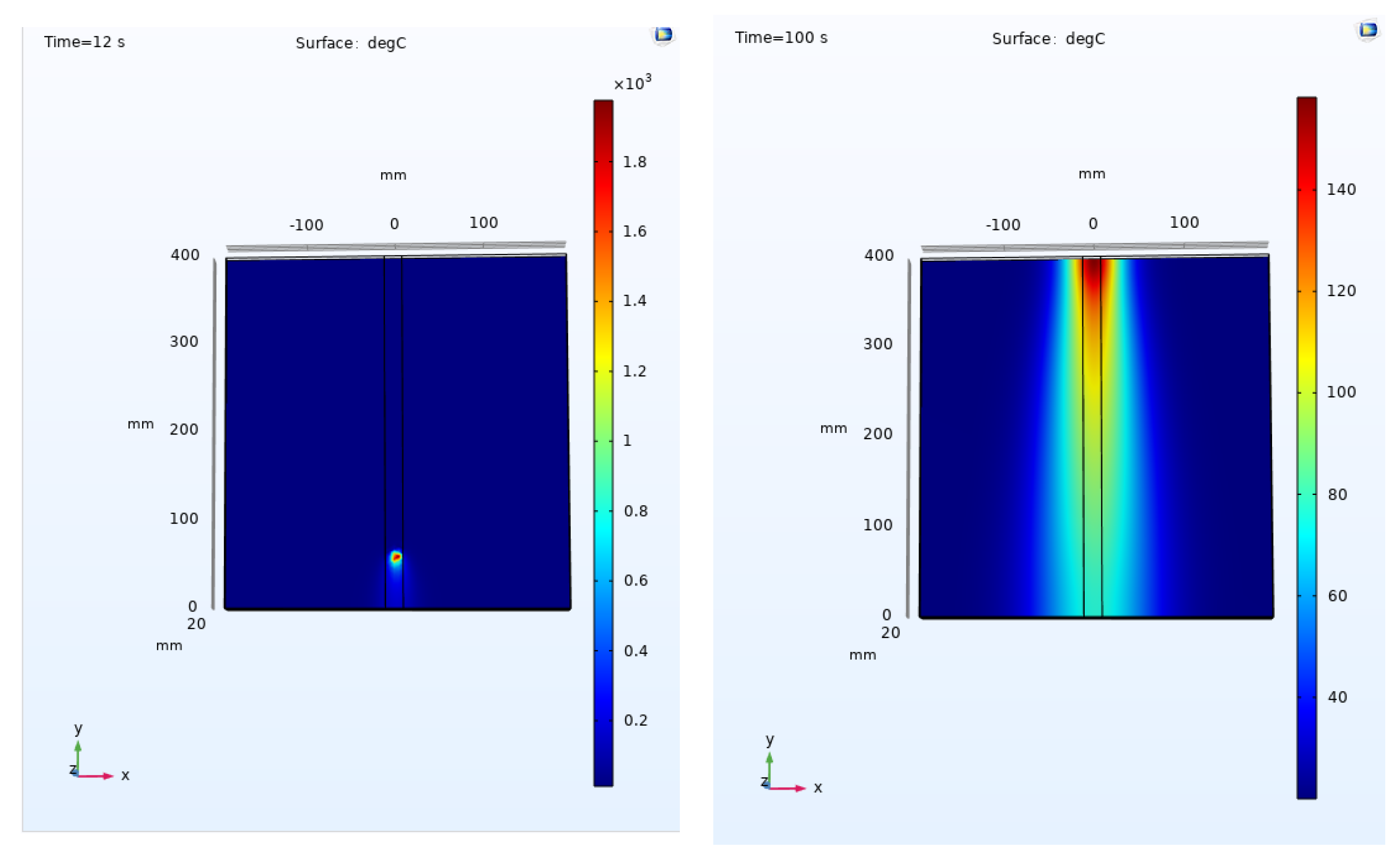
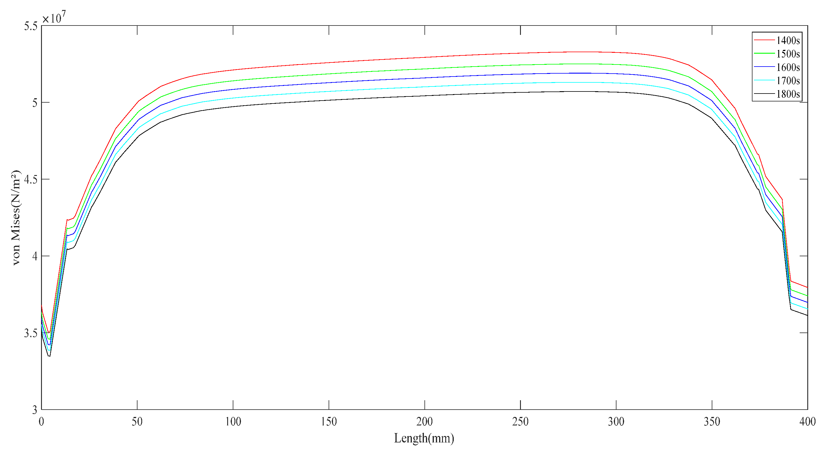
Welding Residual Stress Simulation

The welding process in COMSOL is a transient heat transfer process, which is manifested in two main aspects of heat transfer: heat transfer from the center of the weld to the edge of the specimen on the one hand, and heat radiation from the specimen to the air on the other. The heat transfer coefficient between the specimen and the outside world was set to 110 W/(m2·°C), and the ambient temperature was set to 20 °C. The heat source for welding was applied using a Gaussian mobile heat source, simulated as shown in Figure 2. The heating radius of the welding is 5 mm, the welding probe moves at a speed of 5 mm/s, the distributed power q of the Gaussian heat source is 8 × 10⁷ [W/m2], and the boundary heat source is on the upper surface of the flat welded specimen. The convection heat dissipation coefficient of the heat flux is 5 w/(m2·k), and the coefficient of thermal expansion is 12.2 × 10⁻⁶. Figure 2 shows the applied Gaussian heat source and the diffusion of the temperature field.
The whole welding process, in the 80 s from the beginning of welding to the cooling of the steel plate after 1400 s, is closest to the actual welding state. Five different periods of heat dissipation of the weld area and their equivalent force distributions are shown in Figure 3, namely 1400 s, 1500 s, 1600 s, 1700 s, and 1800 s. As can be seen from the figure, the trend of the distribution of the equivalent force for each period is the same. The peak is reached at around the 50 mm region and then enters a stable state. When reaching the 350 mm region, the equivalent force decreases sharply. It is noteworthy that the equivalent force is the largest after 1400 s of heat dissipation. Therefore, the state after 1400 s of heat dissipation was chosen for subsequent magnetic signal characterization.

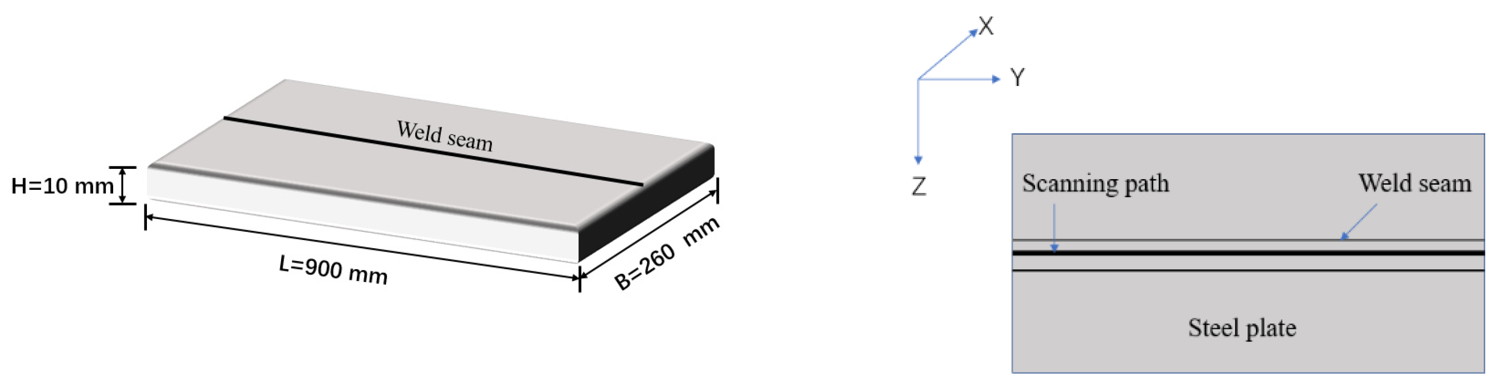
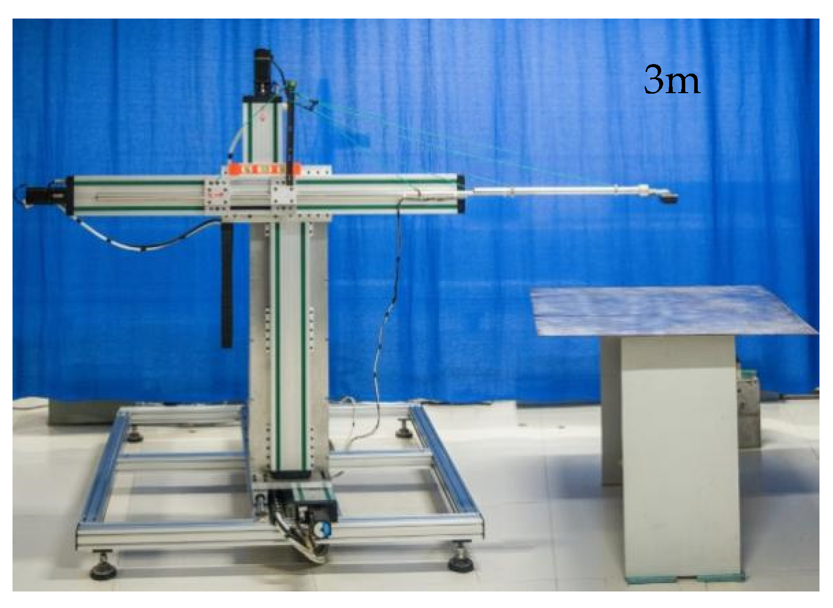
4. Experimental Design

Regarding the production of welded test block A, the base material was Q235 steel, the test block had a width of 260 mm and a length of 900 mm, the thickness of the test piece was 10 mm, and the width of the weld was 13 mm, as shown in Figure 4.
To ensure that the test process was not disturbed by the external environment and to exclude the influence of the surrounding magnetic field, the workpiece was placed in a stable place, and no strong magnetic sources were in proximity. Moisture and grease generated by hydrogen, nitrogen, carbon monoxide, water vapor, and other reactive gases that are not fused to the metal can produce porosity in the weld; high detention, high thermal stress, high welding current, and excessive welding speed can produce welding cracks. The manual arc welding method was used to produce defects inside the same weld, followed by an ultrasound to verify the number of defects, the location, and the burial depth, as shown in Figure 5; ultrasound detections can be seen at points 125 mm, 320 mm, and 530 mm in the weld, denoting three crack- and porosity-type defects.
The detection instrument used in this thesis was a three-axis magnetic intensity detection system with a HMR2300 magnetometer as the core (shown in Figure 6). The detection device had three magnetoresistive sensors distributed in the X, Y, and Z directions, which can measure the three-dimensional magnetic field strength in space with high accuracy.

5. Results and Discussion

5.1. Magnetic Signal Distribution Pattern under the Influence of Residual Stress

The AC/DC magnetic field analysis module is imported into COMSOL and the magnetization of the welded component is carried out. The stress permeability of the component is analyzed using Equation (9), after which the magnetic signals of the component in the X, Y, and Z directions are derived under the influence of the equivalent residual stress after 1400 s of heat dissipation, as shown in Figure 7a–c.
From Figure 4d, it can be seen that the equivalent stress in the weld after 1400 s of heat dissipation starts to rise abruptly from the starting point and then shows a decreasing trend around the 10 mm region, after which it starts to rise sharply. In the 50 mm region, the stress reaches 51 MPa, after which the equivalent stress rises slowly with the length of the weld and then decreases sharply after rising to 56 MPa in the 350 mm region. As can be seen in Figure 7a–c, the Z-direction normal component produces an abrupt change in the region of 10–55 mm and then a sharp, abrupt change after 350 mm, but no zero-point phenomenon occurs, while a high-amplitude zero-point phenomenon occurs at the crack- and porosity-type defects at 200 mm, which is due to the significant irregular accumulation of magnetic charge in the crack- and porosity-type defect region, where the magnetic permeability of the defect site is air-type magnetic permeability; thus, the magnetic permeability changes abruptly, resulting in the zero-point phenomenon. The three components in the region of 10–50 mm and the region beyond 350 mm are consistent with each other in the range of the abrupt change in the equivalent effect force, in which the tangential Y component produces a high-amplitude jitter, and its extreme value affects the judgment of the defects to some extent. After that, the three-dimensional magnetic modulus gradient signal is extracted as shown in Figure 4e, and its extreme value exactly corresponds to the center of the defect, and the extreme value of the residual stress-affected region (Figure 7e., in the 10–50 mm region and the region beyond 350 mm) is much lower than the extreme value of the defect region.
In order to further explore the influence of residual stress on the magnetic signal, a defect of the same size is preset at 50 mm. The magnetic signal components in X, Y, and Z directions after 1400 s of heat dissipation are shown in Figure 8a–c. The traditional discriminative way is no longer obvious and fails to accurately locate the defect. We invert the 3D magnetic modulus gradient and, in Figure 8e, it can be seen that the 3D magnetic modulus gradient accurately locates the defect at 50 mm.
The existing theory suggests that the magnetic memory technique can detect defects below the millimeter level. However, it is unknown whether defects below the millimeter level can be detected under residual stress. For this reason, in this paper, the defect size is changed to 0.5 mm long by 0.5 mm wide by 0.5 mm deep and placed at 50 mm, and the magnetic signal after 1400 s heat of dissipation is studied to obtain the three-dimensional magnetic modulus gradient diagram as shown in Figure 9. It can be seen that the extreme value of the three-dimensional magnetic modulus gradient corresponds to 51.33 mm, which is 1.08 mm away from the initially intended location, so the magnetic memory detection technique cannot accurately detect the location of defects below the millimeter level under the influence of residual stress.

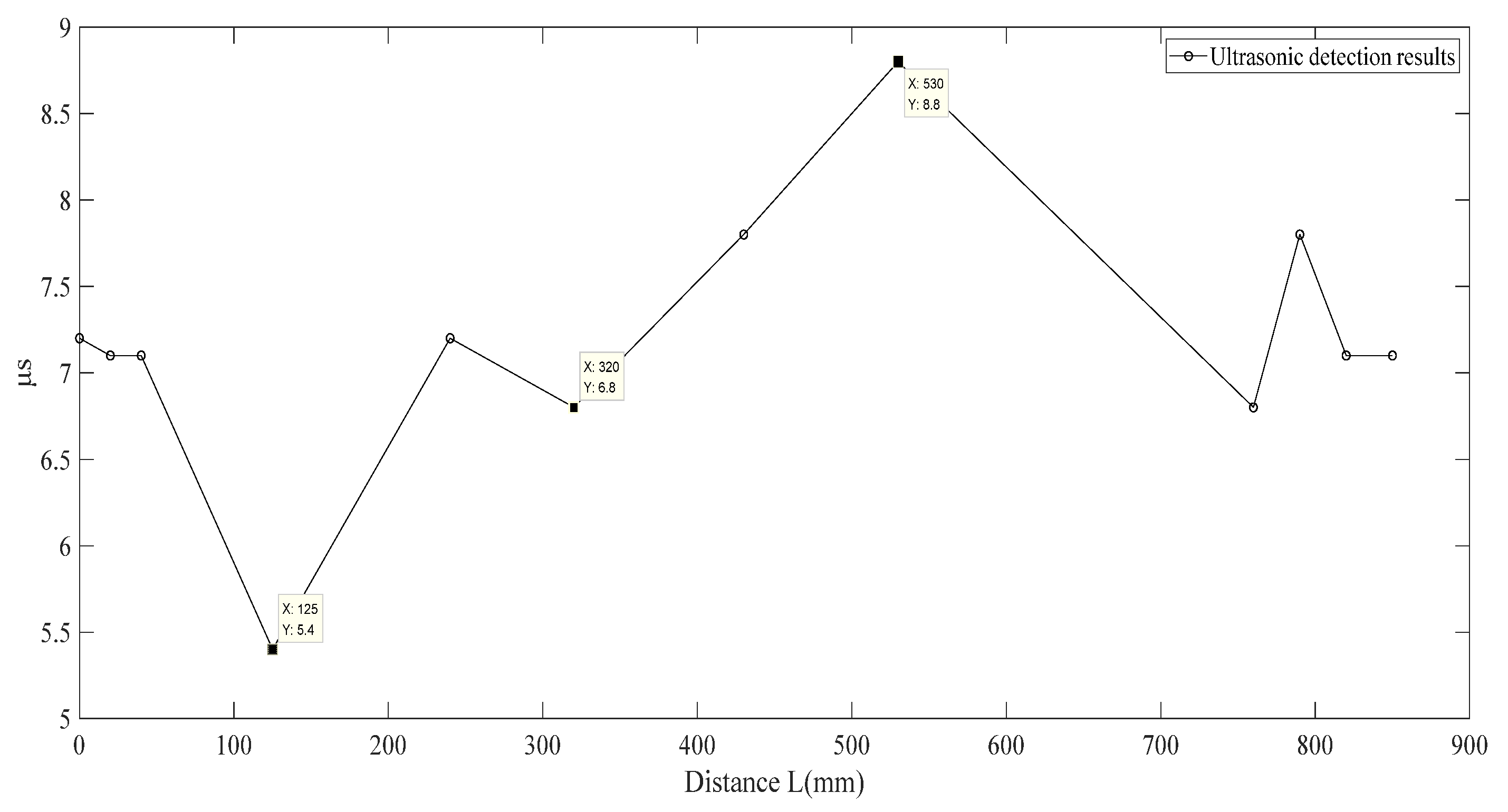
5.2. Quantitative Analysis of Welding Defect Detection

In general, the quantitative factors describing welding defects are the length of the defect, the angle, and the depth of burial of the defect, but in actual engineering, the length of the defect receives more attention. Therefore, the length of the defect is selected as the characteristic quantity for the quantitative study of welding defects.
Defect length was the independent variable. We used the condition of 1400 s of heat dissipation under the effect of residual stress as a simulation of the working conditions, set different length values (size are 1 mm, 2 mm, 3 mm, 4 mm, 5 mm, 6 mm, and 7 mm) for crack- and porosity-type defects in the welded seam, set the three-dimensional magnetic modulus gradient in accordance with the amplitude of the change in the length of the defect, and fit the function curve, as shown in Figure 10. It can be seen from Figure 10 that the relationship between the length of the defect and the three-dimensional magnetic modulus gradient amplitude is an exponential growth relationship; with an increase in the length of the defect, the three-dimensional magnetic modulus gradient is exponentially increased.
From the above study, it can be seen that the three-dimensional magnetic modulus gradient polarity under the influence of residual stress not only reflects the location of defects such as cracks but also increases exponentially with an increase in the length of defects. Hence, it is feasible to use the three-dimensional magnetic modulus gradient polarity to determine the location of defects such as cracks.

5.3. Experimental Analysis

After the actual detection and literature research analysis, the optimal height of welding defect detection lift-off should be 5 mm. Therefore, this thesis elected to use a 5 mm lift-off value as the detection height from the center of the weld position in the scan to extract magnetic signal distortion information. We obtain three directions of magnetic memory signal components, as shown in Figure 11.
From Figure 11, we can see that the tangential component X at 580 mm produced a peak, and the tangential component Y at 65 mm and 380 mm and 630 mm produced a peak. However, peaks and ultrasonic detection of defects correspond to a large error. In contrast, the normal component Z did not produce the phenomenon of over-zero points, so we can see that the tangential and normal way of judging the position of welding defects is not particularly reliable. At the same time, the extracted magnetic signal is brought into the three-dimensional modal gradient polar characteristic Formula (8). The results are shown in Figure 12.
It can be seen from Figure 12 that the extreme value of the normal gradient has extreme signal distortion at 92 mm, 314 mm, 555 mm, and 741 mm. The value of distortion has a large error due to the accuracy of ultrasonic signal detection, and there is a misjudgment amplitude at 741 mm, and there is no change in the amplitude of residual stress.
Figure 13 shows that the three-dimensional magnetic modulus gradient extremes at 145 mm, 321 mm, and 526 mm represent distortions of the signal. The accuracy of ultrasonic detection coincides with high-degree residual stress-generated amplitudes at 417–457 mm, 659–705 mm, and 705–797 mm; the amplitude of the impact of residual stress is much lower than the signal generated by the defect amplitude, before 81 mm and after 800 mm. Because of the boundary effect of the welded components, ferromagnetic components at the boundary are in contact with the air, resulting in a change in magnetic permeability, so the three-dimensional magnetic gradient modulus polarity generated a very high signal amplitude. However, in the actual test, due to the noisy magnetic field in the test environment, the initial signal after the artificial processing of the component surface and the actual measured signal contain a large amount of random noise and strong impulse noise, which causes the test data to produce a certain error.

5.4. Measured Magnetic Memory Signal Processing and Analysis

In order to eliminate the interference of random noise, this time with the help of the double orthogonal wavelet noise elimination method, the processed results are shown in Figure 14. Comparing Figure 13 and Figure 14, it is found that the magnetic signal burr is eliminated after using double orthogonal wavelet noise elimination, which makes positioning using a three-dimensional magnetic modulus gradient more clear and distinct. The above test defects are further locked at 135 mm, 320 mm, and 530 mm, which increases the accuracy of defect judgment.

6. Conclusions

(1)
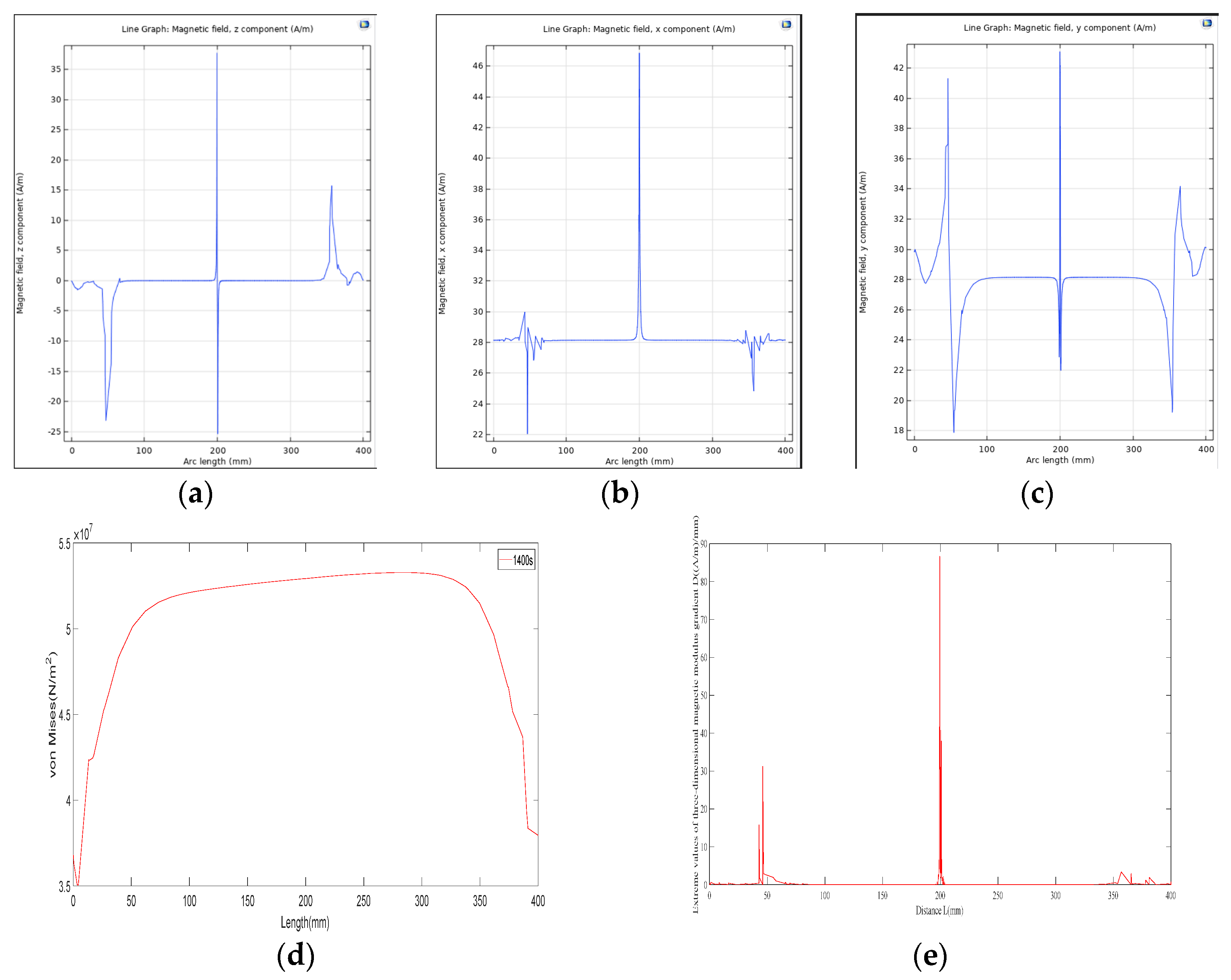
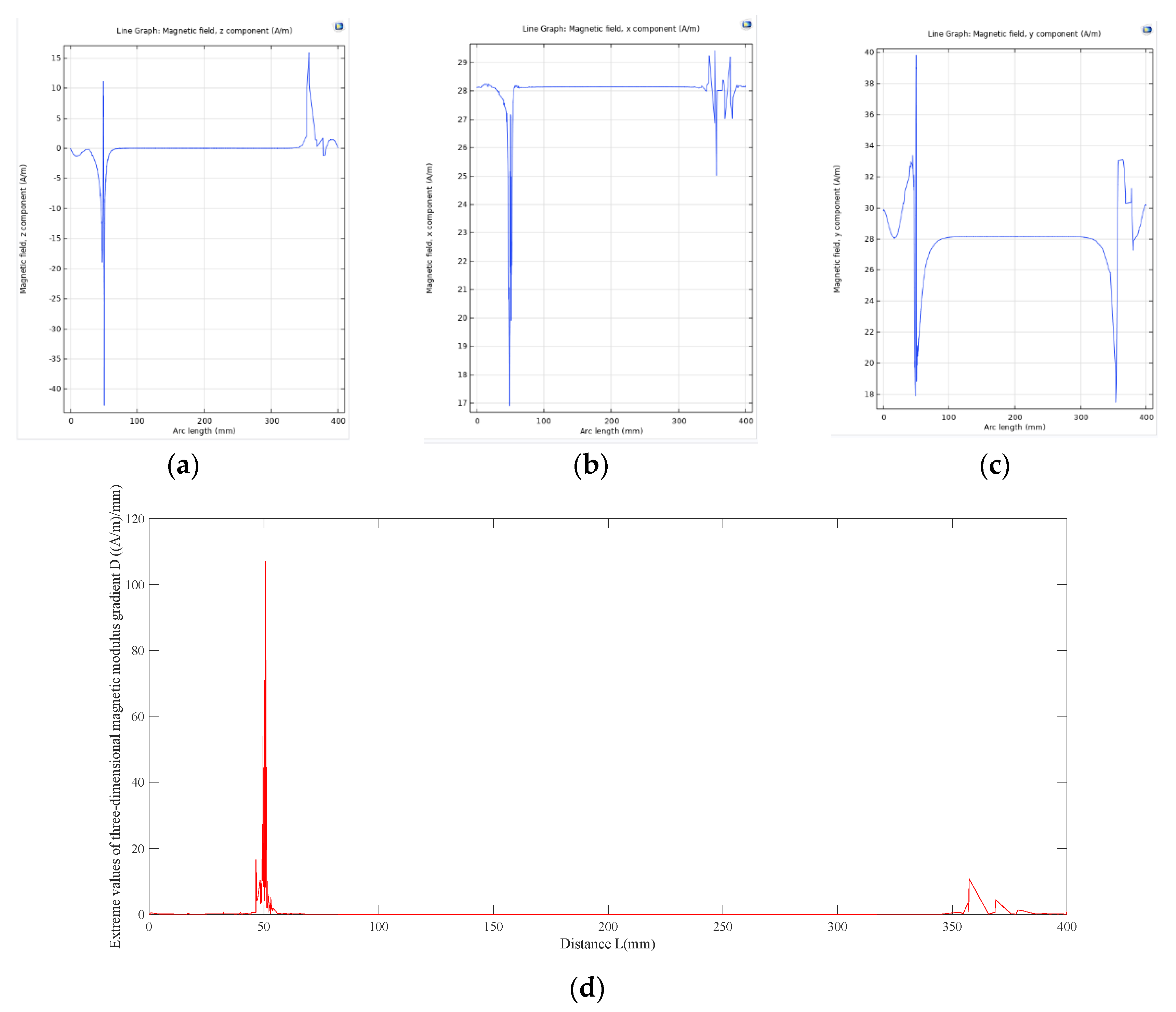
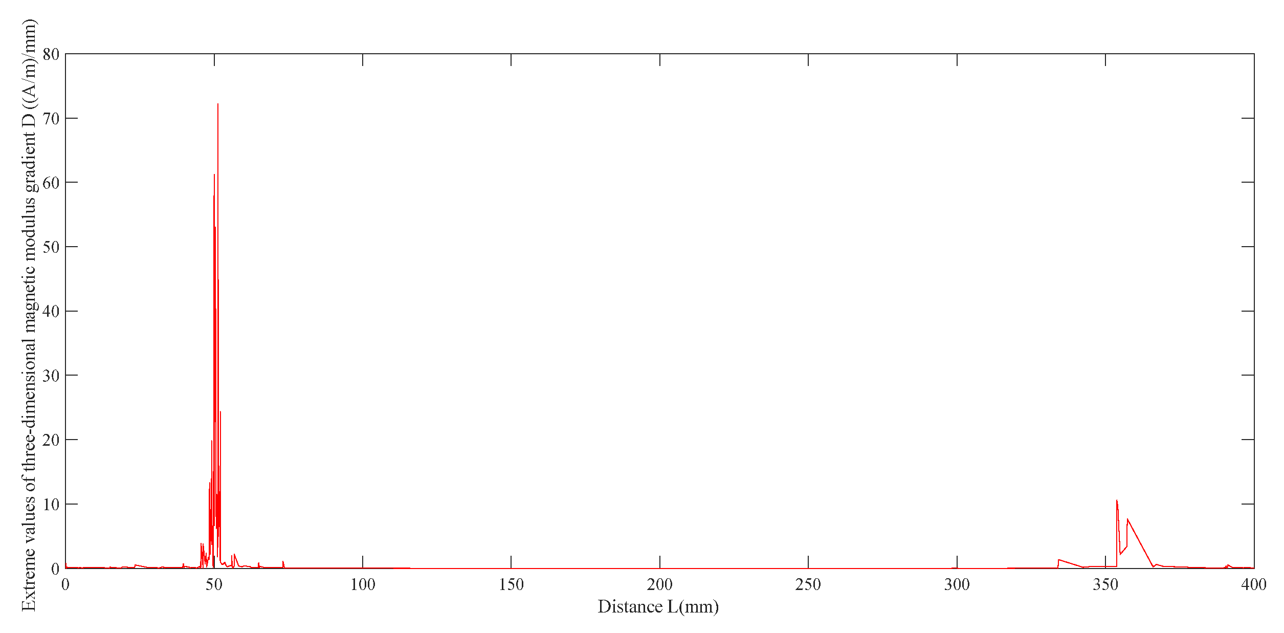
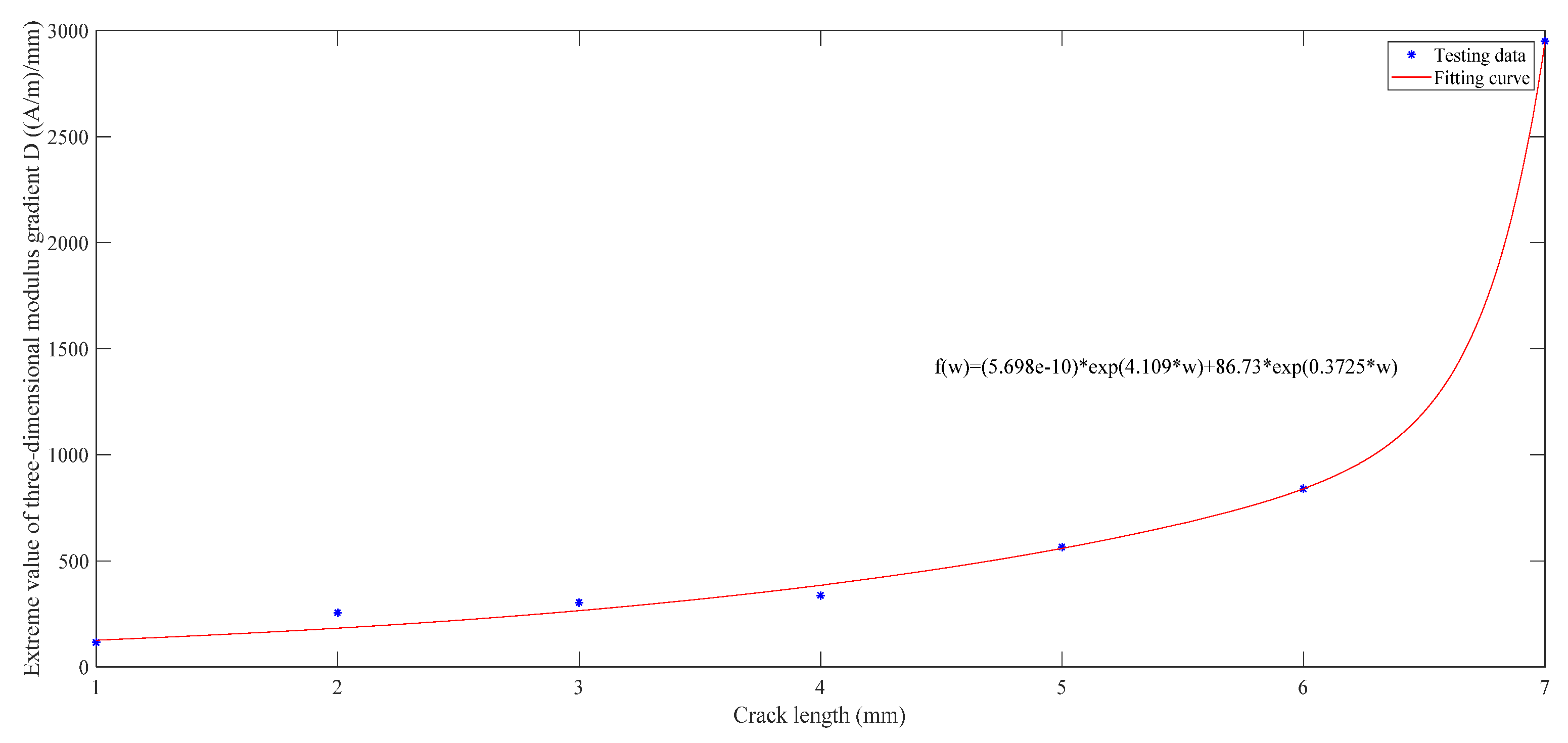
Through COMSOL finite element simulations of welding defects and experimental results of magnetic signals in welding, it can be seen that the three-dimensional magnetic modulus gradient provides good characterization of welding cracks and porosity defects. According to the three-dimensional magnetic gradient, the modulus determines whether the welded components contain welding cracks and porosity-type defects, and determines the length of the defect.
(2)
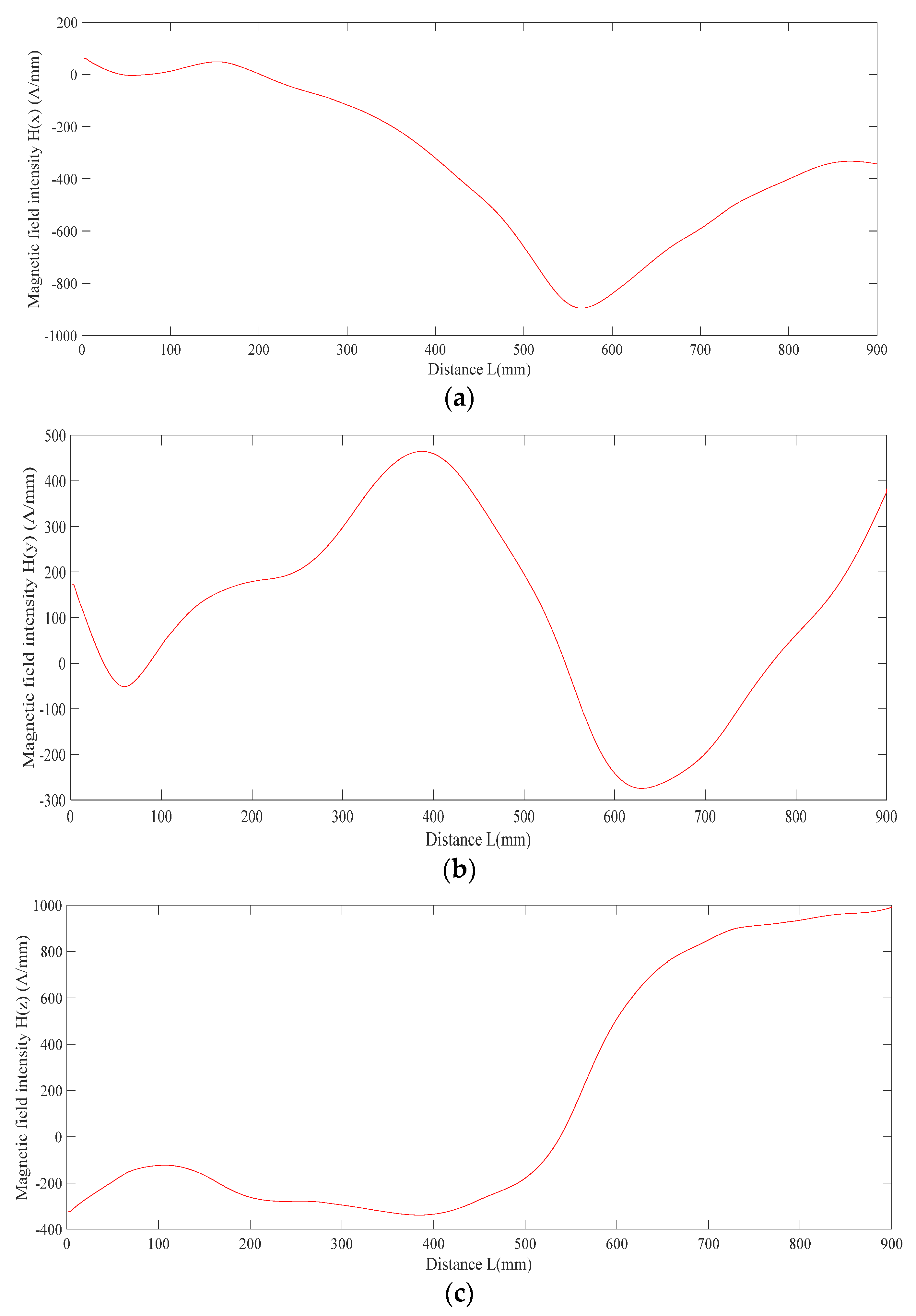
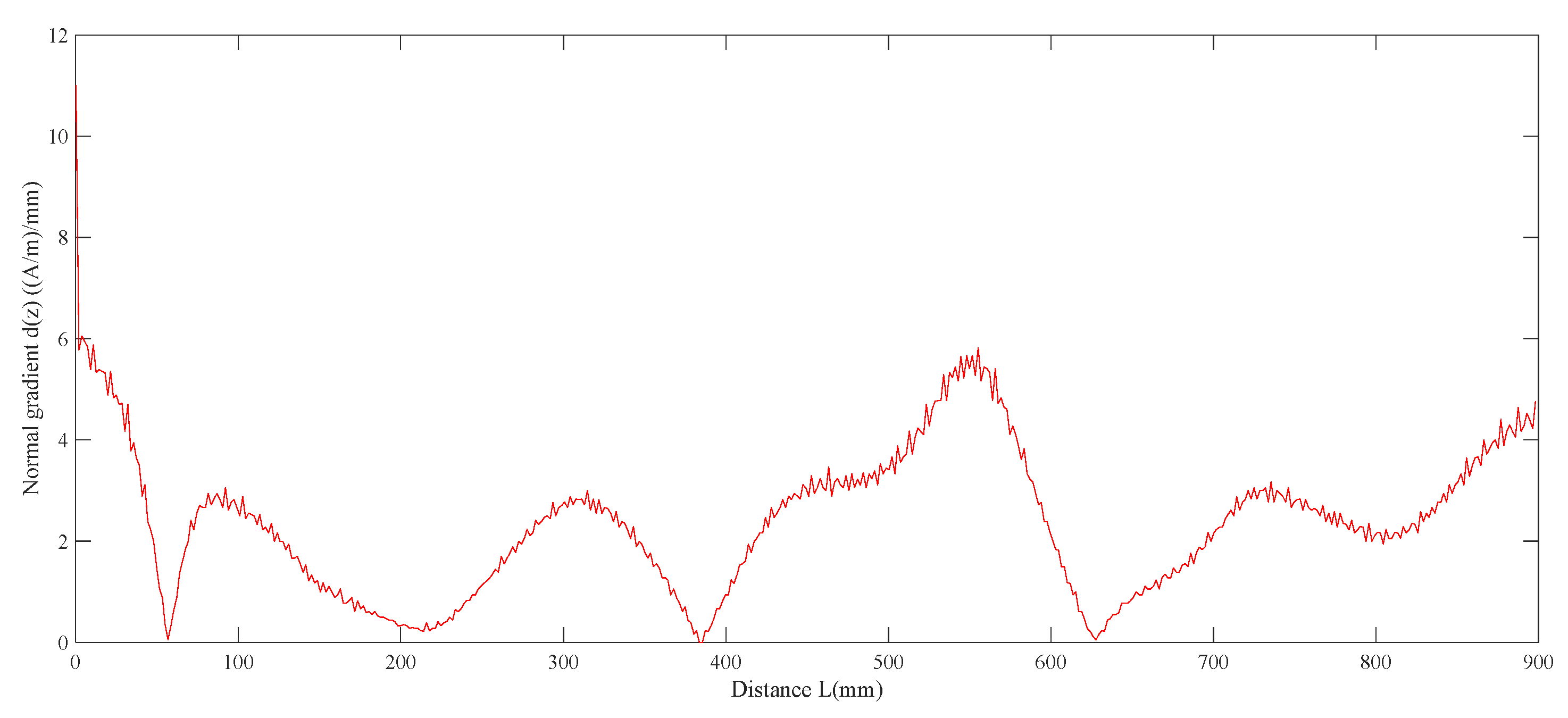
It is clear from the tests that a single normal component gradient pole does not characterize the weld defects well. The three-dimensional magnetic modulus gradient polarity combined with the three-dimensional spatially distributed magnetic signal is a good characterization of the weld defects.
(3)
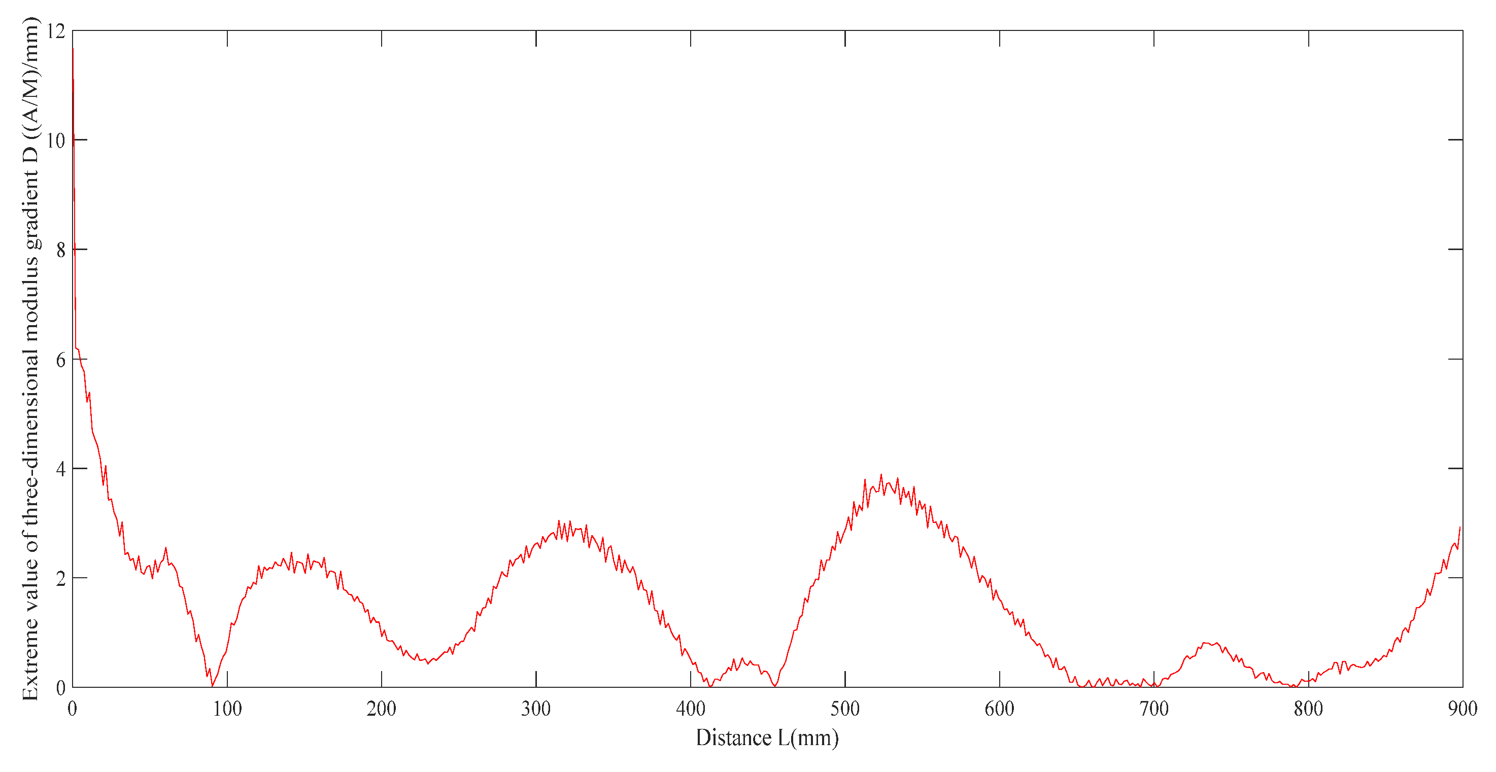
Welding residual stresses and weld cracks and porosity-type defects all lead to changes in the three-dimensional magnetic gradient modulus, but they are fundamentally different. Due to the difference in the degree of magnetic charge build-up and permeability at the defect and the residual stress region, the result is that the magnitude of the three-dimensional modulus gradient is much higher at the defect site than at the residual stress site.
(4)
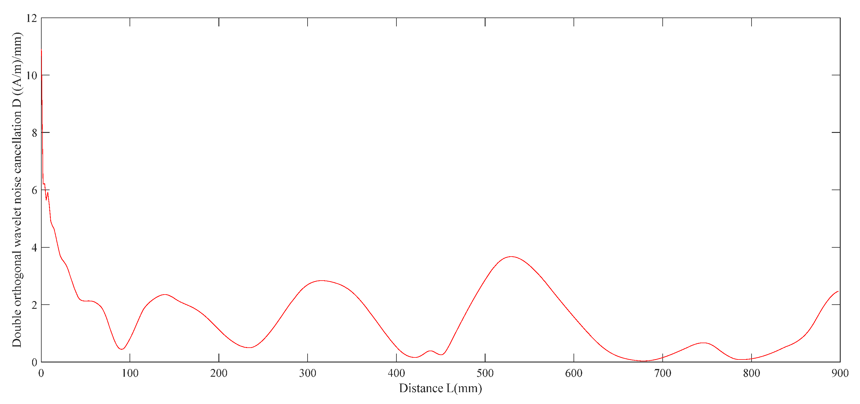
The dual orthogonal wavelet transform method is introduced for the 3D magnetic gradient modulus containing different types of interference noise. The double orthogonal wavelet transform is used to eliminate the strong random interference noise and improve the accuracy of 3D magnetic gradient modulus localization.

Author Contributions

Software, X.P.; Validation, X.P.; Investigation, X.P.; Data curation, L.D.; Writing—original draft, X.P.; Writing—review & editing, Y.C.; Project administration, Y.C.; Funding acquisition, Y.C. All authors have read and agreed to the published version of the manuscript.

Funding

This research was funded by the Natural Science Foundation of Chongqing, China (cstc2019jcyj-msxmX0556).

Conflicts of Interest

The authors declare no conflict of interest.

References

  1. Hu, S.; Ma, L.; Ma, B.; Wei, H.; Zhou, H.; Cen, Y.; Wang, B. Welding process of low density steel and dissimilar steels. Ordnance Mater. Sci. Eng. 2019, 42, 69–73. (In Chinese) [Google Scholar]
  2. Wang, Z.; Sun, K.; Ge, J.; Huang, S. Nondestructive measurement of electron beam weld depth for small diameter tube. Ordnance Mater. Sci. Eng. 2018, 41, 100–103. (In Chinese) [Google Scholar]
  3. Luo, J.; Tan, C.; Li, X. Influence of residual stress on dynamic mechanical properties of welded joints. Ordnance Mater. Sci. Eng. 2022, 45, 31–36. (In Chinese) [Google Scholar]
  4. Liu, C. Detection method of high strength steel structures under pressure-bearing zone. Ordnance Mater. Sci. Eng. 2020, 43, 108–112. (In Chinese) [Google Scholar]
  5. Xu, G.; Liu, T.; Guan, X.; Zhang, X. Analysis of magnetic particle testing and penetrant testing for aviation products. Ordnance Mater. Sci. Eng. 2021, 44, 123–127. (In Chinese) [Google Scholar]
  6. Wang, C.; Zhu, H.; Xv, C.; Yu, W. Application of adaptive wavelet threshold denoising in metal magnetic memory signal processing. Syst. Eng. Electron. 2012, 34, 1555–1559. (In Chinese) [Google Scholar]
  7. Xu, B.S.; Dong, L.H. Metal Magnetic Memory Testing Method in Remanufacturing Quality Control; National Defense Industry Press: Beijing, China, 2015. (In Chinese) [Google Scholar]
  8. Shi, P.P. Quantitative Study of Micro-Magnetic Nondestructive Testing for Stress and Defect in Ferromagnetic Materials. Ph.D. Thesis, Xidian University, Xi’an, China, 2017. (In Chinese). [Google Scholar]
  9. Pandey, C.; Giri, A.; Mahapatra, M.M. On the prediction of effect of direction of welding on bead geometry and residual deformation of double-sided fillet welds. Int. J. Steel Struct. 2016, 16, 333–345. [Google Scholar] [CrossRef]
  10. Taraphdar, P.K.; Kumar, R.; Pandey, C.; Mahapatra, M.M. Significance of Finite Element Models and Solid-State Phase Transformation on the Evaluation of Weld Induced Residual Stresses. Met. Mater. Int. 2021, 27, 3478–3492. [Google Scholar] [CrossRef]
  11. Kumar, R.; Dey, H.C.; Pradhan, A.K.; Albert, S.K.; Thakre, J.G.; Mahapatra, M.M.; Pandey, C. Numerical and experimental investigation on distribution of residual stress and the influence of heat treatment in multi-pass dissimilar welded rotor joint of alloy 617/10Cr steel. Int. J. Press. Vessel. Pip. 2022, 199, 104715. [Google Scholar] [CrossRef]
  12. Rokosz, M. Metal magnetic memory testing of welded joints of ferritic and austenitic steels. NDT E Int. Indep. Non-Destr. Test. Eval. 2011, 44, 305–310. [Google Scholar]
  13. Dubov, A.A. Diagnostics of Boiler Tubes with the Usage of Metal Magnetic Memory; Energoatomizdat: Moscow, Russia, 1995. [Google Scholar]
  14. Yin, D.; Xv, B.; Dong, S.; Dong, L.; Feng, C. Change of Magnetic Memory Signals under Different Testing Environments. Acta Armamentarii 2007, 43, 319–323. (In Chinese) [Google Scholar]
  15. Dong, L.; Xv, B.; Dong, S.; Chen, Q.; Wang, D.; Yin, D. The effect of axial tensile load on magnetic memory signals from the surface of medium carbon steel. Chin. J. Mater. Res. 2006, 46, 440–444. (In Chinese) [Google Scholar]
  16. Gao, Q.; Ding, H.; Liu, B. The Element Simulation and Influence Factors of Metal Magnetic Memory Signals. NDT 2015, 37, 86–91. (In Chinese) [Google Scholar]
  17. Ma, H.; Zhou, J.; He, Z. Experimental study on crack detection of typical butt weld of steel bridge based on metal magnetic memory. Highway 2021, 66, 157–162. (In Chinese) [Google Scholar]
  18. Chen, H.; Wang, C.; Zhu, H. Metal magnetic memory test method based on magnetic gradient tensor. Chin. J. Sci. Instrum. 2016, 37, 602–609. (In Chinese) [Google Scholar]
  19. Chen, H.; Wang, C.; Zuo, X. Research on methods of defect classification based on metal magnetic memory. NDT E Int. Indep. Non-Destr. Test. Eval. 2017, 92, 82–87. [Google Scholar] [CrossRef]
  20. He, G.; He, T.; Liao, K.; Deng, S.; Chen, D. Experimental and numerical analysis of non-contact magnetic detecting signal of girth welds on steel pipelines. ISA Trans. 2021, 125, 681–698. [Google Scholar] [CrossRef] [PubMed]
  21. Ling, T.; Liu, H.; Zhang, L.; Gu, D.; Wu, L. The improved biorthogonal wavelet construction method and its application in blast vibration signal analysis. J. Vib. Shock 2018, 37, 273–280. (In Chinese) [Google Scholar]
  22. Ren, J.; Fan, Z.; Chen, X.; Liu, C. Extraction of Feature Value in Metal Magnetic Memory Testing Based on Wavelet Packet Transform. NDT 2008, 30, 280–582. (In Chinese) [Google Scholar]
  23. Yi, F.; Li, Z.; Su, Y.; Wang, P.; Wu, H. Denoising algorithm for metal magnetic memory signals of oil pipeline based on improved wavelet threshold. Acta Pet. Sin. 2009, 30, 141–144. (In Chinese) [Google Scholar]
  24. Chang, X.; Zhou, D.; Wang, H.; Cao, P. Simulation and experiment on reflection/transmission eddy current for non-ferromagnetic material. Ordnance Mater. Sci. Eng. 2018, 41, 56–60. (In Chinese) [Google Scholar]
  25. Liu, S. 3D Magnetic Susceptibility Imaging Based on the Amplitude of Magnetic Anomalies. Master’s Thesis, China University of Geosciences, Wuhan, China, 2011. (In Chinese). [Google Scholar]
  26. Liu, S.; Chen, C.; Hu, Z. The application and characteristic of a vertical first-order derivative of the total magnitude magnetic anomaly. Highway 2011, 26, 647–653. (In Chinese) [Google Scholar]
  27. Zhong, W. Ferromagnetism; Science Press: Beijing, China, 2017. (In Chinese) [Google Scholar]
  28. Su, S.Q.; Wang, W. Non-Destructive Testing of Building Steel Structure with Magnetic Memory; Science Press: Beijing, China, 2019. (In Chinese) [Google Scholar]
  29. Ren, J.L.; Lin, J.M. Metal Magnetic Memory Detection Technology; China Electric Power Press: Beijing, China, 2000. (In Chinese) [Google Scholar]
  30. Su, S.Q.; Qin, Y.L.; Wang, W.; Ma, X.; Zuo, F. Numerical simulation of stressmagnetization effect for bending states of Q235b steel beam based on magnetic memory. Mater. Sci. Technol. 2020, 28, 11. (In Chinese) [Google Scholar]
Figure 1. Finite element welding model.
Applsci 13 02648 g001
Figure 2. Application of heat source to butt welds.
Applsci 13 02648 g002
Figure 3. Equivalent force distribution for different heat dissipation periods.
Applsci 13 02648 g003
Figure 4. Welding defect components.
Applsci 13 02648 g004
Figure 5. Ultrasonic detection results.
Applsci 13 02648 g005
Figure 6. Three-axis magnetic intensity detection system.
Applsci 13 02648 g006
Figure 7. After 1400 s of heat dissipation. (a) Normal component Z; (b) Tangential component X; (c) Tangential component Y; (d) Equivalent stress distribution; (e) three-dimensional magnetic modulus gradient.
Applsci 13 02648 g007
Figure 8. Defect at 50 mm after 1400 s of heat dissipation. (a) Normal component Z; (b) Tangential component X; (c) Tangential component Y; (d) Three-dimensional magnetic modulus gradient.
Applsci 13 02648 g008
Figure 9. Extreme values of three-dimensional magnetic modulus gradient.
Applsci 13 02648 g009
Figure 10. Variation curve of three-dimensional magnetic modulus gradient with defect size.
Applsci 13 02648 g010
Figure 11. Weld’s magnetic signal diagram. (a) Tangential component X; (b) Tangential component Y; (c) Normal component Z.
Applsci 13 02648 g011
Figure 12. Normal gradient extremum dz.
Applsci 13 02648 g012
Figure 13. Extreme value of three-dimensional modulus gradient of welding defects.
Applsci 13 02648 g013
Figure 14. Double orthogonal wavelet noise cancellation.
Applsci 13 02648 g014
Disclaimer/Publisher’s Note: The statements, opinions and data contained in all publications are solely those of the individual author(s) and contributor(s) and not of MDPI and/or the editor(s). MDPI and/or the editor(s) disclaim responsibility for any injury to people or property resulting from any ideas, methods, instructions or products referred to in the content.

