Abstract
The mechanical simulation experiment can provide guidelines for the structural design of materials, but the module partition of mechanical simulation experiments is still in its infancy. A mechanical simulation contour, e.g., strain and stress contour, has hierarchical characteristics. By analyzing the contour at different layers, the physical properties of the structure material can be improved. Current state-of-the-art methods cannot distinguish between simulation strain contours, as well as sparsely distributed spots of strain (stress concentrations) from simulation strain contour images, resulting in simulation data that does not accurately reflect real strain contours. In this paper, a Hierarchical Tensor Decomposition (HTD) method is proposed to extract hierarchical contours and stress concentrations from the simulation strain contours and then improve the mechanical simulation. HTD decomposes a tensor into three classes of components: the multi-smooth layers, the sparse spots layer, and the noise layer. The number of multismooth layers is determined by the scree plot, which is the difference between the smooth layers and the sparse spots layer. The proposed method is validated by several numerical examples, which demonstrate its effectiveness and efficiency. A further benefit of the module partition is the improvement of the mechanical structural properties.
1. Introduction
The rapid advances in fabrication techniques and the exponential increase in computational power in recent years have enabled researchers to explore new horizons in the fields of material and structural design. Accordingly, module partition [1] can be considered as a powerful numerical tool for optimizing the material arrangement of products at various scales, ranging from nanometers [2] to skyscrapers [3], depending upon the target application. The module partition has different names in different fields; for example, image segmentation [4] and feature extraction [5] are commonly used in the field of image processing. When it comes to mechanical simulation, simulation experiments are usually designed in conjunction with topology optimization [6]. A mechanical simulation using ANSYS [7] is usually required when studying the properties of mechanical structural materials. For accurate calculations of stress and strain fields, meshing is necessary for mechanical simulation experiments by ANSYS [8]. Dense meshes will provide a better representation of the actual stress distribution, whereas coarse meshes will introduce large deviations when it comes to stress concentration [9]. By partitioning the hierarchy of stress or strain contours, we can achieve more accurate simulations of structural materials [1].
Several methods have been developed to incorporate macroscale boundary conditions into the module partition process. For example, the hierarchical design method proposed by Rodrigues et al. [10] is based on the assumption that macroelements represent single-scale microstructures that are optimized iteratively using inverse homogenization, with minimal connectivity effects from points to points at the macroscale due to microstructure configuration variations. A novel optimization approach developed by Huang et al. [11] is based on the assumption that the design space consists of a single designable microstructure whose material layout is optimized based on macroscale boundary conditions. Several researchers have proposed concurrent multiscale module partition to perform module partition at macroscales and microscales simultaneously [12]. An approach called concurrent multiscale topology optimization has been proposed in an attempt to optimize topology at both macro- and microscales [13]. In this method, module partition is performed to obtain both the optimal material layout at the macroscale and the optimal local material distribution at the finer scale.
Various methods are used at macroscales to design partitions for achieving optimal topology, whereas at the local scale, they strive for optimal microstructure, generally by considering uniform microstructures throughout each macrodomain. By considering subdomains within the spatial macroscopic design domain, a grid-based hierarchical approach is applied in this regard, thereby providing the optimal solution that considers uniform microstructures across each macro subdomain [14,15,16]. To optimize macrostructures and microstructures, density-based multipatching has been applied [17,18,19]. Based on proximity or other variables, these methods optimize design at the macroscale. A clustering method based on principal stress/strain directions was developed by Xu and Cheng [20], and a density- and strain-based clustering method were presented by Kumar and Suresh [21]. The macroscale design domain is subdivided into several subdomains by using a dynamic K-clustering strategy based on directions and ratios of principal stresses [22]. It is noteworthy that the K-clustering method used in these works is significantly different from that used in the current thesis in terms of topology optimization. The objective of this paper is to develop a multilayer module partition of the strain/stress contour based on the mechanical simulation by ANSYS in order to guide the improvements of mechanical simulation experiments. Following a brief introduction to the types of mechanical simulation data that are being studied in this paper, a review of the research methods for the different types of data will be provided. Figure 1a depicts a beam having a length of (no particular units) and a height of that is subjected to three concentrated forces having magnitudes of applied at midspan with under plane stress conditions. There are two segments of a beam with a length of , starting at from the beam edges. There are 768 elements in the design space, which is divided into 48 × 16 elements. Figure 1b presents a two-dimensional sample of strain contours of the mechanical simulation data. Figure 1c depicts a three-dimensional sample of strain contours of the mechanical simulation data.
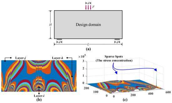
Figure 1.
A hierarchical mechanical simulation strain contours with different layers. (a) is the design domain and boundary conditions; (b) is the strain contour for (a) by ANSYS; (c) is the three-dimensional display of (a).
Such mechanical simulation data by ANSYS with the following characteristics: (i) Multilayer, i.e., smoothness background/foreground layers, as shown in Figure 1b: a background layer of a globally smooth (continuous and differentiable) whole region that spans the entire area of the tensor/matrix/image, filled with low-/medium-intensity elements. The foreground layers with locally smooth regions that span subareas of the tensor, filled with high-intensity elements that are different from the surrounding background; (ii) a spot layer of sparsely distributed small rugged areas filled with high-intensity elements that are significantly different from the surrounding background and/or foreground, as shown in Figure 1c; (iii) Measurement uncertainty: inconspicuous sparse spots or low signal noise rate (SNR) components are easily submerged in measurement data. A layer of noise spans the entire area of the tensor with independent elements of low intensity.
Those layers, i.e., smoothness background/background, spot, and noise layers, of an image/two-way tensor collected from the mechanical simulation data specific “image structural properties” [23], which make the decomposition possible. Smooth background layers are characterized by low-intensity pixels and low gradient variations. The foreground layer is defined by the boundaries of a large gradient that contrast the high-intensity subregions from the surrounding low-intensity background. The internal areas of the foreground are continuous and smooth, characterized by high-intensity elements with low gradient variation. The spots layer sparsely distributed in an image is formed by the stress concentration. The internal areas of spots are small and nonsmooth, characterized by high-intensity elements with high gradient variation.
In numerous studies, foreground cluster regions have been extracted from images, and/or sparse spots have been detected without necessarily distinguishing foreground clusters from spots. For foreground cluster and/or spot detection, the currently available state-of-the-art methods generally employ a mapping of the image characteristics of the different components with mathematical characteristics of the different model components, such as smoothness and sparsity. The separation of foreground from the background has been demonstrated in several studies through the determination of different intensity components from a two-way matrix or tensor but without explicitly distinguishing between foreground clusters of intensities and sparse areas. Methods such as local thresholding [24] and global thresholding [25] are employed to separate background and foreground data. The original data can then be separated into foreground and background using Otsu’s method [26]. It should be noted, however, that the simplest implementation of the algorithm yields only one intensity threshold, which is used to classify elements into two classes. There is no bimodality in the histogram of the original data if the clustered regions in the foreground are less large than the areas in the background [27]. Based on a single global threshold that minimizes variations in intensity within foreground clusters within an image, global thresholding approaches organize the elements in an image into two foreground clusters, a background cluster, and a foreground cluster. There are several techniques developed to overcome this problem, for example, adaptive thresholding segmentation [28] and maximum entropy threshold segmentation [29]. By assessing the relative intensity levels of elements in the local area, local thresholding establishes the boundary between foreground and background. Using a global thresholding approach for extracting foreground cluster features and segmenting objects from an image with multiple components, may result in excessive variation of intensity within a foreground cluster, making it difficult to distinguish between the features of individual regions from the background [30]. However, if the components of different types overlap in the foreground, local thresholding approaches with multiple thresholds may be merged. Defining thresholding-based solutions as an approach has a fundamental problem in the fact that they do not explicitly take into account the smoothness and sparsity of tensor structures, as well as the characteristics of the components in the raw data when setting a threshold, and as a result, they are not able to efficiently decompose tensors. In the analysis of data and the reduction of dimensionality, low-rank-based decomposition methods [31] have become widely used. The principle is based on the assumption that an image can be decomposed into a low-rank component, which lies within a low-rank subspace, and a sparse component. In addition to repairing images and recognizing objects, this method can be used to reconstruct data, detect small targets, and identify data sources [32]. There are a number of proposals for separating low-rank and sparse components from the original data, such as Robust Principal Component Analysis (RPCA) [33]. After this, several methods are proposed based on RPCA. As one example, the researcher composed a low-rank matrix and sparse component recovery problem [34] to detect the sparse spots in the infrared image. A spatially weighted PCA formulation [35] was developed to improve the local correlation structure. A low-rank component, which contains information about the smooth background and partial foreground of the background, is a component that contains two similar points: (i) represents the span of two vectors with linear correlation; (ii) sparse spots, which represent rugged areas of high intensity that are sparsely distributed. Considering the two points cited above, the low-rank decomposition method does not explicitly distinguish between the global and local smoothness of the foreground and background, respectively. Therefore, it is inapplicable for determining the foreground cluster regions’ features.
Many methods can be derived from functional analysis, including kernel smoothing, SVD decomposition, Fourier transformations, wavelet transformations [36], and B-spline [37] transformations. These approaches are mostly used in order to eliminate noise from the original data. The detection of defects (sparse spots) makes use of a number of approaches, including derivative operators, Laplacian operators, and Sobel operators. The methods described above, however, may not be able to simultaneously estimate the different foreground cluster regions and sparse spots due to their lack of detection accuracy and computation time. Smooth-sparse decomposition (SSD) [37] is proposed as a method for identifying sparse anomalies (sparse spots) in images. A Smooth-Sparse Decomposition model is developed in order to explore the spatial-temporal properties of images. The model is referred to as Spatial–Temporal Smooth Sparse Decomposition (ST-SSD) [38]. A smooth background, sparse anomalies, and noise are assumed to be present in every image, regardless of whether it is on a SSD or ST-SSD. If the distinct foreground cluster regions and sparse spots must be distinguished, these approaches based on functional analysis may not be applicable. As a consequence, SSD and ST-SSD suffer from a major disadvantage, which is the assumption that sparse spots on each point are independent. The penalized nonparametric regression model [39], which mainly focuses on sparse spots detection, is proposed in order to capture the spatial–temporal structure of tensor data and detect anomalies. As a result, if an original dataset contains a combination of foreground clusters and sparse spots at the same time, these components cannot be separated completely.
Images are decomposed using tensor-based methods in which each entry corresponds to an intensity value. As opposed to modeling an image with surrogated basis functions, these methods decompose an image into a tensor. The original structure of the image is preserved without any loss of information. Many research approaches have been developed for the analysis of sequence images today. Some of these approaches include low-rank tensor decomposition [40,41], CANDECOM/PARAFAC (CP) decomposition [42], and Tucker decomposition [43]. The decomposed component vectorization is performed for the low-rank tensor decomposition. A substantial portion of the feature information will be lost as a result of discarding the residuals of the decomposition. In the case of the CP decomposition, the correct rank and global minimum error are nondeterministic polynomial time problems [42], which are not determinable. CP decomposition has an unknown number of layers. Tucker decomposition also produces an unpredictable result, especially if the core tensor is dense. Because of this, these methods cannot be used to identify important features within an image, such as foreground clusters or sparse areas.
In this paper, a novel, module partition method is pursued, i.e., HTD model. Following is a summary of the remaining content of the article. The proposed methodology is then presented in Section 2. In Section 3, we present a simulation study that evaluates the performance of the proposed method. The proposed method is evaluated against benchmark techniques in Section 4 through the use of a case study. In Section 5, we conclude with a discussion of future directions.
2. Proposed Methodology
To extract more information from a two-way tensor, a HTD method is presented in this section. HTD decomposes a tensor into several smooth and sparsity components. Detailed descriptions of the above components are provided in the following parts.
2.1. Decomposition Model
The purpose of this subsection is to introduce the model of decomposition and propose an efficient algorithm to implement it. As shown in Figure 1c, strain contours are employed, with a global smooth background, several local smooth foregrounds, and sparsity spot strains (caused by concentrations of stress). The global smooth background has low intensity variation. The sparsity spot strains have high intensity variation. The local smooth foregrounds have greater intensity variation and are occupied in a greater proportion than sparsity spot strains. Random noise is embedded in the sample. Simulated strain contours (tensors) have a few common characteristics, including a smooth background layer, several smooth foreground layers, sparse spots, and noise layers.
Assumption a two-way tensor , it could be modeled as a linear superposition of background component , foreground components , sparse spots (), and noise component, which can be formulated as , where , , , , , and , represent the input data, background layer, foreground layers, sparse spots layer, and noise layer, respectively. The size of is , with its th element, , the intensity of the corresponding point in the tensor, and and , and . It can be decomposed to a smooth background layer , several foreground layers , a sparse spots layer , and a noise layer , respectively. The smooth background component, , consists of elements with low intensity variation and span whole space in tensor data. The foreground layers, , comprise of several high intensity variation smooth foreground cluster regions, and from to , the region occupied by the foreground cluster regions of high intensity variation becomes smaller and smaller. Compared with the background and foreground, the sparse spots layer, , consists of a large amount of zero-value elements, high-value elements, and the largest intensity variation. The residual, E, represents the noise and the unmolded errors, which is assumed to be independently and identically normally distributed, i.e., .
A gradient at a particular element is composed of two horizontal and vertical gradients, which are a set of horizontal and vertical gradient bases, respectively. , , …, , …, and are first-, second-, …, th-, …, and th-order difference matrix [23,37].,
where , , ; , , where .
The difference matrices are employed to calculate gradients of discrete variables such as: a first-order difference matrix operator is ordinarily employed to calculate the gradient change between adjacent points of a vector; a second-order difference matrix operator is ordinarily employed to calculate the gradient change between adjacent points; a N-order difference matrix operator is ordinarily employed to calculate the gradient change between two n − 1 adjacent points. As a consequence, components with different characteristics of intensity variation may be derived from the original data by employing various difference matrices. Thus, taking into account the hierarchical characteristics of a two-way tensor, its magnitude can be given as , where is tuning parameter, is the Frobenius norm [44].
Least square regression is used to estimate the model components (i.e., and ). To ensure the smoothness of the estimated back-/foreground and the sparsity component, the least square loss function is augmented by l1 [45] and Frobenius norm penalties, which results in the following penalized regression criterion:
where are tuning parameters, which control the tradeoff among background, foreground, and sparse spots; is determined the gradient magnitude. The intensity variation of the background and foreground can be guaranteed by combining , and the corresponding different order difference matrices. The sparse spot layer is controlled by . Finally, sparse spots , which should have been calculated by l0 [45], i.e., ; however, the optimization is an NP-hard problem [46,47], through replacing it with a convex surrogate to make the above problem tractable.
According to Equation (1), all components including background and foreground and the sparse spots layer () can be determined. Consequently, the performance of the proposed method is assessed by comparing the estimated components with the ground truth components. In this study, a criterion is introduced, which is the root mean square error (RMSE), for computing the intensity of all elements between the estimated components and ground truth components.
2.2. Performance Indicators
Anomalies [37] and small targets [34] are all terms used in different fields to describe sparse spots. All of these systems have one characteristic in common, namely the binarization of element intensity into 0–1 classes. Detailed binarized representations of each element of the sparse spots layer are provided in order to facilitate analysis. Ground truth for the sparse spots layer indicates that each element of the spot will be regarded as 1, and any other element will be regarded as 0. All elements that do not equal zero constitute an estimated sparse spot layer. In this case, the elements will be treated as sparse spot elements and will be set to 1. A binary classification problem is involved in the detection of the intensity of each element in the sparse spots layer; therefore, two types of general misclassification are considered in this study: False Positives and False Negatives.
Definition 1.
False Positive (FP) is defined as the total number of elements that are incorrectly classified as the sparse spots layer while these elements actually belong to the background and foreground, i.e., , where is the indicator function.
Definition 2.
False Negative is defined as the total number of elements that are incorrectly classified as the background and foreground while these elements actually belong to the sparse spots layer, i.e., .
Definition 3.
True Positive (TP) is defined as the total number of elements that are correctly classified as the determinate foreground cluster regions or sparse spots while these elements actually belong to the corresponding foreground cluster regions layer or sparse spots layer, i.e., .
Definition 4.
Root Mean Square error (RMSE) is defined as the average of the absolute differences between the estimated value of each element in the estimate and that of the corresponding element in the true component, e.g., .
2.3. Optimization Algorithms for HTD
A convex loss function can be solved using the Alternating Direction Method of Multipliers (ADMM) [48], as shown in Equation (1). HTD is defined as a linear combination of several convex regularization terms that satisfy the ADMM assumption. As part of its goal, the ADMM algorithm aims to minimize the sum of a group of convex functions that are constrained. The augmented Lagrangian for Equation (1) is defined as
where is the Lagrange multiplier matrix, , is the outer product operator, and is a positive penalty scalar. With the increasing number of iteration steps, becomes smaller, which leads to a suppression of residual and improves the performance of the ADMM algorithm. ADMM initializes , where . Then, with solved at iteration k, the solution at iterations can be split into separate problems, each of which can be solved in parallel. Explicitly, , in Equation (2), is updated by with the other terms fixed, which results in
where .
Then, , where is an identity matrix. It can be written as Sylvester equation [49] : , where , , and . Then, it can be solved. , in Equation (2), is updated by with the other terms fixed, which results in
where .
Then, the solution of the proposed HTD is given in Algorithm 1.
| Algorithm 1 Hierarchical Tensor Decomposition Method |
| Input: |
| Initialization: |
| while not converged do |
| Step 1: Updating with the other items fixed by |
| Step 2: Updating with the other items fixed by |
| Step 3: Updating with the other items fixed by |
| Step 4: Updating with the other items fixed by |
| Step 5: Updating by |
| Step 6: Check the convergence condition |
| Step 7: Updating k |
| return. |
Upon convergence of the algorithm, , and can be estimated. An element in the tensor, i.e., , is classified as the sparse spots if the estimated sparse spots layer at the same location, , is not equal to zero, as
There are few elements with high magnitudes of intensity in the foreground layer since the foreground layer is characterized by high-intensity variations. To ensure a smaller , as many elements as possible will have a similar intensity value. The areas covered by elements with high intensity variations are often smaller than those covered by elements with low intensity magnitudes. Two adaptive thresholds [50] are introduced to segment these regions with large intensity variations from the foreground layers, i.e.,
where and are the mean value and standard deviation of the foreground cluster regions layer , respectively; , and are constants determined empirically. An element satisfying is considered when the region to be detected in has a higher intensity value than the background. For the region to be detected and the background has a lower intensity value, the element corresponding to is selected.
2.4. Layer Determination and Tuning Parameters
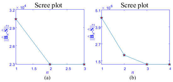
A tensor is divided into four layers based on the different intensity variations: the background, the multilayer foreground, the sparse spots layer, and the noise layer. As the number of layers increases, the intensity variation of the extracted foreground cluster regions layer increases. is decreasing and gradually decreases with the increase of the number of decomposition layers. Therefore, it can be used to derive the number of background and foreground layers. When and are approximately equal, the number of foreground cluster regions layer can be determined to be n. Scree plot [51] of is introduced. In multivariate statistics, the scree plot is a line plot of the eigenvalues of factors or principal components in an analysis. A scree plot always displays the eigenvalues in a downward curve, ordering the eigenvalues from largest to smallest. It is believed that significant factors or components to the left of the “elbow” of the graph are to be retained in the scree test because the eigenvalues appear to level off at this point [52]. Nevertheless, we found that the scree plot can be utilized to determine the number of foreground cluster regions layers. An intuitive scree plot will be presented in the next section of the simulation experiment in order to illustrate the problem of determining the number of layers more intuitively.
There are tuning parameters in the HTD method, i.e., and . As previously mentioned, is used to control the intensity variation of the background, and is used to control the sparsity of the sparse spots layer.
A tuning parameter can be classified into two categories: (i) ground truth is available and (ii) ground truth is not available. Given a training data , and the corresponding ground truth , , , which is the foreground cluster regions layers, sparse spots layer, and noise layer of , the optimal tuning parameters can be determined by minimizing the error [53]:
where is the tuning parameter, represents the difference between the ground truth and the estimated. There are two scenarios that should be interpreted. One scenario is when each element in each layer has a corresponding intensity ground truth, , where ; and are the estimated of the background and foreground, sparse spots, respectively; another one is that each element is a 0-1 classification problem, e.g., sparse element as a defect object should be detected, .
As there is no training sample to analyze, the choice of should be made empirically based on the structural assumption and the feature to be extracted. A larger is used in adjusting the parameters, which suppresses the estimated variable. There are more than three parameters involved in the model, such as , and , which should be tuned. Therefore, the control variable method should be utilized when tuning the parameters. Specifically, when tuning , it is recommended that , and are fixed until has been determined to be optimal. After that, an optimal is determined. Finally, should be tuned by fixing , until the optimal has been established. In addition, is used to control the variation of intensity of the background and the foreground, and its adjustment can be combined with the actual physical meaning. contribute to determining the smoothness direction. As a result of a large , there will be low intensity variation. is tuned to identify sparse defects. Consequently, when is reduced to a small value, a false negative may occur, e.g., large intensity values of noise may be identified as sparse defects. Increasing may result in some smaller defects being lost. In this context, and should be selected and tuned based on the physical significance of their respective components.
3. Simulation Study
To evaluate the effectiveness of the proposed HTD method under various conditions, several simulation samples are used in this section. Initially, two samples are simulated with different intensity variation layers within foreground cluster regions in order to demonstrate how to determine the number of layers. As illustrated in Figure 2 and Figure 3, these tensors contain different layers of foreground cluster regions and sparse spots. Both of these simulation samples correspond to two-way tensor based on the following model: , where represents the background and foreground cluster region layers, , represents the sparse spots layer, and represents random noise. Specifically, Figure 2 is composed of a background layer , a layer with foreground cluster regions , a layer of sparse spots (, and a layer of random noise (). Figure 3 consists of a background layer , two layers with foreground cluster regions , a sparse spot layer , and a random noise layer (). Essentially, is created by merging multiple two-dimensional Gaussian distributions. The centers of these two-dimensional Gaussian distributions are randomly distributed in the area of . The intensity variation of is determined by superimposing these two-dimensional distributions. With such simulation constraints, can be guaranteed to vary smoothly and with a certain intensity variation. With the increase of n, the intensity variation of increases gradually. In Figure 2, is simulated by the superposition of 8 two-dimensional Gaussian distributions; is generated by a two-dimensional Gaussian distribution. In Figure 3, is generated by the superposition of 10 two dimensional Gaussian distributions; is generated by a two-dimensional Gaussian distribution; is simulated by a two-dimensional Gaussian distribution. A sparse spots layer is simulated to model the sparseness of . This layer consists of several small, connected, closed areas that are tightly connected. It is noteworthy that each area includes a square of elements, and its intensity variation is relatively larger than that of . Finally, each element in the noise layer follows a Gaussian distribution , where .
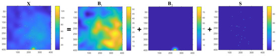
Figure 2.
The simulation data with two smooth layers, sparse spots layer, and a noise layer and the scree plot of the simulation data.
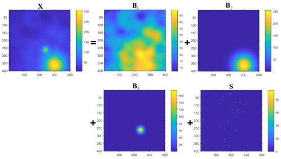
Figure 3.
The simulation data with three smooth layers, sparse spots layer, and a noise layer and the scree plot of the simulation data.
To determine the number of layers of decomposition, the simulation data from Figure 2 and Figure 3 were first decomposed using the proposed HTD method. Then, the scree plot was used to determine how many layers of decomposition there were. The decomposition of the tensor with multilayer property is accomplished by determining the number of layers based on domain knowledge and evaluating the variation of , as shown in Figure 4. For the simulation in Figure 4a, , where . Referring to the simulated data , when , ; therefore, the number of the smooth layer of is . As a result, is divided into three components, , , and . For the simulation in Figure 4b, when , ; therefore, the number of the smooth layer of is . As a result, is divided into four components, , , , and .
In order to demonstrate the good performance of the HTD method, we compare and analyze the simulation data in Figure 2 against the four existing methods, i.e., the Niblack local thresholding SSD, RPCA, and CP decomposition. All the algorithms were coded in MATLAB R2020a and run on a desktop with a CPU of i7 9750H, RAM of 16 GB, and GPU of RTX2060. As shown in Figure 5a–e, the green solid wireframe represents the decomposed result for HTD, local thresholding, RPCA, SSD, and CP decomposition, respectively. The proposed HTD method is clearly superior to other benchmark methods in terms of performance. Evidently, the intensity variations of , and , in Figure 5a, are approximately equal to the ground truths for the corresponding components. For example, in Figure 5a, the color bar for is about (20, 45), and the ground truth is about (15, 50); the color bar for is about (0, 50), and the ground truth is about (0, 70); the color bar for is about (0, 80), and the ground truth is about (0, 80). In Figure 5b, the local thresholding method mixed the background with high-intensity variation areas, foreground cluster regions, and sparse spots into one component. The poor performance of this method is because it is sensitive to the local window size, the bias [24], and noises. In Figure 5c, the extraction shows reasonable performance, and the intensity variation corresponds well with the ground truth; however, the foreground cluster regions and sparse spots are combined into one component. This issue was caused by the SSD identifying regions with high intensity variations as anomalies. According to Figure 5d, the background and foreground cluster region are merged into the extraction component . The reason for such a problem is that a low-rank two-way tensor is the sum of two-way tensors formed by the outer product of two orthogonal vectors. Therefore, data with a low rank property does not demonstrate smoothness and low intensity variation features. Furthermore, the intensity variation depicted in Figure 5d is sensitive to noise with high-intensity values. In Figure 5e, the CP method is used to decompose the simulation data into four components, and each component has a linear relationship between the rows and columns. However, the CP method cannot interpret the relationship between extraction components and ground truth.
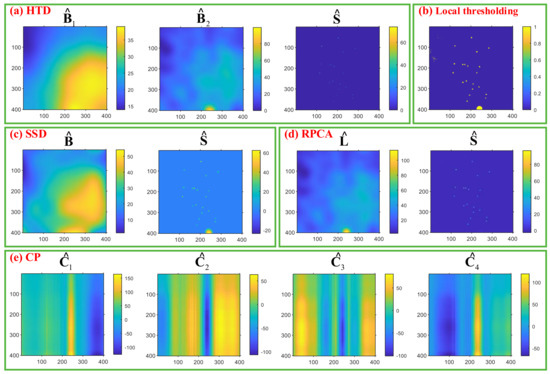
Figure 5.
Results of the simulation data using the proposed method and benchmark methods.
In qualitative analysis, as previously mentioned, the proposed algorithm is superior to the benchmark methods. To more effectively illustrate the performance of the proposed algorithm, Precision, Recall, and F1 are introduced.
Precision is defined by the TP and the FP, as . Recall is defined by the TP and the FN, as . Precision evaluates the percentage of correct component extraction among all elements that are classified as a correct component by the proposed method. Recall evaluates the percentage of all the actual component elements that are correctly extracted. The Recall is sensitive to the FP, whereas Precision is sensitive to the FP. To evaluate the overall performance of the proposed method for deterministic component extraction, the F1 score is introduced. This score is determined by taking the harmonic mean of the Precision and the Recall, as .
The four existing methods and the proposed HTD method are applied in simulated data, as shown in Figure 2, to extract the foreground cluster region and sparse spots from . The region of foreground clusters and sparse spots is labeled in Figure 6a,b, respectively, where the yellow section represents the foreground cluster region, the green sections represent the sparse spots, and the blue section represents the background with noise. The RMSE, Precision, Recall, and F1 score of the proposed HTD, Local thresholding, RPCA, and SSD methods are reported in Table 1. According to Equation (3), the elements belonging to sparse spots in are extracted and binarized.
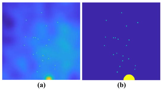
Figure 6.
Simulation data, labeled foreground cluster region and sparse spots. (a) is simulated data; (b) is labeled foreground and sparse spots.

Table 1.
The Precision of the decomposition result is based on the proposed HTD method.
Given TP, the Precision is determined by FP. Low Precision indicates a high FP, which means few sparse spots are correctly categorized as sparse spots. Consequently, a higher Precision algorithm is preferred. Similarly, given TP, the recall is determined by FN. Table 1 depicts the local thresholding method’s superior performance in recall, but poor performance in precision. It is primarily due to its heightened sensitivity to large amounts of noise. Additionally, local thresholding using multiple thresholds may result in a mix of foreground cluster regions and sparse spots, as shown in Figure 7a. In Figure 7b, the highlighted green regions on are extracted sparse elements based on SSD. SSD models the background and the sparse component with basis expansion. As shown in Figure 5c, the basis function, such as a B-spline basis, smooths the background . Then, the RMSE of is computed as . However, there was a false identification of the surrounding areas as part of the sparse component, which included foreground cluster regions and sparse spots. This caused low precision. Based on HTD, the background and foreground cluster regions layers are decomposed from . and are calculated, as shown in Table 1. To extract the foreground cluster region, the postprocessing of is applied based on Equation (4). The region to be detected in has a higher intensity value than the background. Therefore, the element satisfying is considered as foreground cluster element. , . Table 1 demonstrates that the RPCA achieves a better precision for sparse spot extraction; however, its recall requires to be improved. This is because RPCA is sensitive to the high-intensity value element. It is more clear, as shown in Figure 7c, that the extracted sparse elements by RPCA are highlighted with green color on . As shown in Figure 8, the proposed HTD extracts the foreground cluster region and sparse spots with the most efficient performance, among all the methods.
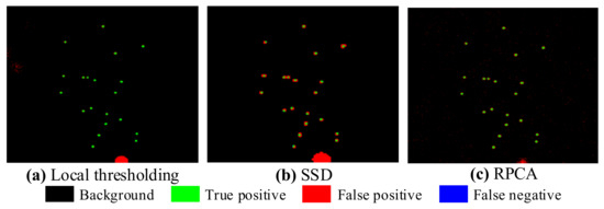
Figure 7.
The extracted sparse component based on local thresholding, SSD, and RPCA.
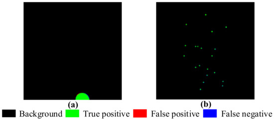
Figure 8.
The foreground cluster region layer and sparse spots layer extracted by the proposed HTD method are compared with the labeled ground truth. (a,b) are the foreground cluster region and sparse spots, respectively, extracted by HTD.
4. Case Study
In this section, the proposed HTD method is applied to a case study of the module partition of the mechanical simulation. First, as part of the proposed method, the scree plot of is used to determine the layer of decomposition, as shown in Figure 9. When the raw data is divided into three layers, , which indicates the number of layers should be determined to be two. Then, the proposed method and the benchmark methods are applied to the raw data. As shown in Figure 10a, it is evident that the HTD algorithm provides a background layer, a foreground layer, a sparse spots (stress concentrations) layer, and a random noise layer. Among these layers, the background layer has low intensity variation, the foreground cluster region layer has higher intensity variation than the background layer, and the sparse spots layer has a higher intensity variation than the foreground layer. Local thresholding is sensitive to sparse spots and noise, resulting in large detection errors, as shown in Figure 10b. SSD decomposed the raw data into three components, i.e., smooth background, sparse, and noise components. It can be seen in Figure 10c, the foreground cluster regions are divided into the sparse component. The low-rank method combined the foreground layer and the background layer into one-layer , which also included a partial sparse stress concentration feature, as shown in Figure 10d. Figure 10e shows the result of CP decomposition method. Though CP decomposition can separate raw data into layers, each layer is the outer product of the two one-way tensors, which makes the decomposition layer difficult to interoperate according to the physical meaning.
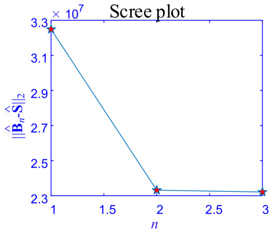
Figure 9.
The scree plot of the strain contours of the mechanical simulation sample.
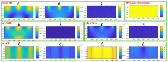
Figure 10.
Results of the case study using the proposed method and benchmark methods.
According to Equation (3), the elements that belong to sparse spots in are extracted and binarized. A postprocessing method based on Equation (4) is applied in to extract the clustered foreground regions. The region to be detected in has a higher intensity value than the background. Therefore, the element satisfies is considered as foreground cluster element. , . The foreground cluster and sparse stress concentration detection result of , and RPCA are labeled, after postprocessed and , as shown in Figure 11. In Figure 11a, the foreground cluster regions are detected and marked as red color, the sparse stress concentrations are labeled as green color. As shown in Figure 11b, noises with high intensities have been identified as stress concentrations, primarily as a result of their high intensity. For SSD, the background and foreground cluster regions are divided into one layer, the sparse stress concentrations are identified as shown in Figure 11c the majority of foreground regions and sparse stress concentrations are not detectable. RPCA is sensitive to the high-intensity value noise; there are many FP elements, as shown in Figure 11c. Obviously, the proposed HTD method has a better performance than the benchmark methods.
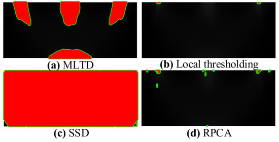
Figure 11.
The detection result of the foreground cluster regions and sparse stress concentrations based on the HTD, Local thresholding, RPCA, and SSD.
To improve simulation results, the stress concentration and strain cluster regions were extracted by the HTD method. By increasing Young’s modulus from 2 to 3 in the red region of Figure 11a in the simulation, the amount of deformation is reduced by 25% as illustrated in Figure 12a for the original simulation result and Figure 12b for the improved simulation result. It is evident that the maximum strain value decreases from to .
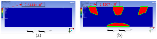
Figure 12.
Simulation result by ANSYS, (a) Young’s modulus = 2; (b) Young’s modulus = 3 in red regions.
5. Conclusions
The partition of foreground cluster regions and sparse spots in strain contours of the mechanical simulation is crucial for improving their structural properties. Based on the ANSYS used in the mechanical simulation process, in this paper, we propose a method to extract layers with background, foreground (partition regions), and sparse spots layers, respectively, from two-way tensors with a noise layer. In particular, multiple smoothing regularizes are developed to extract various intensity variations in the background and the foreground. The norm is introduced to separate the sparse spots (stress concentrations) with high intensity variation from the raw data. The regularization tensor decomposition method is solved using the ADMM by updating each component iteratively. A simulation was conducted to evaluate the proposed HTD’s performance and compare it to some existing methods in terms of element- and object-level detection. Taking into account the simulation results, it can be concluded that HTD outperforms other benchmarks. Moreover, to determine the number of layers in the HTD, the scree plot is used. The proposed method is applied in a real-world case study and the results show its superiority by comparing with other benchmark methods. Further extension of the proposed HTD algorithm to a high-dimensional (more than two) tensor is discussed for process local smooth foreground and sparse spots detection is a fascinating but challenging problem that requires further exploration.
Author Contributions
All authors listed in this paper contributed equally, as follows. T.Z. contributed significantly to the analysis and manuscript preparation. T.Z. and W.Z. were responsible for the methodology design. T.Z. and Y.A. were responsible for visualization/data presentation. W.Z. was responsible for ensuring that the descriptions were accurate and agreed upon by all authors. All authors have read and agreed to the published version of the manuscript.
Funding
This research was funded by the NATIONAL KEY R&D PROGRAM OF CHINA for Ministry of Science and Technology of the People’s Republic of China, grant number 2021YFA1601100.
Institutional Review Board Statement
Not applicable.
Informed Consent Statement
Not applicable.
Data Availability Statement
Not applicable.
Acknowledgments
I would like to give my heartfelt thanks to all the people who have ever helped me in this paper.
Conflicts of Interest
We declare that we have no competing financial interest or personal relationships that could have appeared to influence the work reported in this paper.
Abbreviations
The following abbreviations are used in this manuscript:
| HTD | Hierarchical Tensor Decomposition |
| RPCA | Robust Principal Component Analysis |
| SSD | Smooth-sparse decomposition |
| ST-SSD | Spatial–Temporal Smooth Sparse Decomposition |
| CP | CANDECOM/PARAFAC |
| ADMM | Alternating Direction Method of Multipliers |
References
- Nikravesh, Y.; Zhang, Y.; Liu, J.; Frantziskonis, G.N. A partition and microstructure based method applicable to large-scale topology optimization. Mech. Mater. 2022, 166, 104234. [Google Scholar] [CrossRef]
- Chen, C.T.; Chrzan, D.C.; Gu, G.X. Nano-topology optimization for materials design with atom-by-atom control. Nat. Commun. 2020, 11, 1–9. [Google Scholar] [CrossRef]
- Beghini, L.L.; Beghini, A.; Katz, N.; Baker, W.F.; Paulino, G.H. Connecting architecture and engineering through structural topology optimization. Eng. Struct. 2014, 59, 716–726. [Google Scholar] [CrossRef]
- Minaee, S.; Boykov, Y.Y.; Porikli, F.; Plaza, A.J.; Kehtarnavaz, N.; Terzopoulos, D. Image segmentation using deep learning: A survey. IEEE Trans. Pattern Anal. Mach. Intell. 2021, 44, 3523–3542. [Google Scholar] [CrossRef]
- Kumar, B.; Dikshit, O.; Gupta, A.; Singh, M.K. Feature extraction for hyperspectral image classification: A review. Int. J. Remote Sens. 2020, 41, 6248–6287. [Google Scholar] [CrossRef]
- Geoffroy-Donders, P.; Allaire, G.; Pantz, O. 3-d topology optimization of modulated and oriented periodic microstructures by the homogenization method. J. Comput. Phys. 2020, 401, 108994. [Google Scholar] [CrossRef]
- Lee, H.-H. Finite Element Simulations with ANSYS Workbench 2022: Theory, Applications, Case Studies; SDC Publications: Mission, KS, USA, 2022. [Google Scholar]
- Bjørheim, F. Practical Comparison of Crack Meshing in Ansys Mechanical Apdl 19.2. Master’s Thesis, University of Stavanger, Stavanger, Norway, 2019. [Google Scholar]
- Kodvanj, J.; Garbatov, Y.; Soares, C.G.; Parunov, J. Numerical analysis of stress concentration in non-uniformly corroded small-scale specimens. J. Mar. Sci. Appl. 2021, 20, 1–9. [Google Scholar] [CrossRef]
- Rodrigues, H.; Guedes, J.M.; Bendsoe, M.P. Hierarchical optimization of material and structure. Struct. Multidiscip. Optim. 2002, 24, 1–10. [Google Scholar] [CrossRef]
- Huang, X.; Zhou, S.W.; Xie, Y.M.; Li, Q. Topology optimization of microstructures of cellular materials and composites for macrostructures. Comput. Mater. Sci. 2013, 67, 397–407. [Google Scholar] [CrossRef]
- Deng, J.; Yan, J.; Cheng, G. Multi-objective concurrent topology optimization of thermoelastic structures composed of homogeneous porous material. Struct. Multidiscip. Optim. 2013, 47, 583–597. [Google Scholar] [CrossRef]
- Liu, L.; Yan, J.; Cheng, G. Optimum structure with homogeneous optimum truss-like material. Comput. Struct. 2008, 86, 1417–1425. [Google Scholar] [CrossRef]
- Ferrer, A.; Cante, J.C.; Hernández, J.A.; Oliver, J. Two-scale topology optimization in computational material design: An integrated approach. Int. J. Numer. Methods Eng. 2018, 114, 232–254. [Google Scholar] [CrossRef]
- Nakshatrala, P.B.; Tortorelli, D.A.; Nakshatrala, K. Nonlinear structural design using multiscale topology optimization. part i: Static formulation. Comput. Methods Appl. Mech. Eng. 2013, 261, 167–176. [Google Scholar] [CrossRef]
- Sivapuram, R.; Dunning, P.D.; Kim, H.A. Simultaneous material and structural optimization by multiscale topology optimization. Struct. Multidiscip. Optim. 2016, 54, 1267–1281. [Google Scholar] [CrossRef]
- Li, H.; Luo, Z.; Gao, L.; Qin, Q. Topology optimization for concurrent design of structures with multi-patch microstructures by level sets. Comput. Methods Appl. Mech. Eng. 2018, 331, 536–561. [Google Scholar] [CrossRef]
- Liu, K.; Detwiler, D.; Tovar, A. Cluster-based optimization of cellular materials and structures for crashworthiness. J. Mech. Des. 2018, 140, 111412. [Google Scholar] [CrossRef]
- Zhang, Y.; Xiao, M.; Li, H.; Gao, L.; Chu, S. Multiscale concurrent topology optimization for cellular structures with multiple microstructures based on ordered simp interpolation. Comput. Mater. Sci. 2018, 155, 74–91. [Google Scholar] [CrossRef]
- Xu, L.; Cheng, G. Two-scale concurrent topology optimization with multiple micro materials based on principal stress direction. In World Congress of Structural and Multidisciplinary Optimisation; Springer: Berlin/Heidelberg, Germany, 2017; pp. 1726–1737. [Google Scholar]
- Kumar, T.; Suresh, K. A density-and-strain-based k-clustering approach to microstructural topology optimization. Struct. Multidiscip. Optim. 2020, 61, 1399–1415. [Google Scholar] [CrossRef]
- Qiu, Z.; Li, Q.; Liu, S.; Xu, R. Clustering-based concurrent topology optimization with macrostructure, components, and materials. Struct. Multidiscip. Optim. 2021, 63, 1243–1263. [Google Scholar] [CrossRef]
- Mou, S.; Wang, A.; Zhang, C.; Shi, J. Additive tensor decomposition considering structural data information. IEEE Trans. Autom. Sci. Eng. 2021, 19, 2904–2917. [Google Scholar] [CrossRef]
- Khurshid, K.; Siddiqi, I.; Faure, C.; Vincent, N. Comparison of niblack inspired binarization methods for ancient documents. In Document Recognition and Retrieval XVI; SPIE: Bellingham, WA, USA, 2009; Volume 7247, pp. 267–275. [Google Scholar]
- Yousefi, J. Image Binarization Using Otsu Thresholding Algorithm; University of Guelph: Guelph, ON, Canada, 2011. [Google Scholar]
- Sezgin, M.; Sankur, B. Survey over image thresholding techniques and quantitative performance evaluation. J. Electron. Imaging 2004, 13, 146–165. [Google Scholar]
- Kittler, J.; Illingworth, J. On threshold selection using clustering criteria. IEEE Trans. Syst. Man Cybern. 1985, SMC-15, 652–655. [Google Scholar] [CrossRef]
- Bhabatosh, C. Digital Image Processing and Analysis; PHI Learning Pvt. Ltd.: Delhi, India, 1977. [Google Scholar]
- Zhang, Y.; Wu, L. Optimal multi-level thresholding based on maximum tsallis entropy via an artificial bee colony approach. Entropy 2011, 13, 841–859. [Google Scholar] [CrossRef]
- Aminzadeh, M.; Kurfess, T. Automatic thresholding for defect detection by background histogram mode extents. J. Manuf. Syst. 2015, 37, 83–92. [Google Scholar] [CrossRef]
- Wold, S.; Esbensen, K.; Geladi, P. Principal component analysis. Chemom. Intell. Lab. Syst. 1987, 2, 37–52. [Google Scholar] [CrossRef]
- Yue, X. Data decomposition for analytics of engineering systems: Literature review, methodology formulation, and future trends. In International Manufacturing Science and Engineering Conference; American Society of Mechanical Engineers: New York, NY, USA, 2019; Volume 58745, p. V001T02A011. [Google Scholar]
- Candès, E.J.; Li, X.; Ma, Y.; Wright, J. Robust principal component analysis? J. ACM (JACM) 2011, 58, 1–37. [Google Scholar] [CrossRef]
- Liu, H.-K.; Zhang, L.; Huang, H. Small target detection in infrared videos based on spatio-temporal tensor model. IEEE Trans. Geosci. Remote Sens. 2020, 58, 8689–8700. [Google Scholar] [CrossRef]
- Colosimo, B.M.; Grasso, M. Spatially weighted pca for monitoring video image data with application to additive manufacturing. J. Qual. Technol. 2018, 50, 391–417. [Google Scholar] [CrossRef]
- Sohn, H.; Park, G.; Wait, J.R.; Limback, N.P.; Farrar, C.R. Wavelet-based active sensing for delamination detection in composite structures. Smart Mater. Struct. 2003, 13, 153. [Google Scholar] [CrossRef]
- Yan, H.; Paynabar, K.; Shi, J. Anomaly detection in images with smooth background via smooth-sparse decomposition. Technometrics 2017, 59, 102–114. [Google Scholar] [CrossRef]
- Yan, H.; Shi, J. Real-time monitoring of high-dimensional functional data streams via spatio-temporal smooth sparse decomposition. Technometrics 2018, 60, 181–197. [Google Scholar] [CrossRef]
- Yan, H.; Grasso, M.; Paynabar, K.; Colosimo, B.M. Real-time detection of clustered events in video-imaging data with applications to additive manufacturing. IISE Trans. 2022, 54, 464–480. [Google Scholar] [CrossRef]
- Yan, H.; Paynabar, K.; Shi, J. Image-based process monitoring using low-rank tensor decomposition. IEEE Trans. Autom. Sci. Eng. 2014, 12, 216–227. [Google Scholar] [CrossRef]
- Ahmed, J.; Gao, B.; Woo, W.l. Sparse low-rank tensor decomposition for metal defect detection using thermographic imaging diagnostics. IEEE Trans. Ind. Inform. 2020, 17, 1810–1820. [Google Scholar] [CrossRef]
- Kolda, T.G.; Bader, B.W. Tensor decompositions and applications. SIAM Rev. 2009, 51, 455–500. [Google Scholar] [CrossRef]
- Tucker, L.R. Some mathematical notes on three-mode factor analysis. Psychometrika 1966, 31, 279–311. [Google Scholar] [CrossRef]
- Leng, C.; Zhang, H.; Cai, G.; Cheng, I.; Basu, A. Graph regularized lp smooth non-negative matrix factorization for data representation. IEEE/CAA J. Autom. Sin. 2019, 6, 584–595. [Google Scholar] [CrossRef]
- Tian, X.; Zhang, W.; Yu, D.; Ma, J. Sparse tensor prior for hyperspectral, multispectral, and panchromatic image fusion. IEEE/CAA J. Autom. Sin. 2022, 10, 284–286. [Google Scholar] [CrossRef]
- Natarajan, B.K. Sparse approximate solutions to linear systems. SIAM J. Comput. 1995, 24, 227–234. [Google Scholar] [CrossRef]
- Dai, J.; So, H.C. Group-sparsity learning approach for bearing fault diagnosis. IEEE Trans. Ind. Inform. 2021, 18, 4566–4576. [Google Scholar] [CrossRef]
- Boyd, S.; Parikh, N.; Chu, E.; Peleato, B.; Eckstein, J. Distributed optimization and statistical learning via the alternating direction method of multipliers. Found. Trends® Mach. Learn. 2011, 3, 1–122. [Google Scholar]
- Bartels, R.H.; Stewart, G.W. Solution of the matrix equation ax+ xb= c [f4]. Commun. ACM 1972, 15, 820–826. [Google Scholar] [CrossRef]
- Dai, Y.; Wu, Y. Reweighted infrared patch-tensor model with both nonlocal and local priors for single-frame small target detection. IEEE J. Sel. Top. Appl. Earth Obs. Remote Sens. 2017, 10, 3752–3767. [Google Scholar] [CrossRef]
- Lewith, G.T.; Jonas, W.B.; Walach, H. Clinical Research in Complementary Therapies: Principles, Problems and Solutions; Elsevier Health Sciences: Amsterdam, The Netherlands, 2010. [Google Scholar]
- Dmitrienko, A.; Chuang-Stein, C.; D’Agostino, R.B., Sr. Pharmaceutical Statistics Using SAS: A Practical Guide; SAS Institute: Cary, NC, USA, 2007. [Google Scholar]
- Hastie, T.; Tibshirani, R.; Friedman, J.H.; Friedman, J.H. The Elements of Statistical Learning: Data Mining, Inference, and Prediction; Springer: Berlin/Heidelberg, Germany, 2009; Volume 2. [Google Scholar]


Disclaimer/Publisher’s Note: The statements, opinions and data contained in all publications are solely those of the individual author(s) and contributor(s) and not of MDPI and/or the editor(s). MDPI and/or the editor(s) disclaim responsibility for any injury to people or property resulting from any ideas, methods, instructions or products referred to in the content. |
© 2023 by the authors. Licensee MDPI, Basel, Switzerland. This article is an open access article distributed under the terms and conditions of the Creative Commons Attribution (CC BY) license (https://creativecommons.org/licenses/by/4.0/).